Data Science

Posted on 2021-02-28 Edited on 2022-02-15 In Tech , Python , Science , Data Science , Statistics Symbols count in article: 33k Reading time ≈ 30 mins.

Import Dataset

ETLPipelines

CSV

Python

# skip not required rows
pd.read_csv('.csv', skiprows=[])

# Type name or dict of column -> type, optional
pd.read_csv('.csv', dtype=str)
pd.read_csv('.csv', dtype={'col': str})

output

Python

1	df.to_csv('.csv', index=False)

JSON

import

Python

# read json file into pandas.DataFrame
pd.read_json('.json)

# read json file into dict
import json
with open('.json') as f:
    json_data = json.load(f)

export

Python

1	df.to_json('.json', orients='records')

XML

import

Python

# import the BeautifulSoup library
from bs4 import BeautifulSoup

# open the population_data.xml file and load into Beautiful Soup
with open(".xml") as fp:
    soup = BeautifulSoup(fp, "lxml") # lxml is the Parser type

# match records
soup.find()
soup.find_all()

Database

SQLite3

import

Python

import sqlite3
import pandas as pd

# connect to the database
conn = sqlite3.connect('.db')

# run a query
sql = 'SELECT * FROM table'
pd.read_sql(sql, conn)

# commit any changes to the database and close the connection to the database
# conn.commit()
# conn.close()

export

Python

import sqlite3

conn = sqlite3.connect('.db')

df_merged.to_sql(name='table_name', con=conn, if_exists='replace', index=False)

# commit any changes to the database and close the connection to the database
# conn.commit()
# conn.close()

sqlalchemy

sqlite

Python

from sqlalchemy import create_engine

engine = create_engine('sqlite:///.db')
# for local connection
conn = engine.raw_connection()

sql = "SELECT * FROM table"
pd.read_sql(sql, conn)

# commit any changes to the database and close the connection to the database
# conn.commit()
# conn.close()

mysql

Python

from sqlalchemy import create_engine

engine = create_engine('mysql+pymysql://<username>:<password>@<host>/<dbname>[?<options>]')
conn = engine.connect()

sql = "SELECT * FROM table"
pd.read_sql(sql, conn)

# commit any changes to the database and close the connection to the database
# conn.commit()
# conn.close()

PostgreSQL

Python

from sqlalchemy import create_engine

engine = create_engine("postgresql://login:password@localhost:5432/flight")

sql = "SELECT * FROM table"
pd.read_sql(sql, conn)

# commit any changes to the database and close the connection to the database
# conn.commit()
# conn.close()

EDA

Database Info

MySQL

1 2	SELECT USER(); # show current user SELECT DATABASE(); # show current database

MySQL

EXPLAIN TABLE [table]; show basic info
DESCRIBE [table]; # show detailed info
SHOW COLUMNS FROM [table]; # show detailed info
SHOW CREATE TABLE [table]; # show schema

DataFrame Info

Python

1	df.describe()

Table dimensionality

Python

1
2
3

df.shape # number of rows and number of columns
df.shape[0] # number of rows
df.shape[1] # number of columns

MySQL

SELECT COUNT(*) FROM [table]; # number of rows

# number of columns
SELECT COUNT(COLUMN_NAME) 
FROM INFORMATION_SCHEMA.COLUMNS 
WHERE TABLE_CATALOG = [database]
  AND TABLE_NAME = [table];

Columns

Python

1	df.columns # column names

MySQL

1 2	SHOW COLUMNS FROM [table];

MySQL

# column names
SELECT COLUMN_NAME 
FROM INFORMATION_SCHEMA.COLUMNS
WHERE TABLE_SCHEMA= [database]
  AND TABLE_NAME = [table];

Missing Data

Kaggle Intermediate Machine Learning: Missing Values

Detect Missing Data

Python

# notnull = notna, isnull = isna
df.isnull() # if the table contains null

df.isnull().any() # if a row contains null
df.columns[df.isna().any()] # select all of the rows that contain null

df.isnull().any(axis=1) # if a column contains null

df.notnull().all() # if a row does contains null
df.columns[df.notna().all()] # select all of the rows that do not contain null

df.notnull().all(axis=1) # if a column does contains null

df.isnull().sum() # count null for each column

# Null proportion of the whole dataset
1 - len(df.dropna()) / len(df)

# Null proportion for each column
df.isna().mean()

# the number of columns with more than half of the column missing
np.sum(df.isna().mean() > 0.5)

df.columns[df.isna().mean() >= 0.75] # select the columns that have more than or equal to 75% null proportion
df.columns[df.isna().sum() / len(df) >= 0.75] # select the columns that have more than or equal to 75% null proportion


# Select all rows with NaN under the entire DataFrame
df[df.isna().any(axis=1)]

MySQL

# if a column contains null
SELECT *
FROM [table]
WHERE [column] IS NULL;

Handle Missing Data

How to Handle Missing Data

7 Ways to Handle Missing Values in Machine Learning

This article covers 7 ways to handle missing values in the dataset:

Deleting Rows with missing values
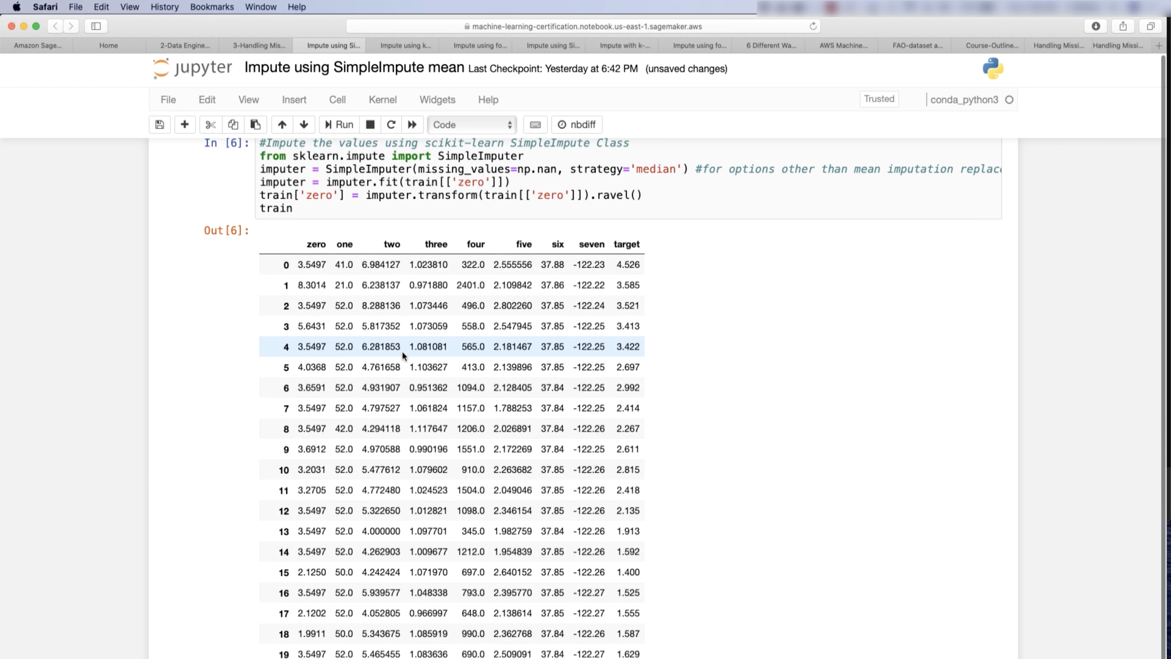
Impute missing values for continuous variable
Impute missing values for categorical variable
Other Imputation Methods
Using Algorithms that support missing values
Prediction of missing values
Imputation using Deep Learning Library — Datawig

Do nothing
- Cause linear regression error
Remove the entire records
- Risk losing data points with valuable information
Mode/median/average value replacement
- Reflection of the other values in the feature
- Doesn’t factor correlation between features
- Can’t use on categorical feature
Most frequent value replacement
- Doesn’t factor correlation between features
- Works with categorical features
- Can introduce bias into your model
Model-based imputation
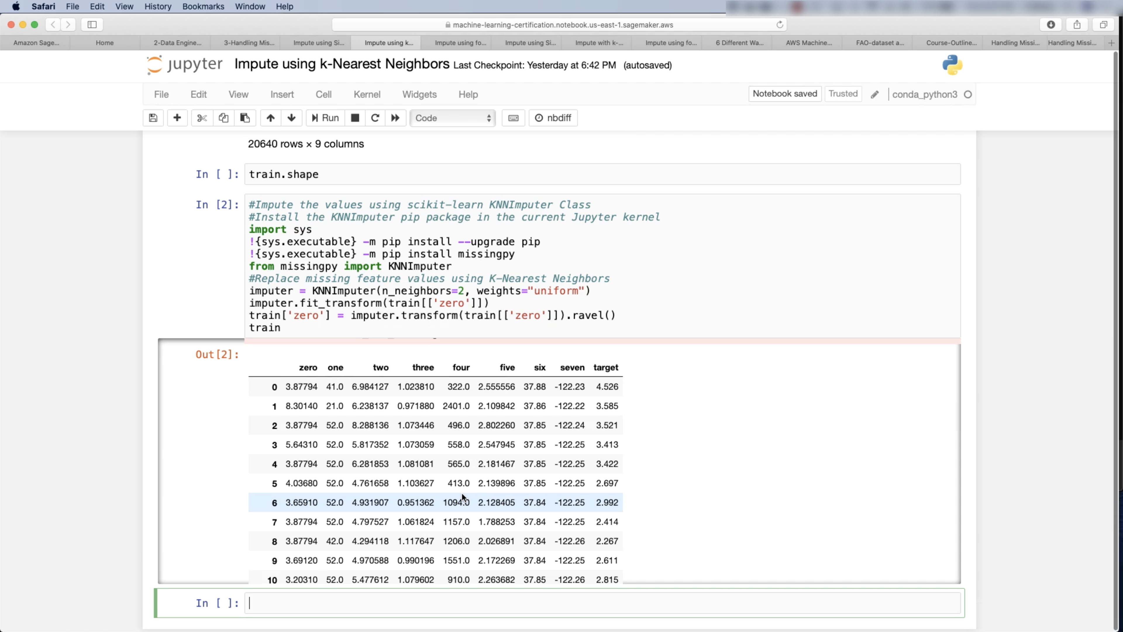
- KNN
  - Uses feature similarity to predict missing values
- Regression
  - Predictors of the variable with missing values identified via correlation matrix
  - Best predictors are selected and used as independent variables in a regression equation
  - Variable with missing data is used as the target variable
- Deep Learning
  - Works very well with categorical and non-numerical features
Other Methods
- Interpolation / Extrapolation
  - Estimate values from other observations within the range of a discrete set of known data points
- Forward filling / Backward filling
  - Fill the missing value by filling it from the preceding value or the succeeding value
- Hot deck imputation
  - Randomly choosing the missing value from a set of related and similar variables

Do nothing and let your algorithm either replace them through imputation (XGBoost) or just ignore them as LightGBM does with its use_missing = false parameter

A Comparison of Six Methods for Missing Data Imputation
In conclusion, bPCA(bayesian principal component analysis) and FKM(fuzzy K-means) are two imputation methods of interest. They outperform more popular approaches such as Mean, KNN, SVD(singular value decomposition) or MICE(multiple imputations by chained equations), and hence deserve further consideration in practice.

Handling Missing Values when Applying Classification Models
What Do We Do with Missing Data? Some Options for Analysis of Incomplete Data
Feature Processing

Drop Missing Data

Python

df.dropna(inplace=True) # Drop any row with a missing value
df_notna = df.dropna(axis=0) # Drop any row with a missing value

df.dropna(axis=0, how='all') # Drop only rows with all missing values 

df.dropna(subset=['<col_name>'], how='any') # Drop only rows with missing values in the specific column

Python

d = pd.DataFrame({'a': [np.nan, np.nan], 'b': [np.nan, 0]})
d

d.isna().all(axis=0)

d.isna().all(axis=1)

d.dropna(how='all', axis=0)

d.dropna(how='all', axis=1)

Imputation: mean, mode

Python

from sklearn.model_selection import train_test_split
from sklearn.impute import SimpleImputer

X_train, X_test, y_train, y_test = train_test_split(X, y, test_size=0.3, random_state=1)

# Fill in the lines below: imputation
imp_mean = SimpleImputer(missing_values=np.nan, strategy='mean')
imputed_X_train = pd.DataFrame(imp_mean.fit_transform(X_train))
imputed_X_valid = pd.DataFrame(imp_mean.transform(X_test))

# Fill in the lines below: imputation removed column names; put them back
imputed_X_train.columns = X_train.columns
imputed_X_valid.columns = X_test.columns

Outliers

A Brief Overview of Outlier Detection Techniques
A Density-based algorithm for outlier detection

Types of Outliers

In general, outliers can be classified into three categories, namely global outliers, contextual (or conditional) outliers, and collective outliers.

Global outlier — Object significantly deviates from the rest of the data set
Contextual outlier — Object deviates significantly based on a selected context. For example, 28⁰C is an outlier for a Moscow winter, but not an outlier in another context, 28⁰C is not an outlier for a Moscow summer.
Collective outlier — A subset of data objects collectively deviate significantly from the whole data set, even if the individual data objects may not be outliers. For example, a large set of transactions of the same stock among a small party in a short period can be considered as an evidence of market manipulation.

Outliers Detection

Also, when starting an outlier detection quest you have to answer two important questions about your dataset:

Which and how many features am I taking into account to detect outliers ? (univariate / multivariate)
Can I assume a distribution(s) of values for my selected features? (parametric / non-parametric)

Some of the most popular methods for outlier detection are:

Z-Score or Extreme Value Analysis (parametric)
Probabilistic and Statistical Modeling (parametric)
Linear Regression Models (PCA, LMS)
Proximity Based Models (non-parametric)
- Dbscan (Density Based Spatial Clustering of Applications with Noise, non-parametric)
Information Theory Models
High Dimensional Outlier Detection Methods (high dimensional sparse data)
Isolation Forests (non-parametric)

Z-Score pros:

It is a very effective method if you can describe the values in the feature space with a gaussian distribution. (Parametric)
The implementation is very easy using pandas and scipy.stats libraries.

Z-Score cons:

It is only convenient to use in a low dimensional feature space, in a small to medium sized dataset.
Is not recommended when distributions can not be assumed to be parametric.

Dbscan pros:

It is a super effective method when the distribution of values in the feature space can not be assumed.
Works well if the feature space for searching outliers is multidimensional (ie. 3 or more dimensions)
Sci-kit learn’s implementation is easy to use and the documentation is superb.
Visualizing the results is easy and the method itself is very intuitive.

Dbscan cons:

The values in the feature space need to be scaled accordingly.
Selecting the optimal parameters eps, MinPts and metric can be difficult since it is very sensitive to any of the three params.
It is an unsupervised model and needs to be re-calibrated each time a new batch of data is analyzed.
It can predict once calibrated but is strongly not recommended.

Isolation Forest pros:

There is no need of scaling the values in the feature space.
It is an effective method when value distributions can not be assumed.
It has few parameters, this makes this method fairly robust and easy to optimize.
Scikit-Learn’s implementation is easy to use and the documentation is superb.

Isolation Forest cons:

The Python implementation exists only in the development version of Sklearn.
Visualizing results is complicated.
If not correctly optimized, training time can be very long and computationally expensive.

Dbscan

[sklearn.preprocessing.RobustScaler](https://scikit-learn.org/stable/modules/generated/sklearn.preprocessing.RobustScaler.html

Isolation Forests

Encoding

What is One-Hot Encoding and how to use Pandas get_dummies function
Dummy variable (statistics)
ML | Dummy variable trap in Regression Models

Kaggle Intermediate Machine Learning: Categorical Variables

Integer Encoding: encodes the values as integer.
One-Hot Encoding: encodes the values as a binary vector array.
Dummy Variable Encoding: same as One-Hot Encoding, but one less column.

One-hot Encoding

Python

1
2
3

pd.get_dummies(df[col], drop_first=False) # one-hot encoding, fill NaN with 0

pd.get_dummies(df[col], drop_first=False, dummy_na=True) # one-hot encoding, including NaN column

Dummy Variable Encoding

Python

1
2
3

pd.get_dummies(df[col], drop_first=True) # dummy variables encoding, fill NaN with 0

pd.get_dummies(df[col], drop_first=True, dummy_na=True) # dummy variables encoding, including NaN column

Dummy encoding variable is a standard advice in statistics to avoid the dummy variable trap, However, in the world of machine learning, One-Hot encoding is more recommended because dummy variable trap is not really a problem when applying regularization.

Dummy Variable Trap:
The Dummy variable trap is a scenario where there are attributes which are highly correlated (Multicollinear) and one variable predicts the value of others. When we use one hot encoding for handling the categorical data, then one dummy variable (attribute) can be predicted with the help of other dummy variables. Hence, one dummy variable is highly correlated with other dummy variables. Using all dummy variables for regression models lead to dummy variable trap. So, the regression models should be designed excluding one dummy variable.

For Example –
Let’s consider the case of gender having two values male (0 or 1) and female (1 or 0). Including both the dummy variable can cause redundancy because if a person is not male in such case that person is a female, hence, we don’t need to use both the variables in regression models. This will protect us from dummy variable trap.

Ordinal Encoding

Kaggle Intermediate Machine Learning: Categorical Variables

Preprocessing

Pipeline

Pipelines

Step 1: Define Preprocessing Steps
Similar to how a pipeline bundles together preprocessing and modeling steps, we use the ColumnTransformer class to bundle together different preprocessing steps. The code below:

imputes missing values in numerical data, and
imputes missing values and applies a one-hot encoding to categorical data.

Python

from sklearn.compose import ColumnTransformer
from sklearn.pipeline import Pipeline
from sklearn.impute import SimpleImputer
from sklearn.preprocessing import OneHotEncoder

# Preprocessing for numerical data
numerical_transformer = SimpleImputer(strategy='constant')

# Preprocessing for categorical data
categorical_transformer = Pipeline(steps=[
    ('imputer', SimpleImputer(strategy='most_frequent')),
    ('onehot', OneHotEncoder(handle_unknown='ignore'))
])

# Bundle preprocessing for numerical and categorical data
preprocessor = ColumnTransformer(
    transformers=[
        ('num', numerical_transformer, numerical_cols),
        ('cat', categorical_transformer, categorical_cols)
    ])

Step 2: Define the Model
Next, we define a random forest model with the familiar RandomForestRegressor class.

Python

1
2
3

from sklearn.ensemble import RandomForestRegressor

model = RandomForestRegressor(n_estimators=100, random_state=0)

Step 3: Create and Evaluate the Pipeline
Finally, we use the Pipeline class to define a pipeline that bundles the preprocessing and modeling steps. There are a few important things to notice:

With the pipeline, we preprocess the training data and fit the model in a single line of code. (In contrast, without a pipeline, we have to do imputation, one-hot encoding, and model training in separate steps. This becomes especially messy if we have to deal with both numerical and categorical variables!)
With the pipeline, we supply the unprocessed features in X_valid to the predict() command, and the pipeline automatically preprocesses the features before generating predictions. (However, without a pipeline, we have to remember to preprocess the validation data before making predictions.)

Python

from sklearn.metrics import mean_absolute_error

# Bundle preprocessing and modeling code in a pipeline
my_pipeline = Pipeline(steps=[('preprocessor', preprocessor),
                              ('model', model)
                             ])

# Preprocessing of training data, fit model 
my_pipeline.fit(X_train, y_train)

# Preprocessing of validation data, get predictions
preds = my_pipeline.predict(X_valid)

# Evaluate the model
score = mean_absolute_error(y_valid, preds)
print('MAE:', score)

Count

Python

1 2	df.groupby(<col_name>)[<col_name>].count().sort_values(ascending=False) # count a column df.<col_name>.values_count(ascending=False) # count a column

Feature Engineering

An Introduction to Variable and Feature Selection

The purposes of feature selection:

Reduce the number features (e.g. gene selection & text categorization)

Usually fewer than 100 patients are available altogether for training and testing. But, the number of variables in the raw data range from 6,000 to 60,000.
In the text classification problem, the “bag-of-words” may reduce the effective number of words to 15,000. Large docuemnt collections of 5,000 to 800,000 documents are available for research.

Benefits:

Facilitating data visualization and data understanding
Reducing the measurement and storage requirements
Reducing training and utilization times
Defying the curse of dimensionality to improve prediction performance.

What is Feature Engineering

The Goal of Feature Engineering
The goal of feature engineering is simply to make your data better suited to the problem at hand.

Consider “apparent temperature” measures like the heat index and the wind chill. These quantities attempt to measure the perceived temperature to humans based on air temperature, humidity, and wind speed, things which we can measure directly. You could think of an apparent temperature as the result of a kind of feature engineering, an attempt to make the observed data more relevant to what we actually care about: how it actually feels outside!

You might perform feature engineering to:

improve a model’s predictive performance
reduce computational or data needs
improve interpretability of the results

Example

Example - Concrete Formulations

We’ll first establish a baseline by training the model on the un-augmented dataset. This will help us determine whether our new features are actually useful.

Establishing baselines like this is good practice at the start of the feature engineering process. A baseline score can help you decide whether your new features are worth keeping, or whether you should discard them and possibly try something else.

Mutual Information

First encountering a new dataset can sometimes feel overwhelming. You might be presented with hundreds or thousands of features without even a description to go by. Where do you even begin?

A great first step is to construct a ranking with a feature utility metric, a function measuring associations between a feature and the target. Then you can choose a smaller set of the most useful features to develop initially and have more confidence that your time will be well spent.

The metric we’ll use is called “mutual information”. Mutual information is a lot like correlation in that it measures a relationship between two quantities. The advantage of mutual information is that it can detect any kind of relationship, while correlation only detects linear relationships.

Mutual information is a great general-purpose metric and especially useful at the start of feature development when you might not know what model you’d like to use yet. It is:

easy to use and interpret,
computationally efficient,
theoretically well-founded,
resistant to overfitting, and,
able to detect any kind of relationship

Mutual Information and What it Measures

Mutual information describes relationships in terms of uncertainty. The mutual information (MI) between two quantities is a measure of the extent to which knowledge of one quantity reduces uncertainty about the other. If you knew the value of a feature, how much more confident would you be about the target?

Here’s an example from the Ames Housing data. The figure shows the relationship between the exterior quality of a house and the price it sold for. Each point represents a house.

Knowing the exterior quality of a house reduces uncertainty about its sale price.

From the figure, we can see that knowing the value of ExterQual should make you more certain about the corresponding SalePrice – each category of ExterQual tends to concentrate SalePrice to within a certain range. The mutual information that ExterQual has with SalePrice is the average reduction of uncertainty in SalePrice taken over the four values of ExterQual. Since Fair occurs less often than Typical, for instance, Fair gets less weight in the MI score.

(Technical note: What we’re calling uncertainty is measured using a quantity from information theory known as “entropy”. The entropy of a variable means roughly: “how many yes-or-no questions you would need to describe an occurance of that variable, on average.” The more questions you have to ask, the more uncertain you must be about the variable. Mutual information is how many questions you expect the feature to answer about the target.)

Interpreting Mutual Information Scores

The least possible mutual information between quantities is 0.0. When MI is zero, the quantities are independent: neither can tell you anything about the other. Conversely, in theory there’s no upper bound to what MI can be. In practice though values above 2.0 or so are uncommon. (Mutual information is a logarithmic quantity, so it increases very slowly.)

The next figure will give you an idea of how MI values correspond to the kind and degree of association a feature has with the target.

Left: Mutual information increases as the dependence between feature and target becomes tighter.
Right: Mutual information can capture any kind of association (not just linear, like correlation.)

Here are some things to remember when applying mutual information:

MI can help you to understand the relative potential of a feature as a predictor of the target, considered by itself.
It’s possible for a feature to be very informative when interacting with other features, but not so informative all alone. MI can’t detect interactions between features. It is a univariate metric.
The actual usefulness of a feature depends on the model you use it with. A feature is only useful to the extent that its relationship with the target is one your model can learn. Just because a feature has a high MI score doesn’t mean your model will be able to do anything with that information. You may need to transform the feature first to expose the association.

Example - 1985 Automobiles

automobile-mutual-information.ipynb

Creating Features

creating-features

Tips on Discovering New Features

Understand the features. Refer to your dataset’s data documentation, if available.
Research the problem domain to acquire domain knowledge. If your problem is predicting house prices, do some research on real-estate for instance. Wikipedia can be a good starting point, but books and journal articles will often have the best information.
Study previous work. Solution write-ups from past Kaggle competitions are a great resource.
Use data visualization. Visualization can reveal pathologies in the distribution of a feature or complicated relationships that could be simplified. Be sure to visualize your dataset as you work through the feature engineering process.

Tips on Creating Features
It’s good to keep in mind your model’s own strengths and weaknesses when creating features. Here are some guidelines:

Linear models learn sums and differences naturally, but can’t learn anything more complex.
Ratios seem to be difficult for most models to learn. Ratio combinations often lead to some easy performance gains.
Linear models and neural nets generally do better with normalized features. Neural nets especially need features scaled to - values not too far from 0. Tree-based models (like random forests and XGBoost) can sometimes benefit from normalization, but usually much less so.
Tree models can learn to approximate almost any combination of features, but when a combination is especially important they can still benefit from having it explicitly created, especially when data is limited.
Counts are especially helpful for tree models, since these models don’t have a natural way of aggregating information across many features at once.

Clustering with K-mean

clustering-with-k-means.ipynb
exercise-clustering-with-k-means.ipynb

Principal Component Analysis

StatQuest: Principal Component Analysis (PCA), Step-by-Step
Data Analysis 6: Principal Component Analysis (PCA) - Computerphile
principal-component-analysis.ipynb
exercise-principal-component-analysis.ipynb

PCA for Feature Engineering

There are two ways you could use PCA for feature engineering.

The first way is to use it as a descriptive technique. Since the components tell you about the variation, you could compute the MI scores for the components and see what kind of variation is most predictive of your target.

The second way is to use the components themselves as features. Because the components expose the variational structure of the data directly, they can often be more informative than the original features. Here are some use-cases:

Dimensionality reduction: When your features are highly redundant (multicollinear, specifically), PCA will partition out the redundancy into one or more near-zero variance components, which you can then drop since they will contain little or no information.
Anomaly detection: Unusual variation, not apparent from the original features, will often show up in the low-variance components. These components could be highly informative in an anomaly or outlier detection task.
Noise reduction: A collection of sensor readings will often share some common background noise. PCA can sometimes collect the (informative) signal into a smaller number of features while leaving the noise alone, thus boosting the signal-to-noise ratio.
Decorrelation: Some ML algorithms struggle with highly-correlated features. PCA transforms correlated features into uncorrelated components, which could be easier for your algorithm to work with.
PCA basically gives you direct access to the correlational structure of your data. You’ll no doubt come up with applications of your own!

PCA Best Practices

There are a few things to keep in mind when applying PCA:

PCA only works with numeric features, like continuous quantities or counts.
PCA is sensitive to scale. It’s good practice to standardize your data before applying PCA, unless you know you have good reason not to.
Consider removing or constraining outliers, since they can an have an undue influence on the results.

Target Encoding

target-encoding.ipynb
exercise-target-encoding.ipynb

Modeling

Supervised Learning

Decision Tree

Decision Tree: Regression Tree and Classification Tree

Pro:

Simple to understand, interpret, visualize
Work for either classification or regression task.
Little effort for data preparation.
Nonlinear relationships between parameters do not affect the clip performance

Cons:

Overfitting
Decision Trees can be unstable because small variations(variance) in the data.
Greedy algorithms cannot guarantee to return the globally optimal Decision Tree. This can be mitigated by training multiple trees.
Decision Tree learners also create bias tree if some classes dominate it is therefore recommended to balance dataset priority setting what the decision tree.

What is Greedy algorithms?
A greedy algorithm, as the name suggests, always makes the choice that seems to be the best at that moment. This means that it makes locally-optimal choice in the hope that this choice will lead to a globally-optimal solution.

PRUNING

Random Forest

Random Forest

Decision Trees vote.

Pros:

Powerful
Work for either classification or regression task.
Handle the missing values and maintains accuracy for missing data.
Won’t overfit the model.
Handle large dataset with higher dimensionality.

Cons:

Good job at classification but not as good as for regression.
You have very little control on what the model does.

Usage:

Identifying loyal users or fraud users.
Analyzing the patients’ medical records.
Identifying stock behaviors.
Recommender System (small segment of the recommendation engine).
Computer Vision for image classification.
Voice classification.

XGBoost

XGBoost

Introduction

For much of this course, you have made predictions with the random forest method, which achieves better performance than a single decision tree simply by averaging the predictions of many decision trees.

We refer to the random forest method as an “ensemble method“. By definition, ensemble methods combine the predictions of several models (e.g., several trees, in the case of random forests).

Next, we’ll learn about another ensemble method called gradient boosting.

Gradient Boosting

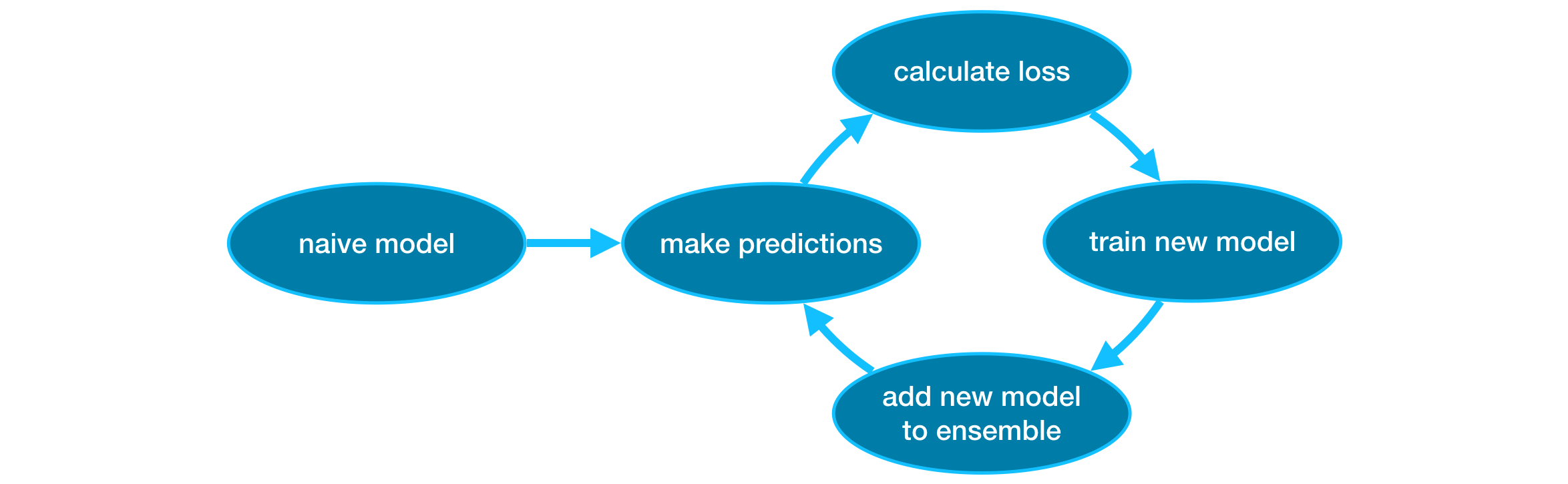
Gradient boosting is a method that goes through cycles to iteratively add models into an ensemble.

It begins by initializing the ensemble with a single model, whose predictions can be pretty naive. (Even if its predictions are wildly inaccurate, subsequent additions to the ensemble will address those errors.)

Then, we start the cycle:

First, we use the current ensemble to generate predictions for each observation in the dataset. To make a prediction, we add the predictions from all models in the ensemble.
These predictions are used to calculate a loss function (like mean squared error, for instance).
Then, we use the loss function to fit a new model that will be added to the ensemble. Specifically, we determine model parameters so that adding this new model to the ensemble will reduce the loss. (Side note: The “gradient” in “gradient boosting” refers to the fact that we’ll use gradient descent on the loss function to determine the parameters in this new model.)
Finally, we add the new model to ensemble, and …
… repeat!

Parameter Tuning

XGBoost has a few parameters that can dramatically affect accuracy and training speed. The first parameters you should understand are:

n_estimators
n_estimators specifies how many times to go through the modeling cycle described above. It is equal to the number of models that we include in the ensemble.

Too low a value causes underfitting, which leads to inaccurate predictions on both training data and test data.
Too high a value causes overfitting, which causes accurate predictions on training data, but inaccurate predictions on test data (which is what we care about).

Typical values range from 100-1000, though this depends a lot on the learning_rate parameter discussed below.

Here is the code to set the number of models in the ensemble:

Python

1 2	my_model = XGBRegressor(n_estimators=500) my_model.fit(X_train, y_train)

early_stopping_rounds
early_stopping_rounds offers a way to automatically find the ideal value for n_estimators. Early stopping causes the model to stop iterating when the validation score stops improving, even if we aren’t at the hard stop for n_estimators. It’s smart to set a high value for n_estimators and then use early_stopping_rounds to find the optimal time to stop iterating.

Since random chance sometimes causes a single round where validation scores don’t improve, you need to specify a number for how many rounds of straight deterioration to allow before stopping. Setting early_stopping_rounds=5 is a reasonable choice. In this case, we stop after 5 straight rounds of deteriorating validation scores.

When using early_stopping_rounds, you also need to set aside some data for calculating the validation scores - this is done by setting the eval_set parameter.

We can modify the example above to include early stopping:

Python

my_model = XGBRegressor(n_estimators=500)
my_model.fit(X_train, y_train, 
             early_stopping_rounds=5, 
             eval_set=[(X_valid, y_valid)],
             verbose=False)

If you later want to fit a model with all of your data, set n_estimators to whatever value you found to be optimal when run with early stopping.

learning_rate
Instead of getting predictions by simply adding up the predictions from each component model, we can multiply the predictions from each model by a small number (known as the learning rate) before adding them in.

This means each tree we add to the ensemble helps us less. So, we can set a higher value for n_estimators without overfitting. If we use early stopping, the appropriate number of trees will be determined automatically.

In general, a small learning rate and large number of estimators will yield more accurate XGBoost models, though it will also take the model longer to train since it does more iterations through the cycle. As default, XGBoost sets learning_rate=0.1.

Modifying the example above to change the learning rate yields the following code:

Python

my_model = XGBRegressor(n_estimators=1000, learning_rate=0.05)
my_model.fit(X_train, y_train, 
             early_stopping_rounds=5, 
             eval_set=[(X_valid, y_valid)], 
             verbose=False)

n_jobs
On larger datasets where runtime is a consideration, you can use parallelism to build your models faster. It’s common to set the parameter n_jobs equal to the number of cores on your machine. On smaller datasets, this won’t help.

The resulting model won’t be any better, so micro-optimizing for fitting time is typically nothing but a distraction. But, it’s useful in large datasets where you would otherwise spend a long time waiting during the fit command.

Here’s the modified example:

Python

my_model = XGBRegressor(n_estimators=1000, learning_rate=0.05, n_jobs=4)
my_model.fit(X_train, y_train, 
             early_stopping_rounds=5, 
             eval_set=[(X_valid, y_valid)], 
             verbose=False)

Conclusion

XGBoost is a the leading software library for working with standard tabular data (the type of data you store in Pandas DataFrames, as opposed to more exotic types of data like images and videos). With careful parameter tuning, you can train highly accurate models.

Cross-Validation

What is cross-validation?

In cross-validation, we run our modeling process on different subsets of the data to get multiple measures of model quality.

For example, we could begin by dividing the data into 5 pieces, each 20% of the full dataset. In this case, we say that we have broken the data into 5 “folds”.

When should you use cross-validation?

Cross-validation gives a more accurate measure of model quality, which is especially important if you are making a lot of modeling decisions. However, it can take longer to run, because it estimates multiple models (one for each fold).

So, given these tradeoffs, when should you use each approach?

For small datasets, where extra computational burden isn’t a big deal, you should run cross-validation.
For larger datasets, a single validation set is sufficient. Your code will run faster, and you may have enough data that there’s little need to re-use some of it for holdout.

There’s no simple threshold for what constitutes a large vs. small dataset. But if your model takes a couple minutes or less to run, it’s probably worth switching to cross-validation.

Alternatively, you can run cross-validation and see if the scores for each experiment seem close. If each experiment yields the same results, a single validation set is probably sufficient.

Metrics and scoring: quantifying the quality of predictions

Data Leakage

Data Leakage

Target leakage
Target leakage occurs when your predictors include data that will not be available at the time you make predictions. It is important to think about target leakage in terms of the timing or chronological order that data becomes available, not merely whether a feature helps make good predictions.

Train-Test Contamination
A different type of leak occurs when you aren’t careful to distinguish training data from validation data.

Recall that validation is meant to be a measure of how the model does on data that it hasn’t considered before. You can corrupt this process in subtle ways if the validation data affects the preprocessing behavior. This is sometimes called train-test contamination.

Data Science

Data8

Udacity Data Scientist

Enterprise Analytics

Probability Theory and Introductory Statistics

Hypothesis Testing

Formulas

Statistics

Expected value

Expected value

Finite case

$\displaystyle E[X] = \sum_{i=1}^{k}{x_i p_i}$

Countably Infinite case

$\displaystyle E[X] = \sum_{i=1}^{\infty}{x_i p_i}$

Expected values of common distributions

Distribution	Notation	Mean E(X)
Bernoulli	$X\sim ~b(1,p)$	$p$
Binomial	$X\sim B(n,p)$	$np$
Poisson	$X\sim Po(\lambda )$	$\lambda$
Geometric	$X\sim Geometric(p)$	$1/p$
Uniform	$X\sim U(a,b)$	$(a+b)/2$
Exponential	$X\sim \exp(\lambda )$	$1/\lambda$
Normal	$X\sim N(\mu ,\sigma ^{2})$	$\mu$
Standard Normal	$X\sim N(0,1)$
Pareto	$X\sim Par(\alpha )$	$\alpha /(\alpha +1)$ if $\alpha >1$
Cauchy	$X\sim Cauchy(x_{0},\gamma )$	undefined

Standard Deviation

Standard deviation

$\displaystyle \sigma^2 \equiv E[X] = \frac{1}{N} \sum_{i=1}^{N}{(x_i - \mu)^2}$

$\displaystyle \sigma \equiv \sqrt{E[(X - \mu)^2]} = \sqrt{\frac{1}{N} \sum_{i=1}^{N}{(x_i - \mu)^2}}$

Covariance

Covariance

$\displaystyle cov(X, Y) = E[(X - E[X])(Y - E[Y])] = \frac{\sum{(x_i - \bar x)(y_i - \bar y)}}{N}$

Pearson correlation coefficient

Pearson correlation coefficient

$\displaystyle \rho_{X, Y} = \frac{cov(X, Y)}{\sigma_X \sigma_Y}$

where:

$cov$ is the covariance
$\sigma_X$ is the standard deviation of $X$
$\sigma_Y$ is the standard deviation of $Y$

Import Dataset

CSV

JSON

XML

Database

SQLite3

sqlalchemy

sqlite

mysql

PostgreSQL

EDA

Database Info

DataFrame Info

Table dimensionality

Columns

Missing Data

Detect Missing Data

Handle Missing Data

Drop Missing Data

Imputation: mean, mode

Outliers

Types of Outliers

Outliers Detection

Dbscan

Isolation Forests

Encoding

Ordinal Encoding

Preprocessing

Pipeline

Count

Feature Engineering

What is Feature Engineering

Example

Mutual Information

Mutual Information and What it Measures

Interpreting Mutual Information Scores

Example - 1985 Automobiles

Creating Features

Clustering with K-mean

Principal Component Analysis

PCA for Feature Engineering

PCA Best Practices

Target Encoding

Modeling

Supervised Learning

Decision Tree

Random Forest

XGBoost

Introduction

Gradient Boosting

Parameter Tuning

Conclusion

Cross-Validation

What is cross-validation?

When should you use cross-validation?

Data Leakage

Related Posts

Data Science

Hypothesis Testing

A/B Testing

Artificial Intelligence

Supervised Learning

Formulas

Statistics

Expected value

Finite case

Countably Infinite case

Expected values of common distributions

Standard Deviation

Covariance

Pearson correlation coefficient

Regression