Enterprise Analytics
ALY6050
Reference
Statistics, Data Analysis, and Decision Modeling, Fifth Edition
James R. Evans
Copyright ©2013 Pearson Education, Inc. publishing as Prentice Hall
STATISTICAL SUPPORT
R
Excel
- Using statistical functions that are entered in worksheet cells directly or embedded in formulas.
- Using the Excel Analysis Toolpak add‐in to perform more complex statistical computations.
- Using the Prentice‐Hall statistics add‐in, PHStat, to perform analyses not designed into Excel.
Displaying data with Excel Charts
Column and Bar Charts
Excel distinguishes between vertical and horizontal bar charts, calling the former column charts and the latter bar charts. A clustered column chart compares values across categories using vertical rectangles; a stacked column chart displays the contribution of each value to the total by stacking the rectangles; and a 100% stacked column chart compares the percentage that each value contributes to a total.
Line Charts
Line charts provide a useful means for displaying data over time.
Pie Charts
For many types of data, we are interested in understanding the relative proportion of each data source to the total.
Area Charts
An area chart combines the features of a pie chart with those of line charts.
Scatter Diagrams
Scatter diagrams show the relationship between two variables.
Miscellaneous Excel Charts
Excel provides several additional charts for special applications. A stock chart allows you to plot stock prices, such as the daily high, low, and close. It may also be used for scientific data such as temperature changes. A surface chart shows three‐dimensional data. A doughnut chart is similar to a pie chart but can contain more than one data series. A bubble chart is a type of scatter chart in which the size of the data marker corresponds to the value of a third variable; consequently, it is a way to plot three variables in two dimensions. Finally, a radar chart allows you to plot multiple dimensions of several data series.
Ethics and Data Presentation
In summary, tables of numbers often hide more than they inform. Graphical displays clearly make it easier to gain insights about the data. Thus, graphs and charts are a means of converting raw data into useful managerial information. However, it can be easy to distort data by manipulating the scale on the chart. For example, Figure 1.23 shows the U.S. exports to China in Figure 1.17 displayed on a different scale. The pattern looks much flatter and suggests that the rate of exports is not increasing as fast as it really is. It is not unusual to see distorted graphs in newspapers and magazines that are intended to support the author’s conclusions. Creators of statistical displays have an ethical obligation to report data honestly and without attempts to distort the truth.
CHAPTER 2: DESCRIPTIVE STATISTICS AND DATA ANALYSIS
Introduction
Statistics:
- large population -> trough sample to summarize population
- predict large population <- measure sample
Data Types
When we deal with data, it is important to understand the type of data in order to select the appropriate statistical tool or procedure. One classification of data is the following:
- Types of data
• Cross‐sectional—data that are collected over a single period of time
• Time series—data collected over time - Number of variables
• Univariate—data consisting of a single variable
• Multivariate—data consisting of two or more (often related) variables
Example: Cross‐Sectional, Univariate Data
Descriptive Statistics
Quantitative measures and ways of describing data.
For example:
- measures of central tendency (mean, median, mode, proportion),
- measures of dispersion (range, variance, standard deviation), and
- frequency distributions and histograms.
Descriptive Statistics for Numerical Data
- Measures of location
- Measures of dispersion
- Measures of shape
- Measures of association
Measures of Location
Data Profiles (Fractiles)
Describe the location and spread of data over its range
- Quartiles – a division of a data set into four equal parts; shows the points below which 25%, 50%, 75% and 100% of the observations lie (25% is the first quartile, 75% is the third quartile, etc.)
- Deciles – a division of a data set into 10 equal parts; shows the points below which 10%, 20%, etc. of the observations lie
- Percentiles – a division of a data set into 100 equal parts; shows the points below which “k” percent of the observations lie
1 | ages <- c(5,31,43,48,50,41,7,11,15,39,80,82,32,2,8,6,25,36,27,61,31) |
1 | import numpy as np |
Measures of Central Tendency
Arithmetic Mean
- Population mean: $\mu = \displaystyle \frac{\sum^N_{i=1}x_i}{N}$
- Sample mean: $\bar x = \displaystyle \frac{\sum^N_{i=1}x_i}{n}$
- Excel function AVERAGE(data range)
1 | x <- c(0:10, 50) |
1 | import numpy as np |
Properties of the Mean
- Meaningful for interval and ratio data
- All data used in the calculation
- Unique for every set of data
- Affected by unusually large or small observations (outliers)
- The only measure of central tendency where the sum of the deviations of each value from the measure is zero; i.e., $\sum(x_i - \bar x) = 0$
Median
- Middle value when data are ordered from smallest to largest. This results in an equal number of observations above the median as below it.
- Unique for each set of data
- Not affected by extremes
- Meaningful for ratio, interval, and ordinal data
- Excel function MEDIAN(data range)
1 | x <- c(0:10) |
1 | import numpy as np |
Mode
- Observation that occurs most frequently; for grouped data, the midpoint of the cell with the largest frequency (approximate value)
- Useful when data consist of a small number of unique values
- Excel functions MODE.SNGL(data range) and MODE.MULT(data range)
1 | # Create the function. |
1 | from scipy import stats |
Midrange
- Average of the largest and smallest observations
- Useful for very small samples, but extreme values can distort the result
Measures of Dispersion
- Dispersion – the degree of variation in the data.
- Example:
- {48, 49, 50, 51, 52} vs. {10, 30, 50, 70, 90}
- Both means are 50, but the second data set has larger dispersion
- Example:
Range Measures
- Range – difference between the maximum and minimum observations
- Useful for very small samples, but extreme values can distort the result
- Interquartile range: $Q3 – Q1$
- Avoids problems with outliers
Variance
- Population variance: $\displaystyle \sigma^2 = \frac{\sum^N_{i=1}(x_i - \mu)^2}{N}$
- Sample variance: $\displaystyle s^2 = \frac{\sum^N_{i=1}(x_i - \bar x)^2}{n - 1}$
- Excel functions VAR.P(data range), VAR.S(data range)
1 | # Variance - Population |
1 | import numpy as np |
Standard Deviation
- Population SD: $\displaystyle \sigma = \sqrt{\frac{\sum^N_{i=1}(x_i - \mu)^2}{N}}$
- Sample SD: $\displaystyle s = \sqrt{\frac{\sum^N_{i=1}(x_i - \bar x)^2}{n - 1}}$
- The standard deviation has the same units of measurement as the original data, unlike the variance
- Excel functions STDEV.P(data range), STDEV.S(data range)
1 | # Standard Deviation - Population |
1 | import numpy as np |
Chebyshev’s Theorem
For any set of data, the proportion of values that lie within $k$ standard deviations of the mean is at least $1 – \frac{1}{k^2}$, for any $k > 1$
- For $k = 2$, at least 3⁄4 of the data lie within 2 standard deviations of the mean
- For $k = 3$, at least 8/9, or 89% lie within 3 standard deviations of the mean
- For $k = 10$, at least 99/100, or 99% of the data lie within 10 standard deviations of the mean
For example, if there are 36 students joining an exam with 80 as the average score and 10 as the standard deviation. Then the number of students less than 50 score will no more than 4($=36 \times \frac{1}{3^2}$).
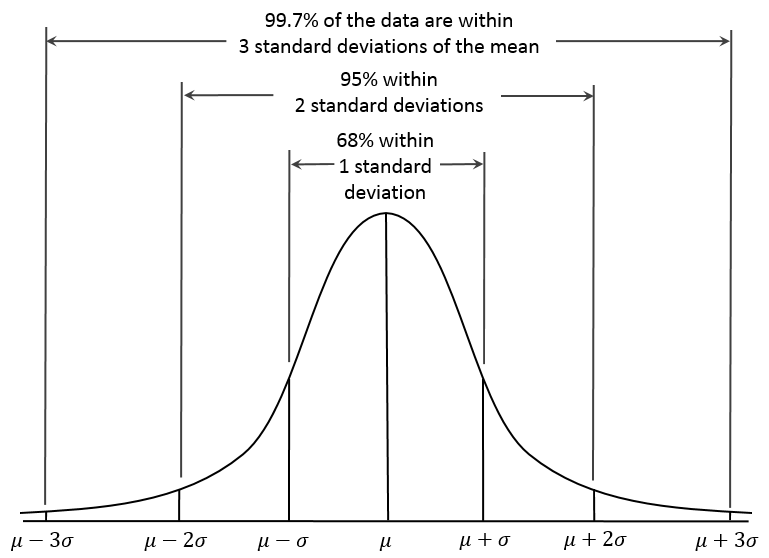
Empirical Rules
- Approximately 68% of the observations will fall within one standard deviation of the mean.
- Approximately 95% of the observations will fall within two standard deviations of the mean.
- Approximately 99.7% of the observations will fall within three standard deviations of the mean.
Coefficient of Variation
- CV = Standard Deviation / Mean $\displaystyle c_v = \frac{\sigma}{\mu}$
- CV is dimensionless, and therefore is useful when comparing data sets that are scaled differently.
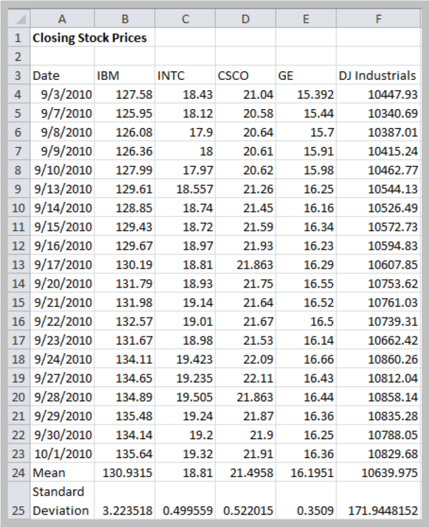
CV(IBM) = 0.025
CV(INTC) = 0.027
CV(CSCO) = 0.024
CV(GE) = 0.022
CV(DJI) = 0.016
Measures of Shape
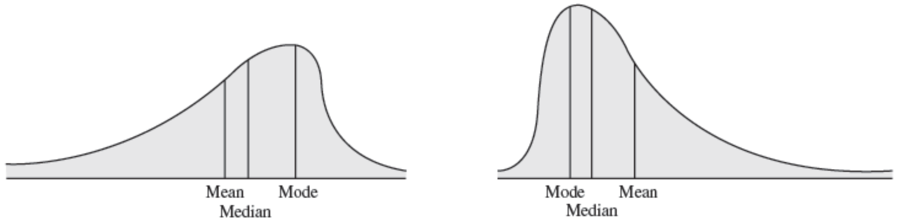
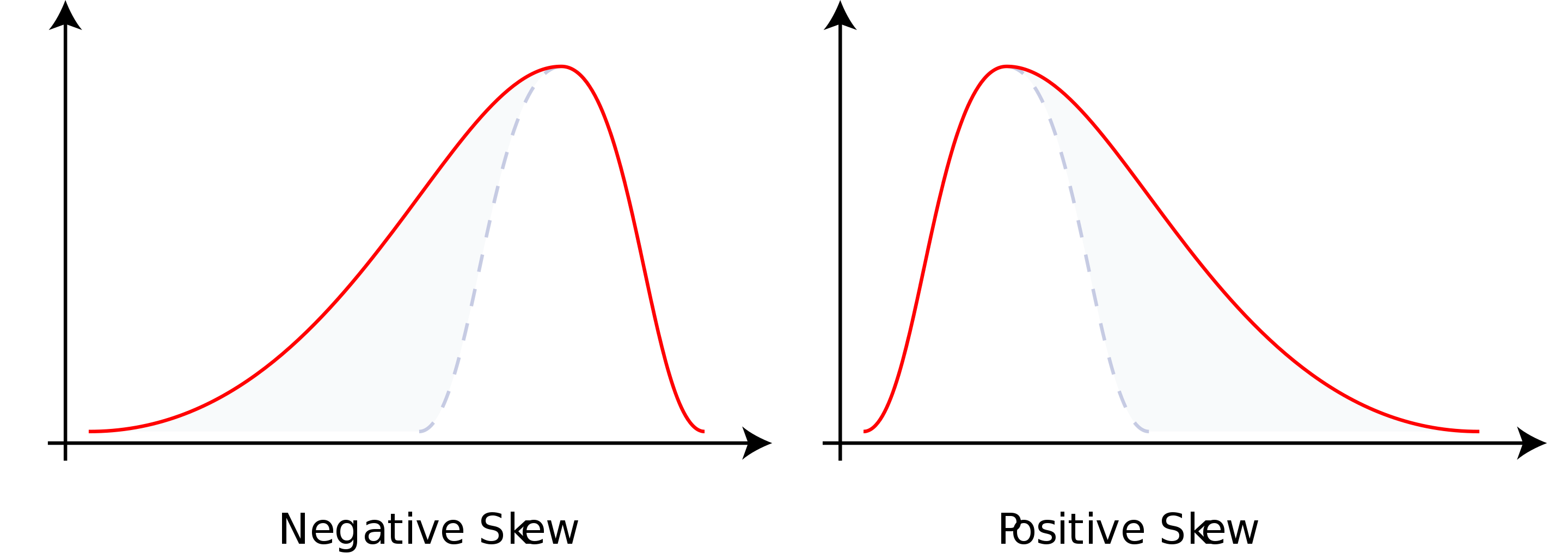
Skewness
- Coefficient of skewness (CS)
- $-0.5 < CS < 0.5$ indicates relative symmetry
- $CS > 1 \space or \space CS < -1$ indicates a high degree of skewness
- Mean - Median - Mode: Left Skewness(Negative Skewness)
- Mode - Median - Mean: Right Skewness(Positive Skewness)
- Excel function SKEW(data range)
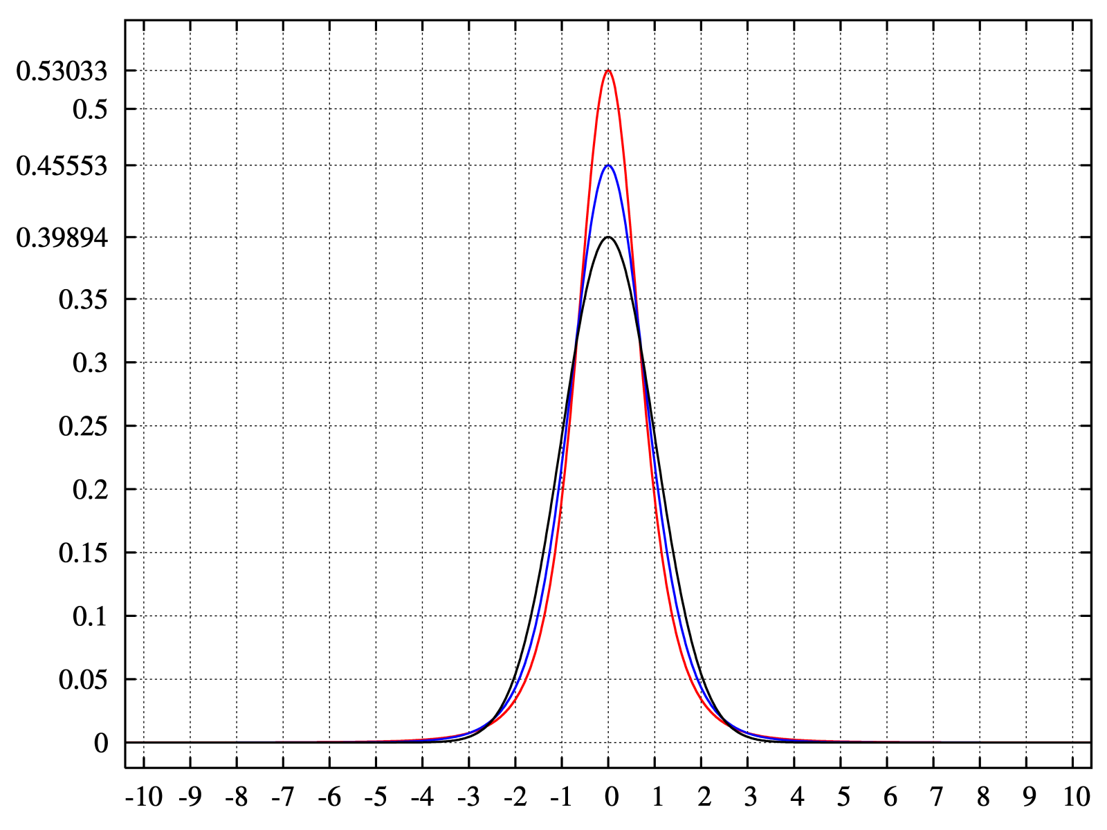
Kurtosis
- Refers to the peakedness or flatness of a distribution.
- Coefficient of kurtosis (CK)
- CK < 3: more flat with wide degree of dispersion
- CK > 3: more peaked with less dispersion
- The higher the kurtosis, the more area in the tails of the distribution
- Excel function KURT(data range)
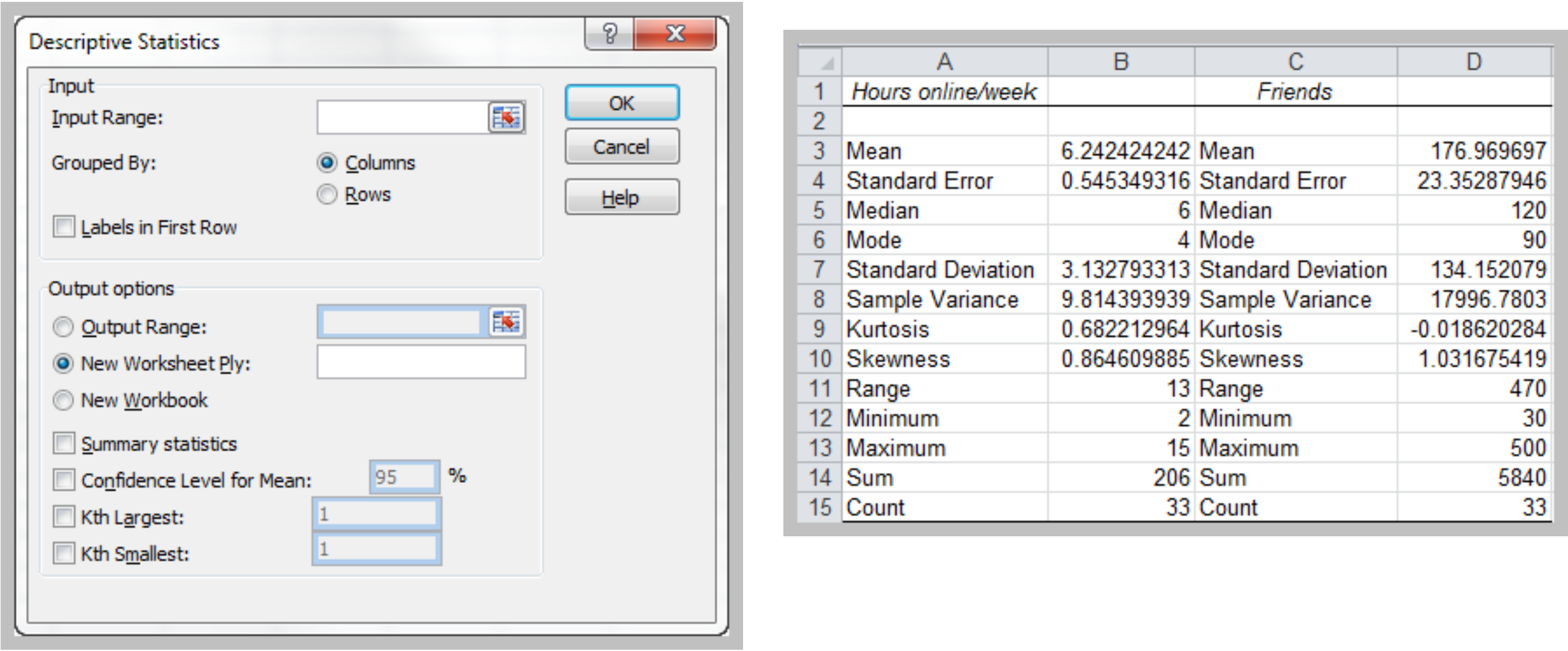
Excel Descriptive Statistics Tool
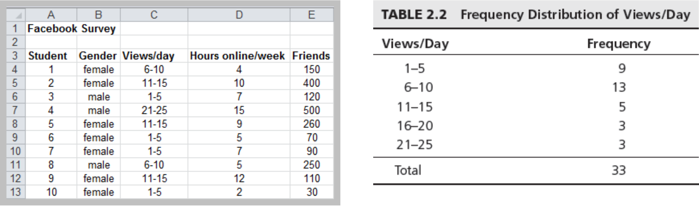
Frequency Distribution
- Tabular summary showing the frequency of observations in each of several non- overlapping classes, or cells
Excel Frequency Function
- Define bins
- Select a range of cells adjacent to the bin range (if continuous data, add one empty cell below this range as an overflow cell)
- Enter the formula =FREQUENCY(range of data, range of bins) and press Ctrl-Shift-Enter simultaneously.
- Construct a histogram using the Chart Wizard for a column chart.
Histogram
- A graphical representation of a frequency distribution
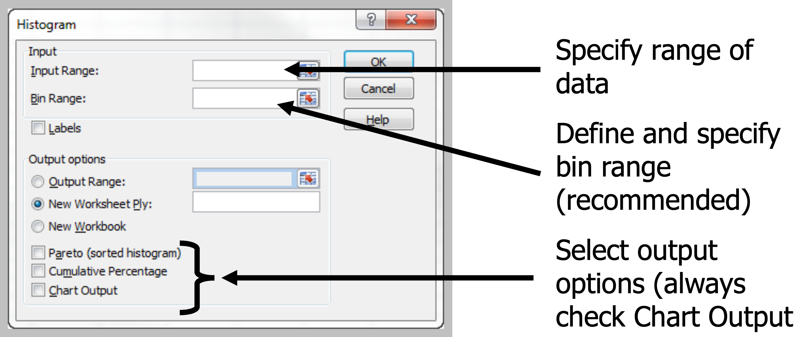
Excel Tool: Histogram
- Excel Menu > Tools > Data Analysis > Histogram
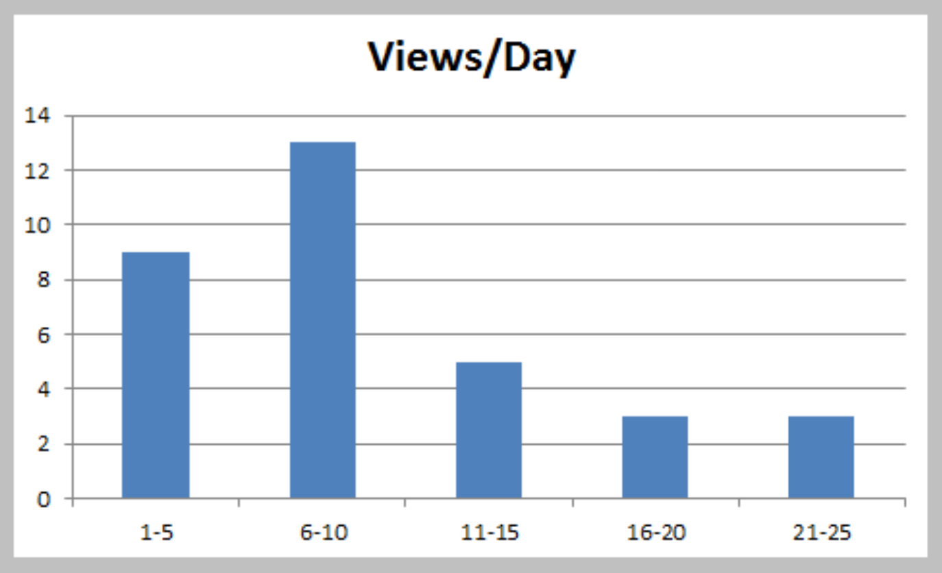
Histograms for Numerical Data – Few Discrete Values
- Leave Bin Range blank in Excel dialog.
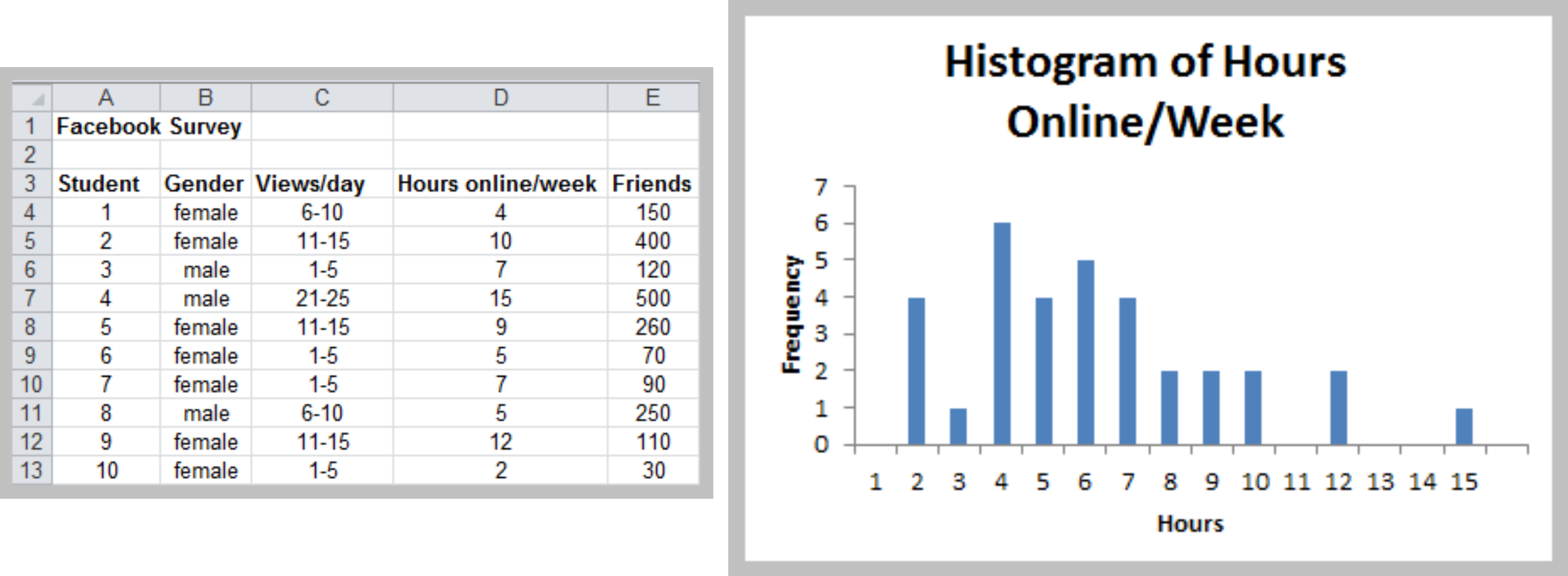
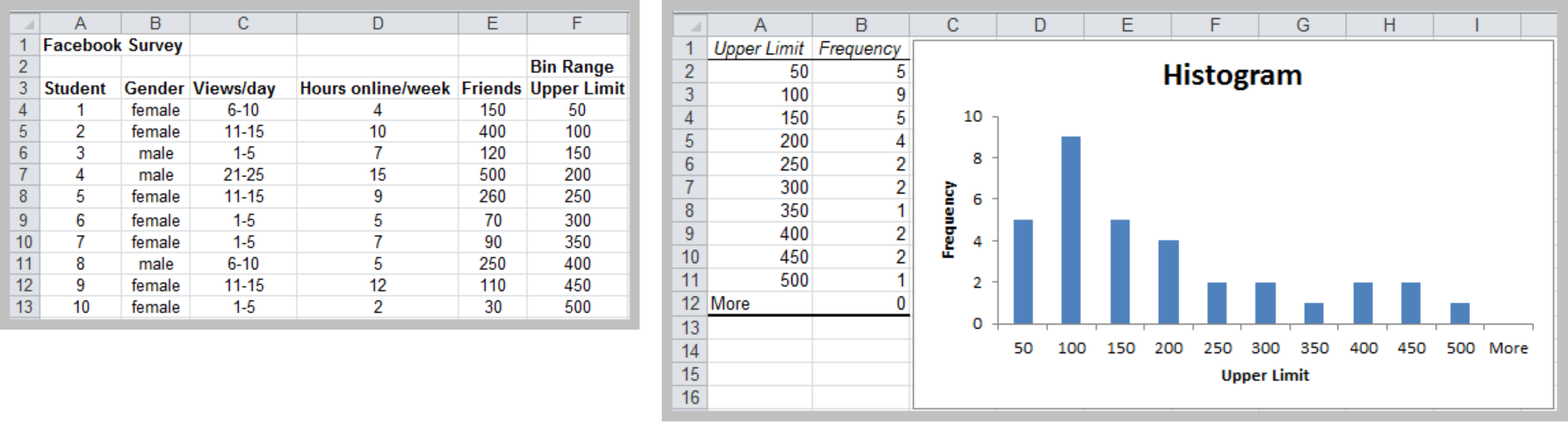
Histograms for Numerical Data – Many Discrete or Continuous Values
- Define a Bin Range in your spreadsheet
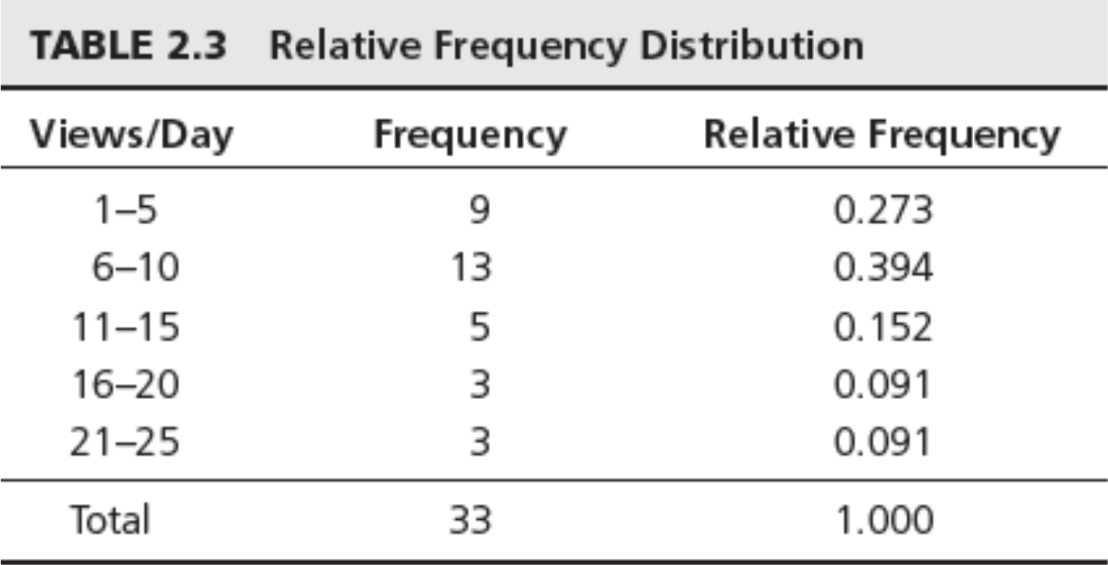
Relative Frequency Distribution
- Relative frequency – fraction or proportion of observations that fall within a cell
Cumulative Relative Frequency
- Cumulative relative frequency – proportion or percentage of observations that fall below the upper limit of a cell
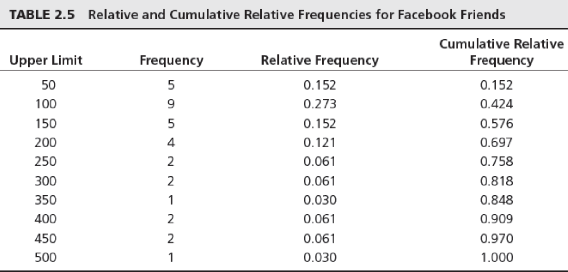
Chart of Cumulative Relative Frequency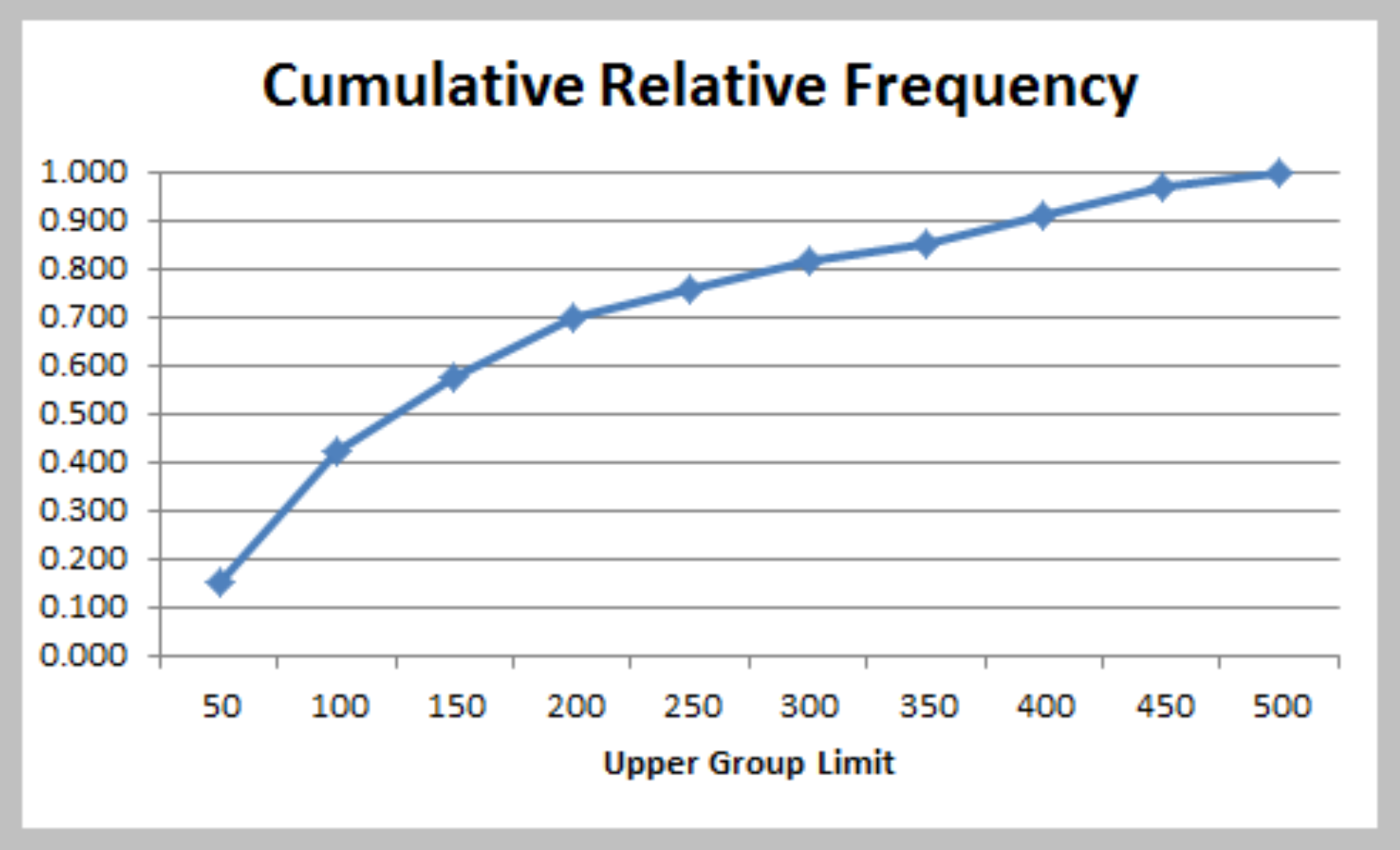
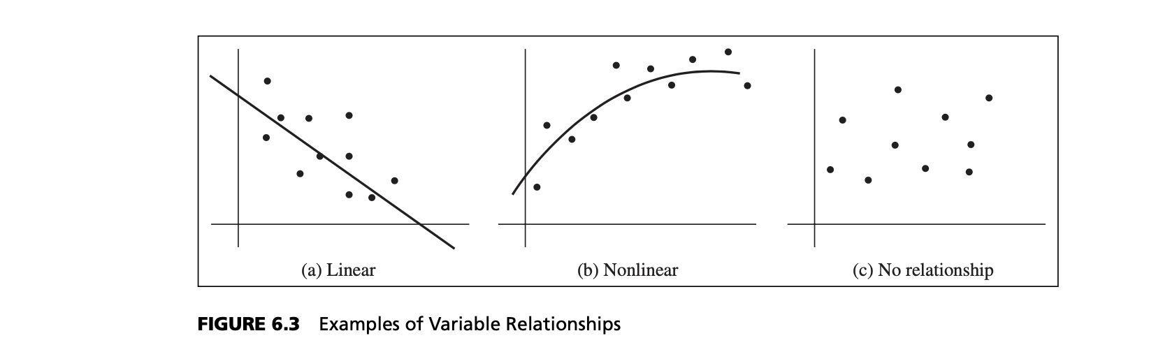
Measures of Association
- Correlation – a measure of strength of linear relationship between two variables
- Correlation coefficient – a number between -1 and 1.
- A correlation of 0 indicates that the two variables have no linear relationship to each other.
- A positive correlation coefficient indicates a linear relationship for which one variable increases as the other also increases.
- A negative correlation coefficient indicates a linear relationship for one variable that increases while the other decreases.
- Excel function CORREL or Data Analysis Correlation
tool
Examples of Correlation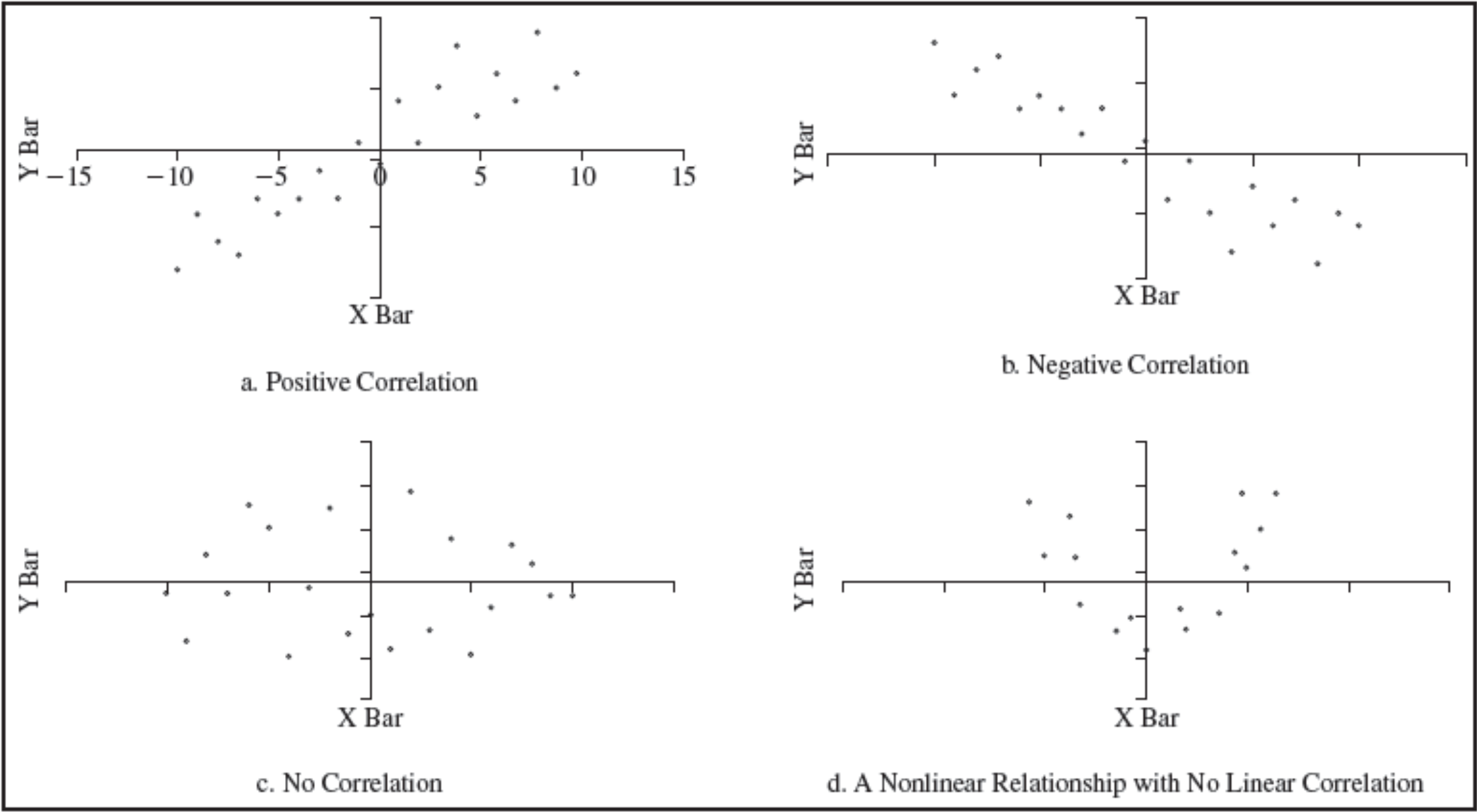
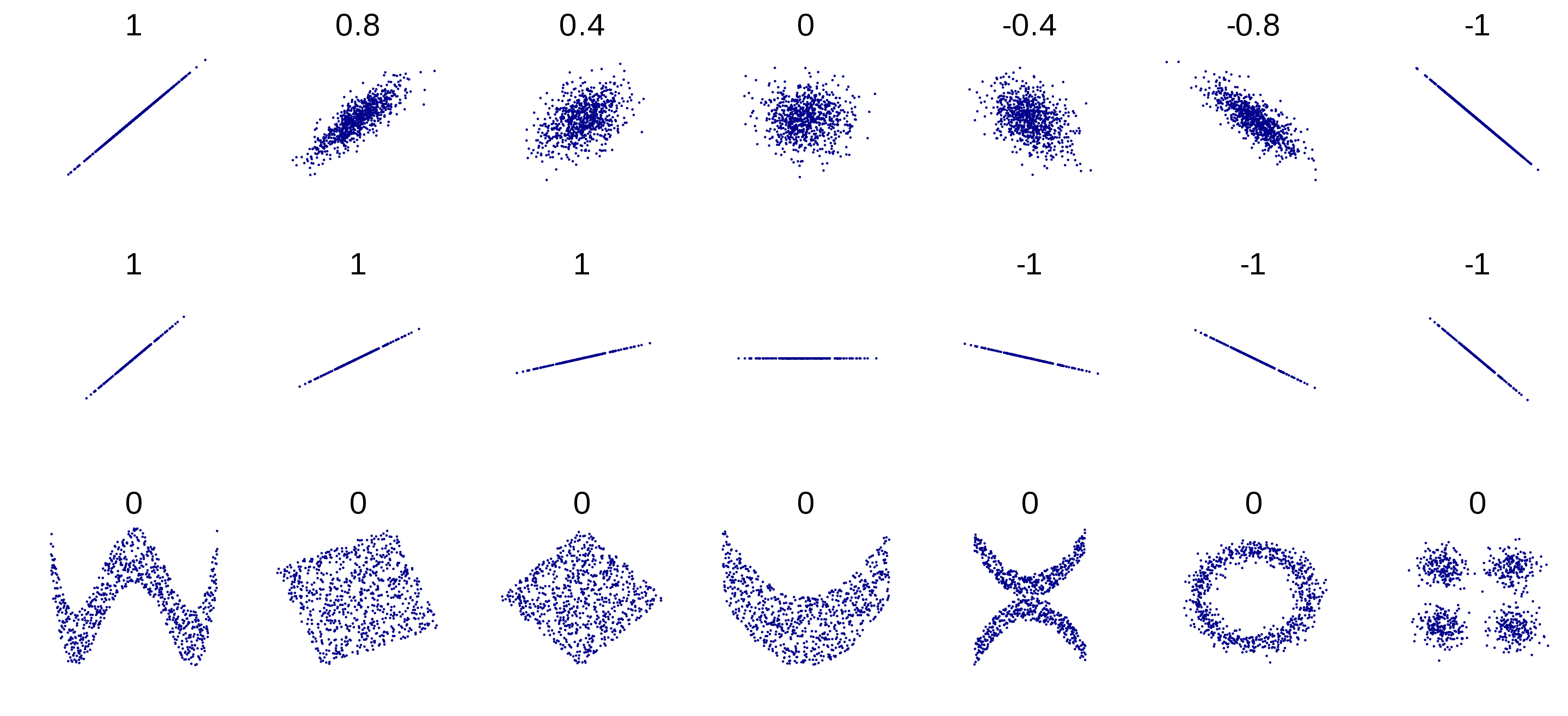
Several sets of (x, y) points, with the Pearson correlation coefficient of x and y for each set. The correlation reflects the noisiness and direction of a linear relationship (top row), but not the slope of that relationship (middle), nor many aspects of nonlinear relationships (bottom). N.B.: the figure in the center has a slope of 0 but in that case the correlation coefficient is undefined because the variance of Y is zero.
Reference: https://en.wikipedia.org/wiki/Correlation_and_dependence
Example: Colleges and Universities Data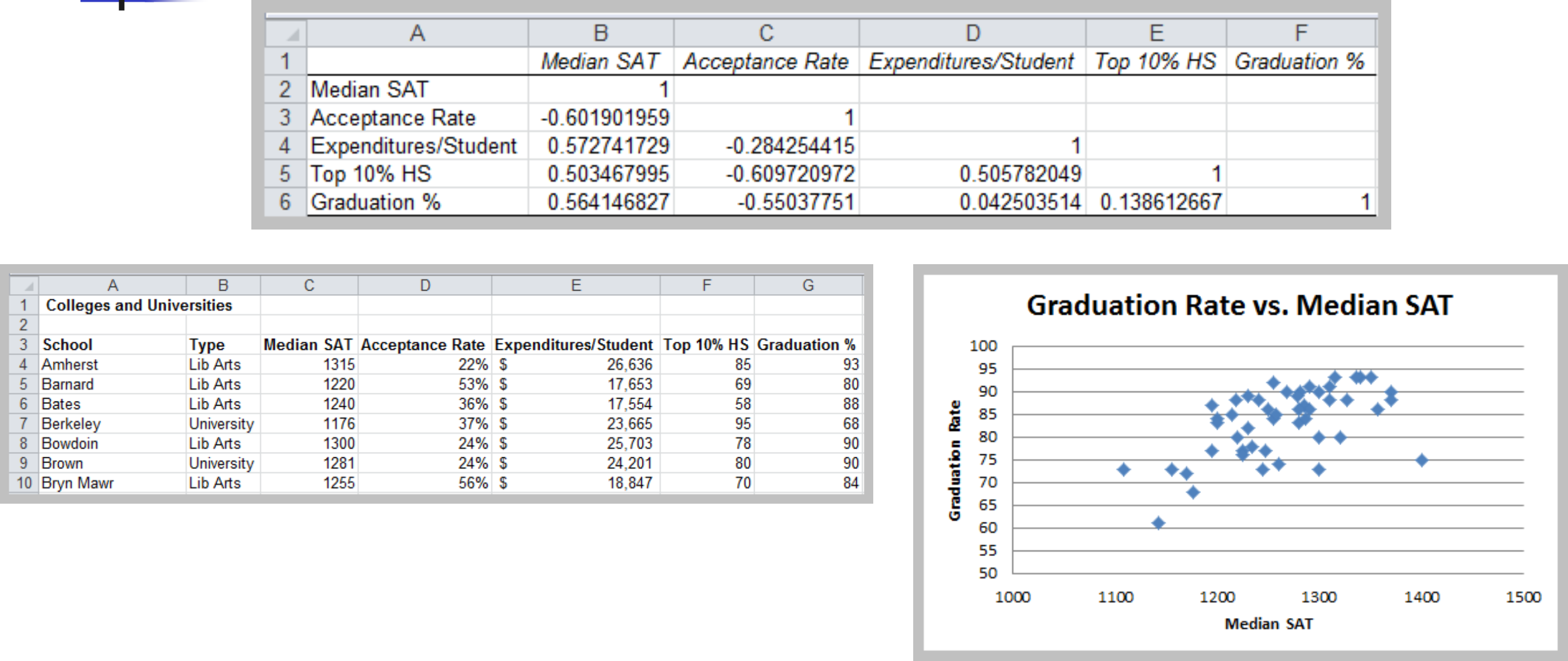
Correlation Coefficient in Python
1 | import pandas as pd |

Correlation Coefficient in Dataframe
1 | np.corrcoef(df['Height(inches)'][:100], df['Weight(pounds)'][:100]) |
Correlation Coefficient in ndarray
1 | np_baseball = np.array(df) |
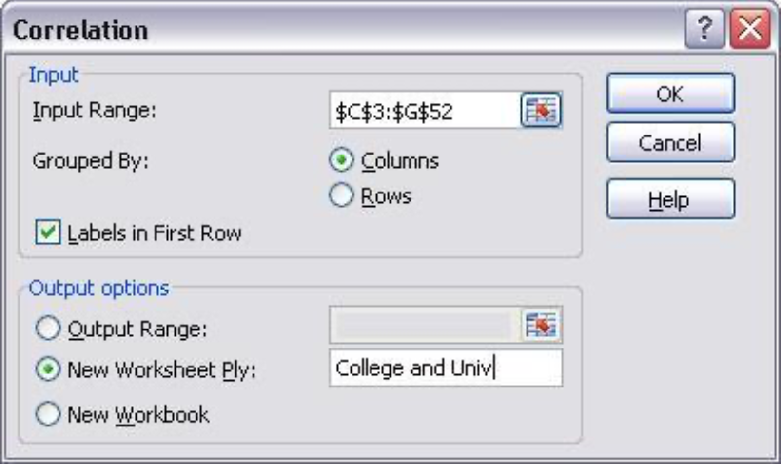
Excel Tool: Correlation
- Excel menu > Tools > Data Analysis > Correlation
Descriptive Statistics for Categorical Data
- Sample proportion, $p$ - fraction of data that has a certain characteristic
- Use the Excel function COUNTIF(data range, criteria) to count observations meeting a criterion to compute proportions.
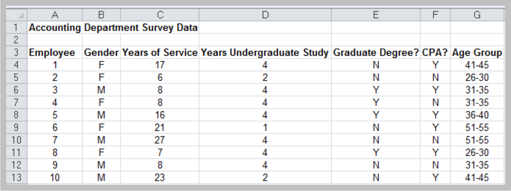
Cross-Tabulation (Contingency Table)
- A tabular method that displays the number of observations in a data set for different subcategories of two categorical variables.
- The subcategories of the variables must be mutually exclusive and exhaustive, meaning that each observation can be classified into only one subcategory and, taken together over all subcategories, they must constitute the complete data set.
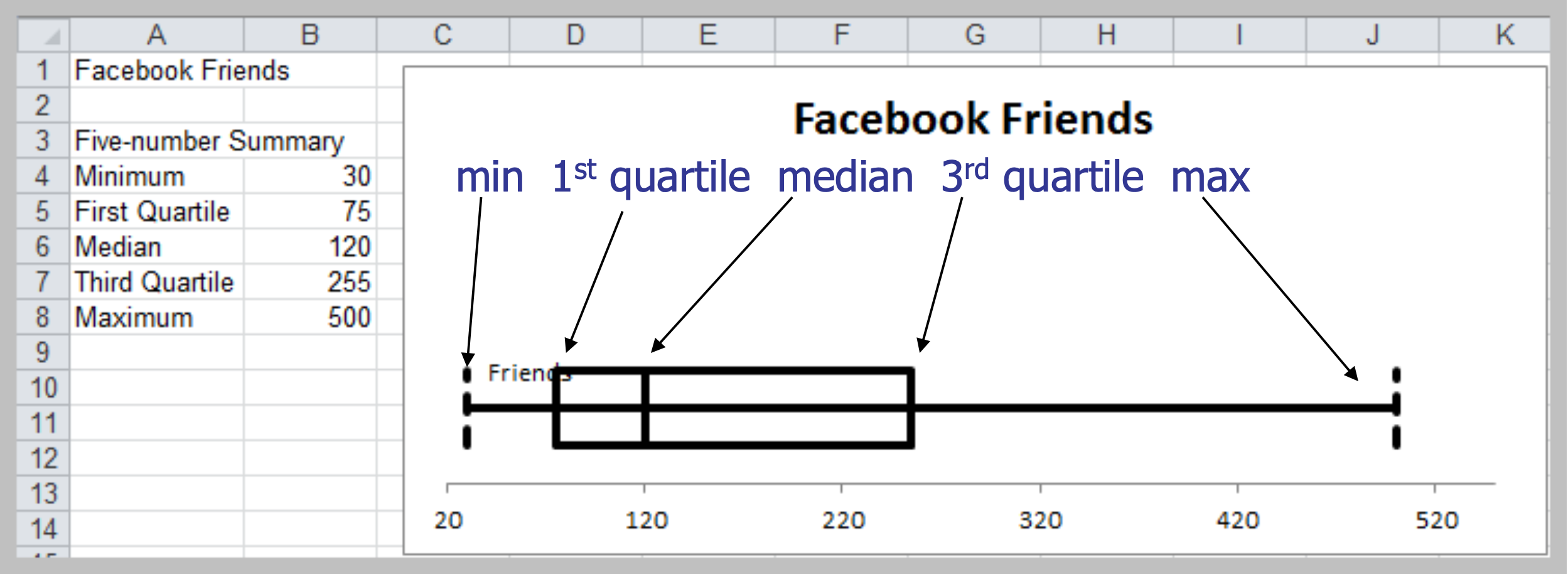
Example: Facebook Survey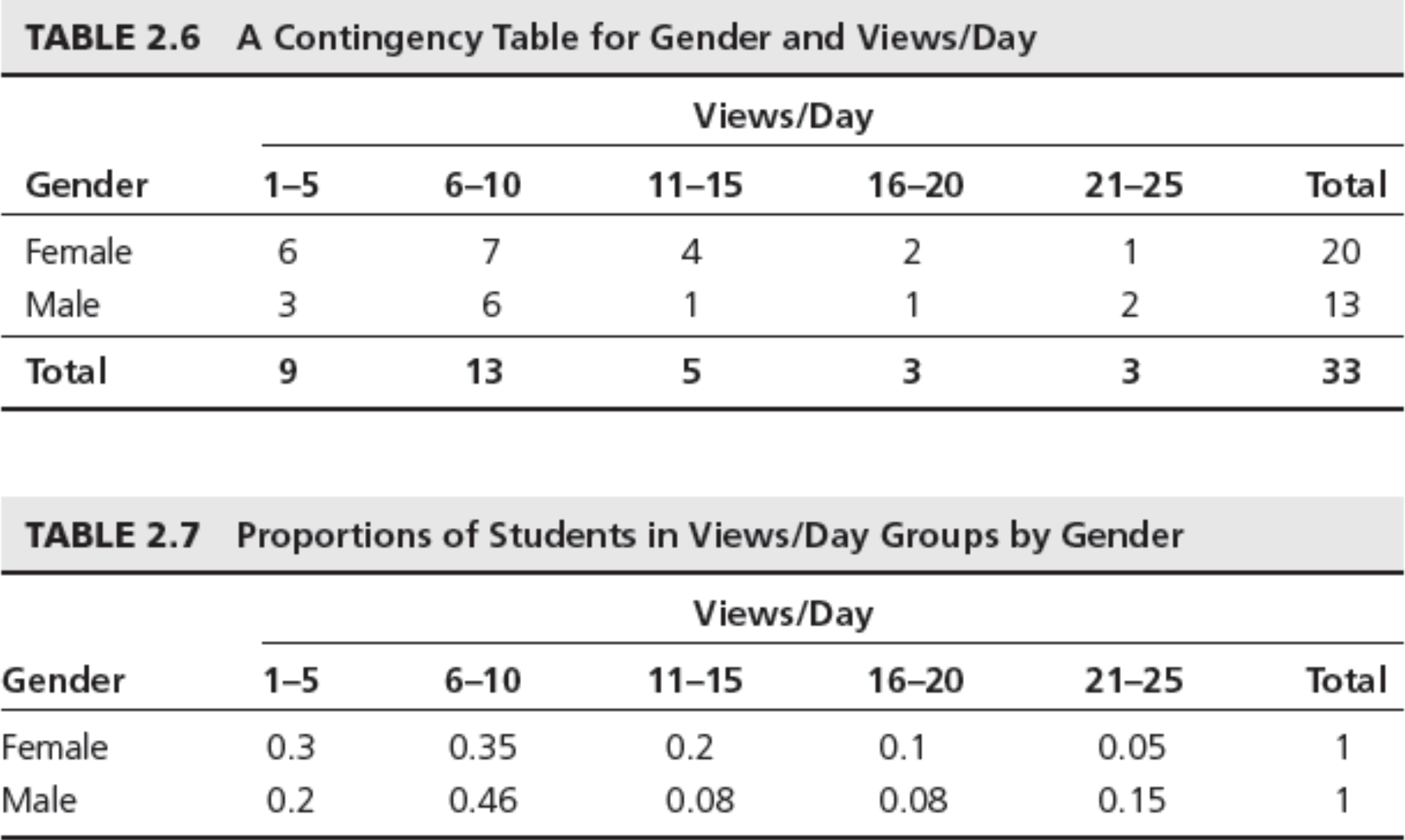
Data Analysis
Box Plots
- Display minimum, first quartile (Q1), median, third quartile (Q3), and maximum values graphically
Dot Scale Diagram
- PHStat menu > Descriptive Statistics > Dot Scale Diagram
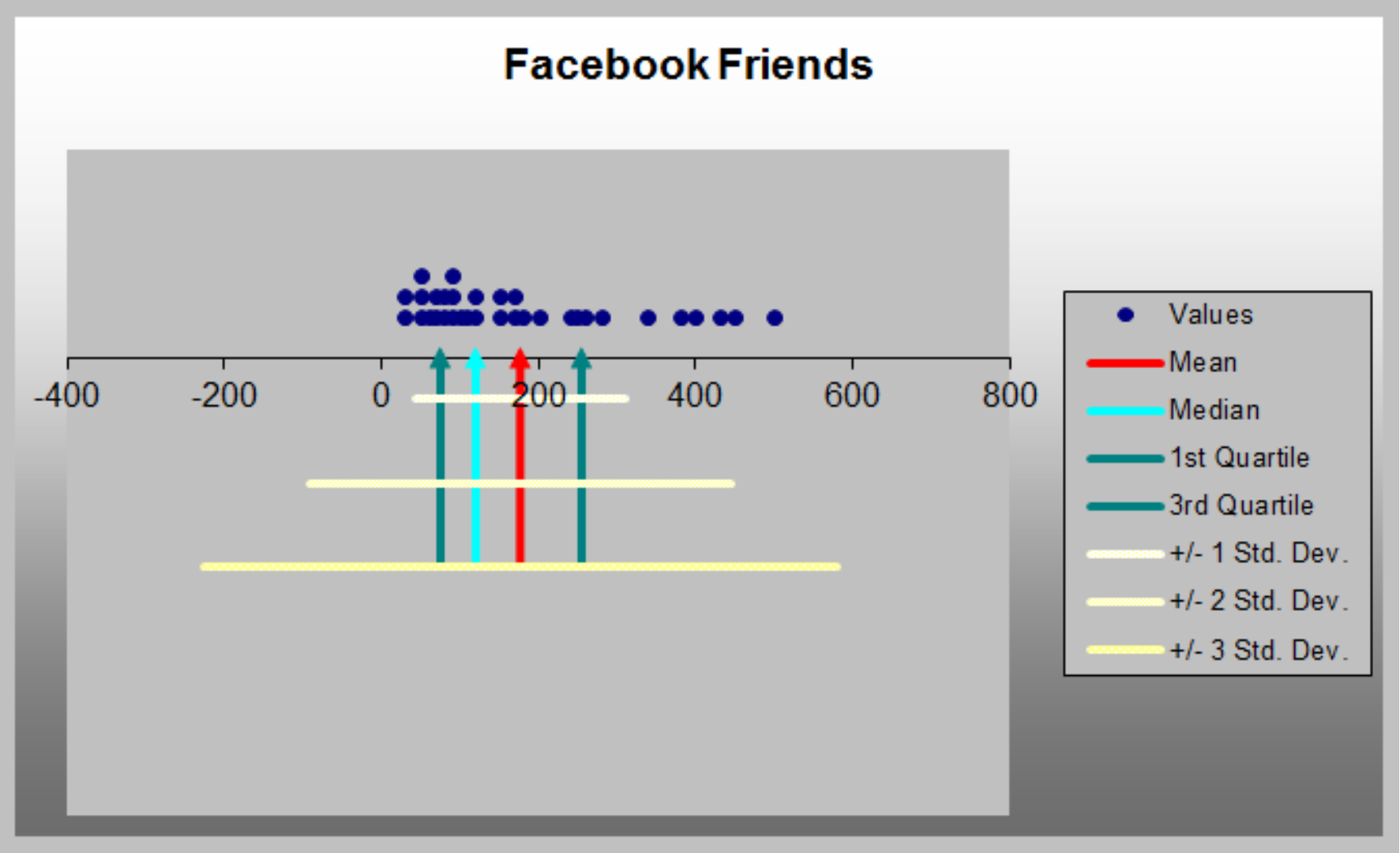
Outliers
- Outliers can make a significant difference in the results we obtain from statistical analyses.
- Box plots and dot‐scale diagrams can help identify possible outliers visually.
- Other approaches:
- Use the empirical rule to identify an outlier as one that is
more than three standard deviations from the mean. - Use the IQR. “Mild” outliers are often defined as being between $1.5 \times IQR$ and $3 \times IQR$ to the left of Q1 or to the right of Q3 , and “extreme” outliers as more than $3 \times IQR$ away from these quartiles.
- Use the empirical rule to identify an outlier as one that is
Pivot Table
- Create custom summaries and charts from data
- Need a data set with column labels. Select any cell and choose PivotTable Report from Data menu. Follow the wizard steps.
Blank PivotTable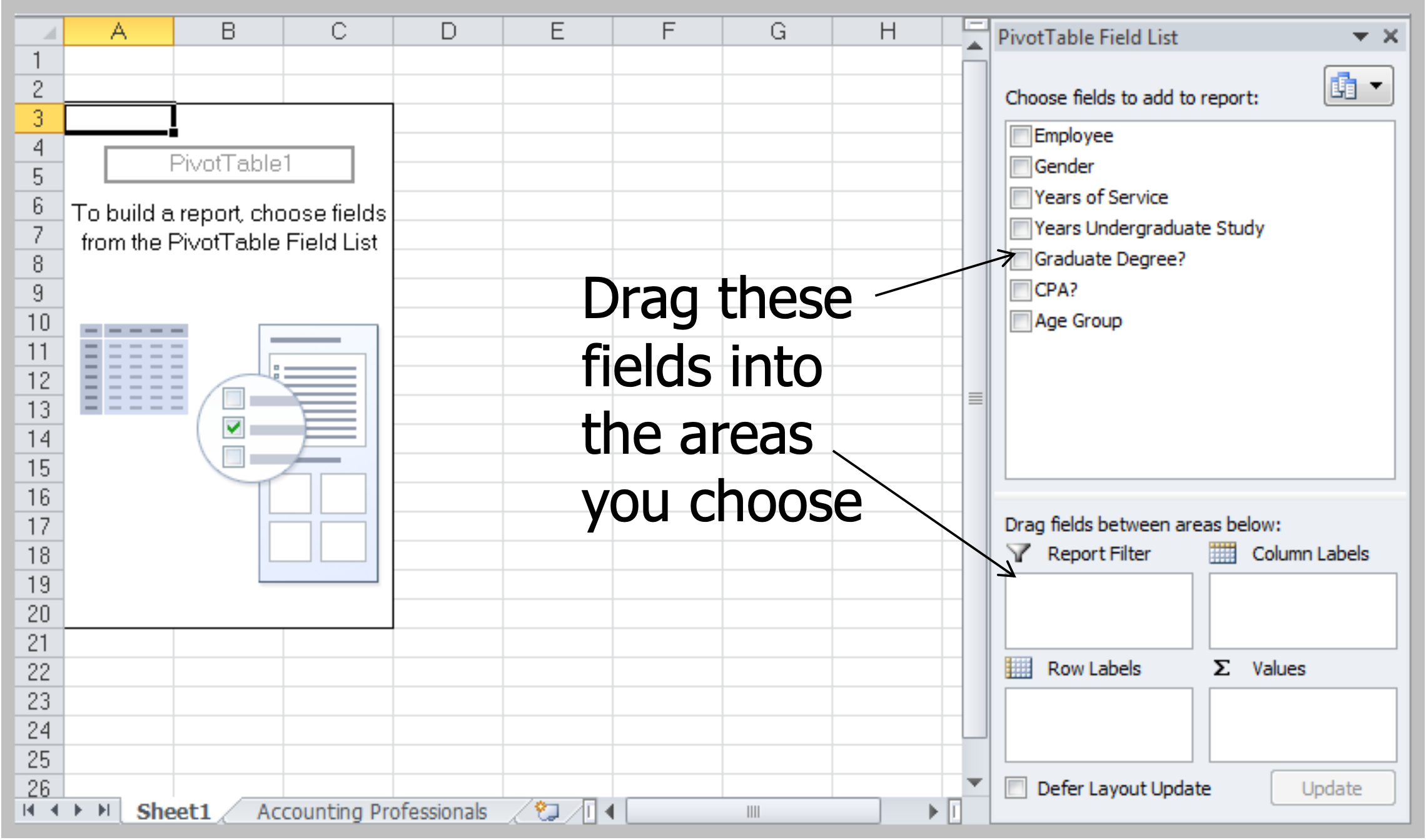
Excel PivotTable
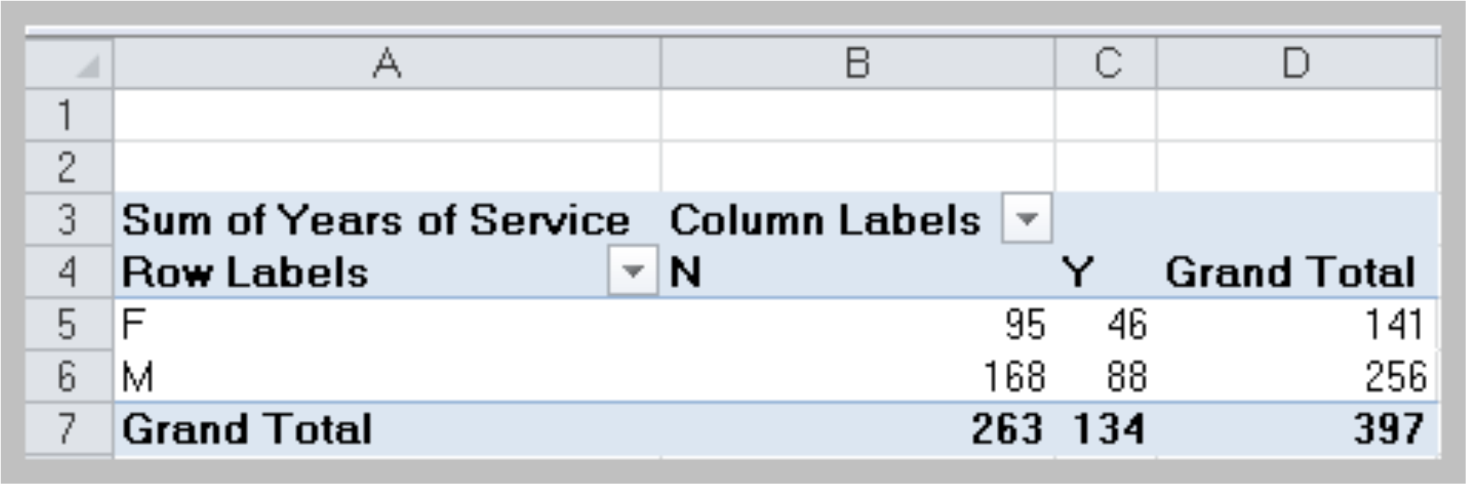
- Drag Gender from the PivotTable Field List to the Row Labels area, Graduate Degree? into the Column Labels area, and Years of Service into the Values area:
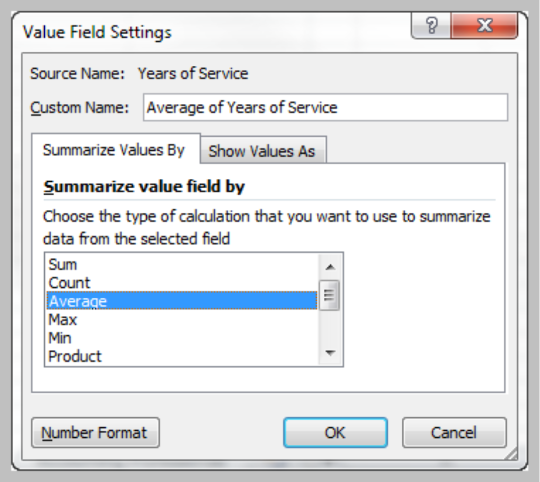
Value Field Settings
- In the Options tab under PivotTable Tools in the menu bar, click on the Active Field group and choose Value Field Settings to change type of summary
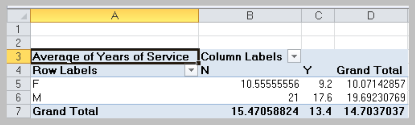
Changing PivotTable Views
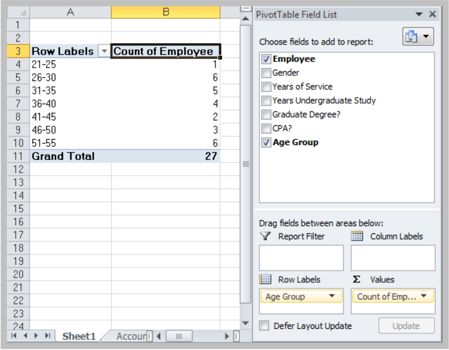
Uncheck the boxes in the PivotTable Field List or drag the variable names to different field areas.
PivotTables for Cross Tabulation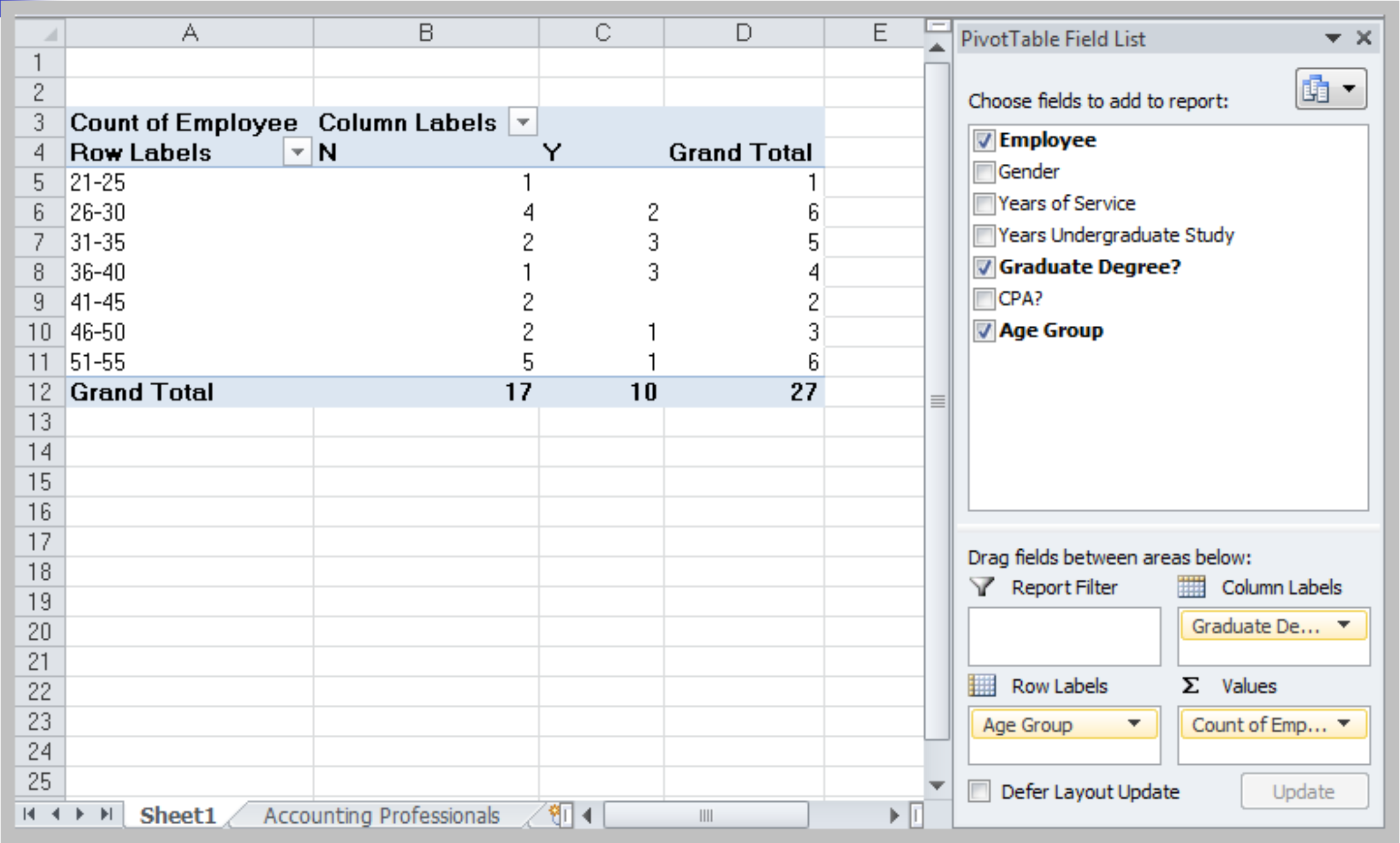
Grouped Data
Grouped data are data formed by aggregating individual observations of a variable into groups, so that a frequency distribution of these groups serves as a convenient means of summarizing or analyzing the data.
Grouped Data: Calculation of Mean
- Sample: $\displaystyle \bar x = \frac{\sum^n_{i=1}f_i x_i}{n}$
- Population: $\displaystyle \mu = \frac{\sum^n_{i=1}f_i x_i}{N}$
Example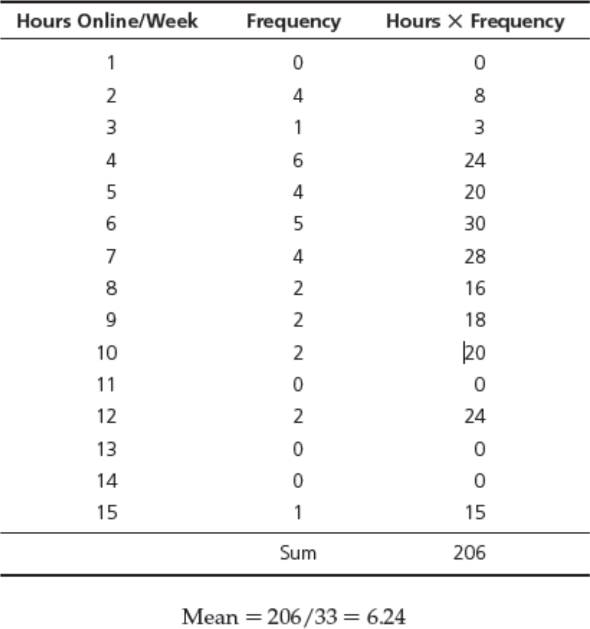
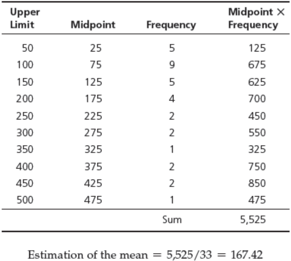
Grouped Frequency Distribution
- We may estimate the mean by replacing $x_i$ with a representative value (such as the midpoint) for all the observations in each cell.
Grouped Data: Calculation of Variance
- Sample: $\displaystyle s^2 = \frac{\sum^n_{i=1}f_i(x_i-\bar x)^2}{n-1}$
- Sample: $\displaystyle \sigma ^2 = \frac{\sum^n_{i=1}f_i(x_i-\mu)^2}{N}$
CHAPTER 3: PROBABILITY CONCEPTS AND DISTRIBUTIONS
Probability
- Probability – the likelihood that an outcome occurs
- Probabilities are values between 0 and 1. The closer the probability is to 1, the more likely it is that the outcome will occur.
- Some convert probabilities to percentages
- The statement “there is a 10% chance that oil prices will rise next quarter” is another way of stating that “the probability of a rise in oil prices is 0.1.”
Experiments and Outcomes
Experiment – a process that results in some outcome
- Roll dice
- Observe and record weather conditions
- Conduct market survey
- Watch the stock market
- Outcome – an observed result of an experiment
- Sum of the dice
- Description of the weather
- Proportion of respondents who favor a product
- Change in the Dow Jones Industrial Average
Sample Space
- Sample space - all possible outcomes of an experiment
- Dice rolls: 2, 3, …, 12
- Weather outcomes: clear, partly cloudy,
cloudy - Customer reaction: proportion who favor a product (a number between 0 and 1)
- Change in DJIA: positive or negative real number
Three Views of Probability
- Classical definition: based on theory
- Relative frequency: based on empirical
data - Subjective: based on judgment
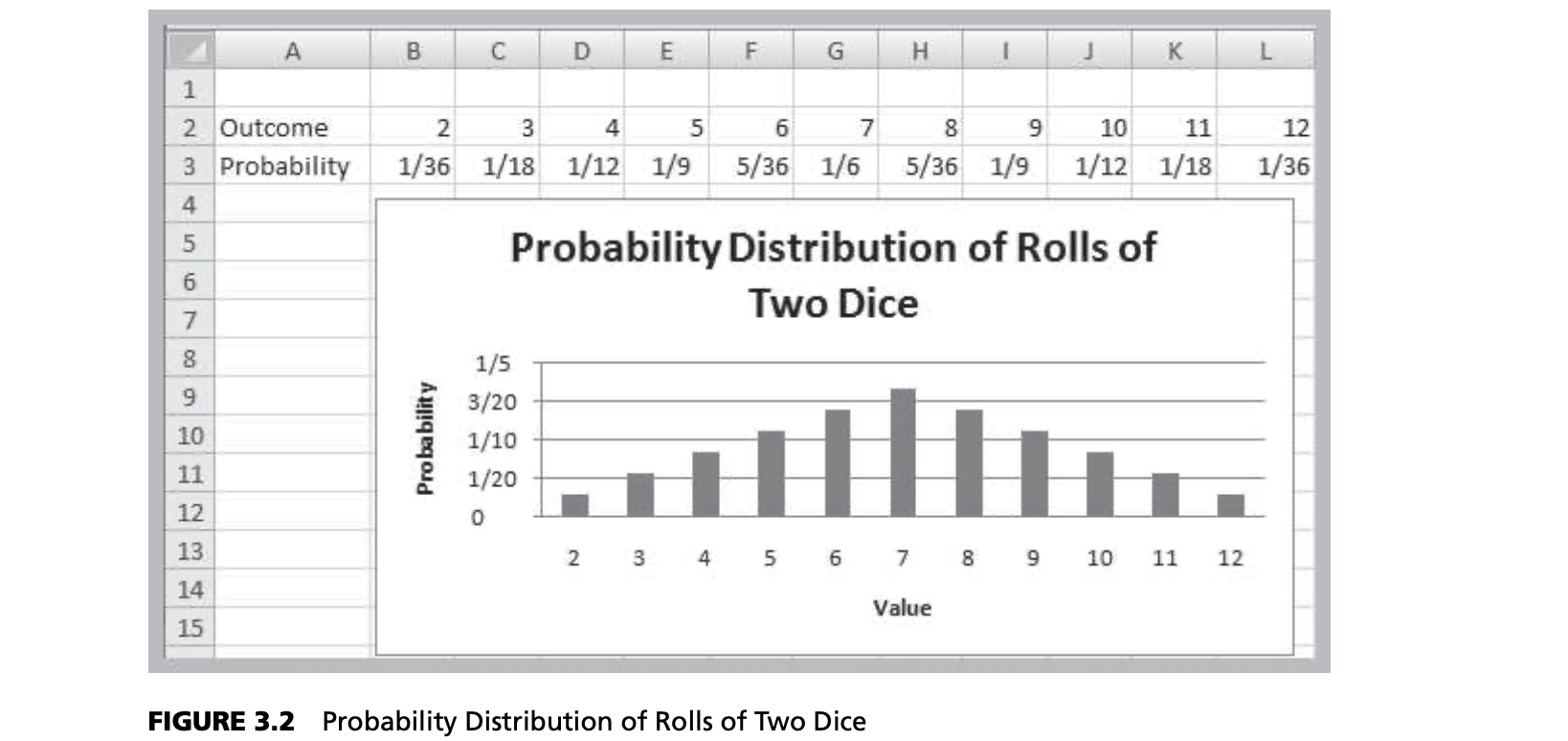
Classical Definition
- Probability = number of favorable outcomes divided by the total number of possible outcomes
- Example: There are six ways of rolling a 7 with a pair of dice, and 36 possible rolls. Therefore, the probability of rolling a 7 is 6/36 = 0.167.
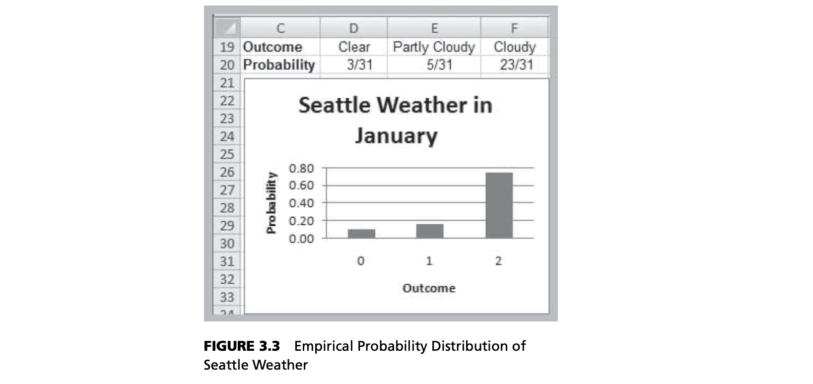
Relative Frequency Definition
- Probability = number of times an event has occurred in the past divided by the total number of observations
- Example: Of the last 10 days when certain weather conditions have been observed, it has rained the next day 8 times. The probability of rain the next day is 0.80
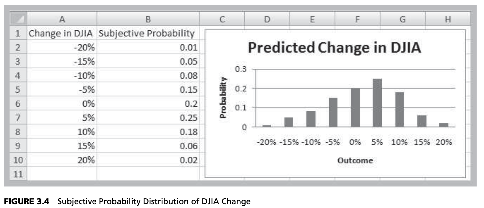
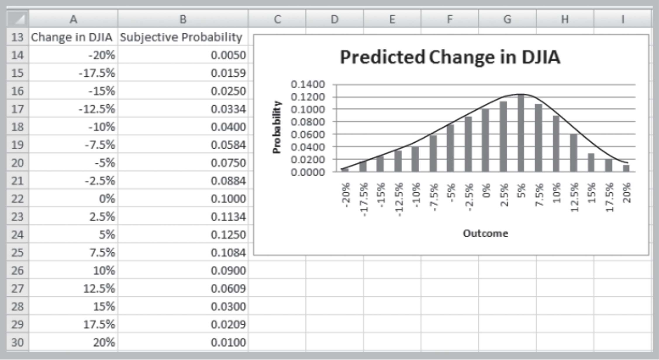
Subjective Definition
- What is the probability that the New York Yankees will win the World Series this year?
- What is the probability your school will win its conference championship this year?
- What is the probability the NASDAQ will go up 2% next week?
Basic Probability Rules and Formulas
- Probability associated with any outcome must be between 0 and 1
- $0 ≤ P(O_i) ≤ 1$ for each outcome $O_i$
- Sum of probabilities over all possible outcomes must be
$1$- $P(O_1)+P(O_2)+…+P(O_n)$ =1
- Example: Flip a coin three times
- Outcomes: HHH, HHT, HTH, THH, HTT, THT, TTH, TTT Each has probability of (1/2)3 = 1/8
Events
- An event is a collection of one or more outcomes from
- Obtaining a 7 or 11 on a roll of dice
- Having a clear or partly cloudy day
- The proportion of respondents that favor a product is at least 0.60
- Having a positive weekly change in the Dow
- If $A$ is any event, the complement of $A$, denoted $A^c$, consists of all outcomes in the sample space not in $A$.
Rules
- The probability of any event is the sum of the probabilities of the outcomes that compose that event.
- The probability of the complement of any event $A$ is $P(A^c) = 1 - P(A)$.
- If events A and B are mutually exclusive, then
- $P(A \cup B) = P(A) + P(B)$.
- If two events A and B are not mutually exclusive, then
- $P(A \cup B) = P(A) + P(B) - P(A \cap B)$.
Mutually Exclusive Events
- Two events are mutually exclusive if they have no outcomes in common.
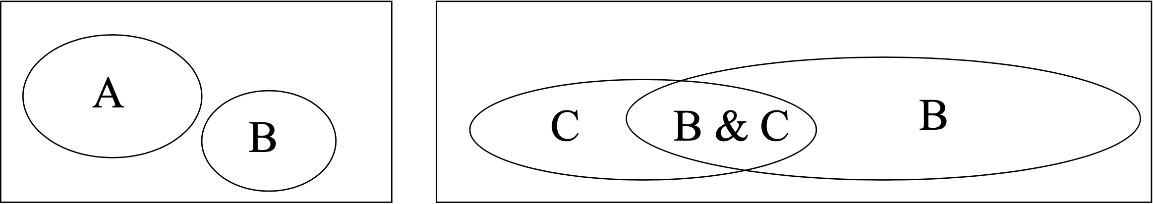
- A and B are mutually exclusive
- B and C are not mutually exclusive
Example
- What is the probability of obtaining exactly two heads or exactly two tails in 3 flips of a coin?
- These events are mutually exclusive. Probability = 3/8 + 3/8 = 6/8
- What is the probability of obtaining at least two tails or at least one head?
- $A = {TTT, TTH, THT, HTT}$, $B = {TTH, THT, THH, HTT, HTH, HHT, HHH}$. The events are not mutually exclusive.
- $P(A) = 4/8$; $P(B) = 7/8$; $P(A \cap B) = 3/8$. Therefore, $P(A \cup B) = 4/8 + 7/8 – 3/8 = 1$
Conditional Probability
- Conditional probability – the probability of the occurrence of one event, A, given that another event B is known to be true or have already occurred.
- $P(A|B) = P(A \cap B)/P(B)$
Example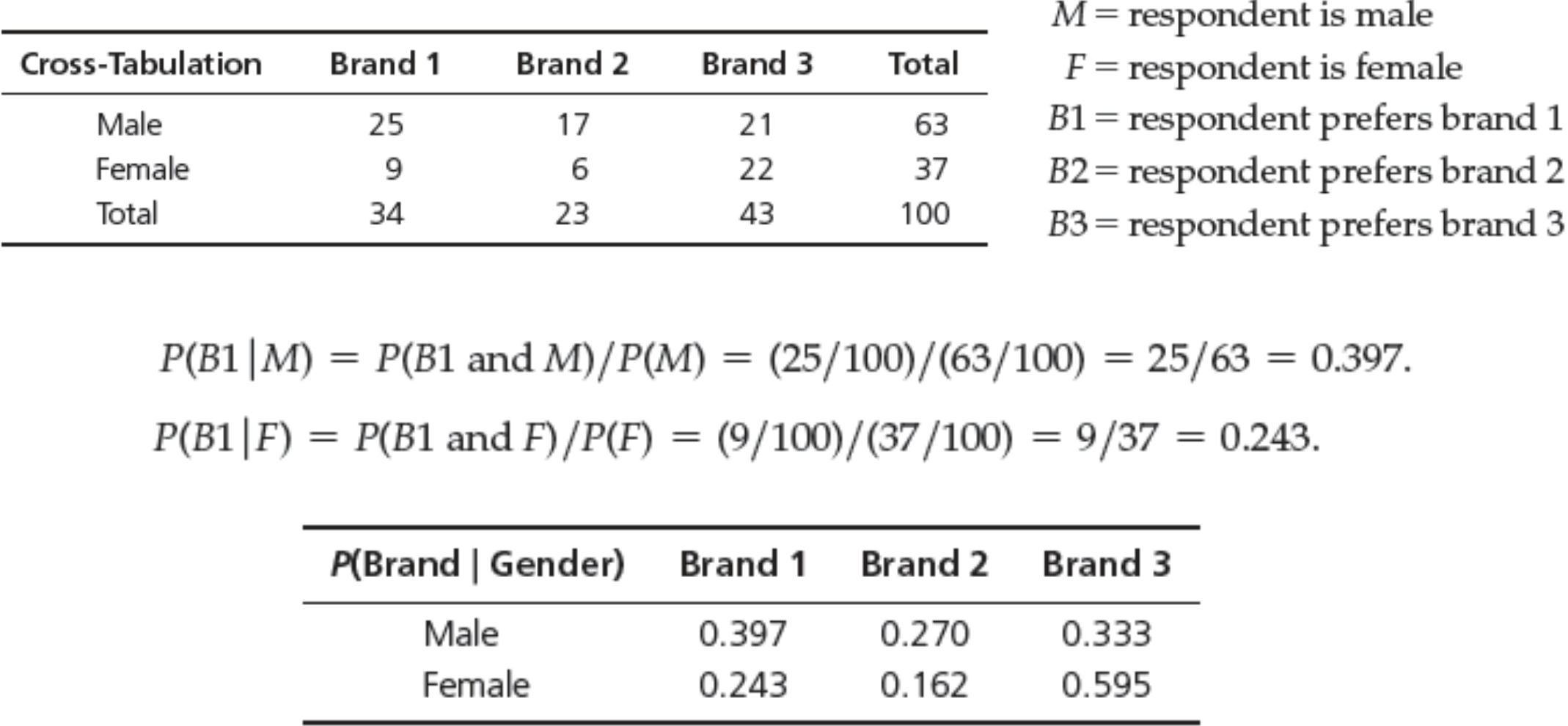
Multiplication Law of Probability
- $P(A \cap B) = P(A |B) P(B) = P(B |A) P(A)$
- Two events A and B are independent if $P(A |B) = P(A)$
- If A and B are independent, then
- $P(A \cap B) = P(B)P(A) = P(A)P(B)$
Random Variables and Probability Distributions
- Random variable: a numerical description of the outcome of an experiment. Random variables are denoted by capital letters, $X$, $Y$, …; specific values by lower case letters, $x$, $y$, …
- Discrete random variable: the number of possible outcomes can be counted
- Continuous random variable: outcomes over one or more continuous intervals of real numbers
Example
- Experiment: flip a coin 3 times.
- Outcomes: TTT, TTH, THT, THH, HTT, HTH, HHT,
HHH - Random variable: X = number of heads.
- $X$ can be either 0, 1, 2, or 3.
- Experiment: observe end-of-week closing stock price.
- Random variable: $Y$ = closing stock price.
- $X$ can be any nonnegative real number.
Probability Distributions
- Probability distribution: a characterization of the possible values a random variable may assume along with the probability of assuming these values.
- Probability distributions may be defined for both discrete and continuous random variables.
Discrete Random Variables
- Probability mass function $f(x)$: specifies the probability of each discrete outcome
- Two properties:
- $0 \le f(x_i) \le 1$ for all $i$
- $\sum_i{f(x_i)=1}$
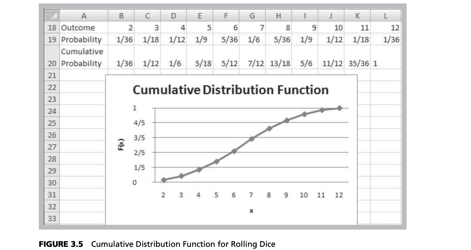
Cumulative Distribution Function, $F(x)$
- Specifies the probability that the random variable $X$ will be less than or equal to $x$, denoted as $P(X ≤ x)$.
Expected Value and Variance of Discrete Random Variables
- Expected value of a random variable $X$ is the theoretical analogy of the mean, or weighted average of possible values:
$$E[X] = \sum_{i=1}^\infty x_i f(x_i)$$ - Variance and standard deviation of a random variable $X$:
$$V[X] = \sum_{j=1}^\infty (x - E(X)^2f(x)$$
$$\sigma_X = \sqrt{\sum_{j=1}^\infty (x_j - E(X)^2f(x_j)}$$
Discrete Probability
- Bernoulli
- Binomial
- Poisson
Bernoulli Distribution
- A random variable with two possible outcomes: “success” $(x = 0)$ and “failure” $(x = 1)$
- $p$ = probability of “success”
$$y=\begin{cases}
p,\quad &if \space x = 1 \
1-p, &if \space x = 0
\end{cases}$$
- Expected value = $p$; variance = $p(1 – p)$
Binomial Distribution
- $n$ independent replications of a Bernoulli experiment, each with constant probability of success $p$
- $X$ represents the number of successes in $n$ experiments.
- Expected value = $np$
- Variance = $np(1-p)$
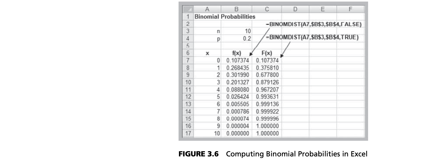
Example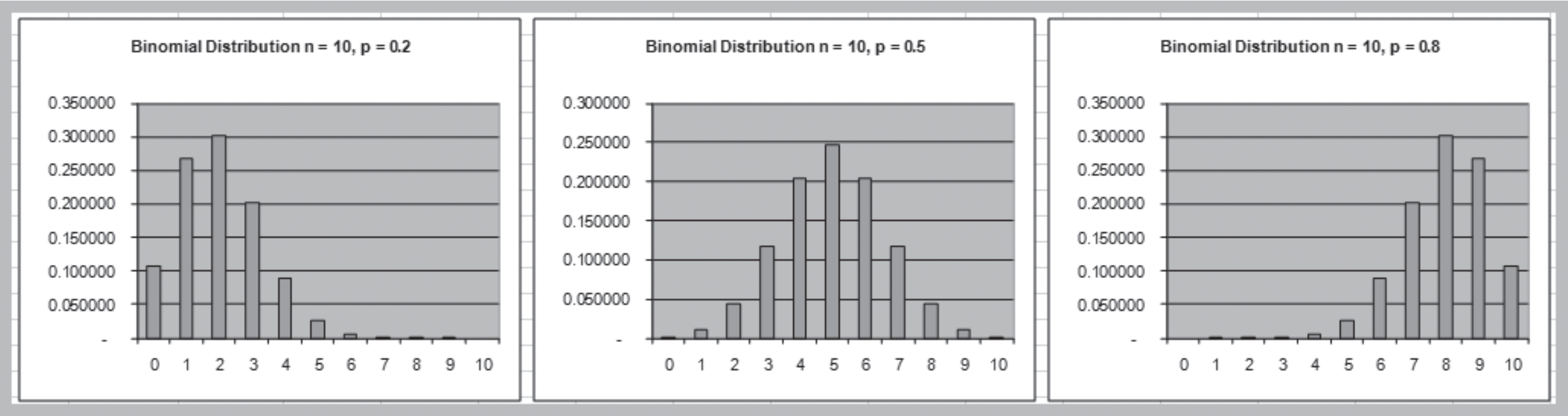
Excel Function
- BINOM.DIST(number_s, trials, probability_s, cumulative)
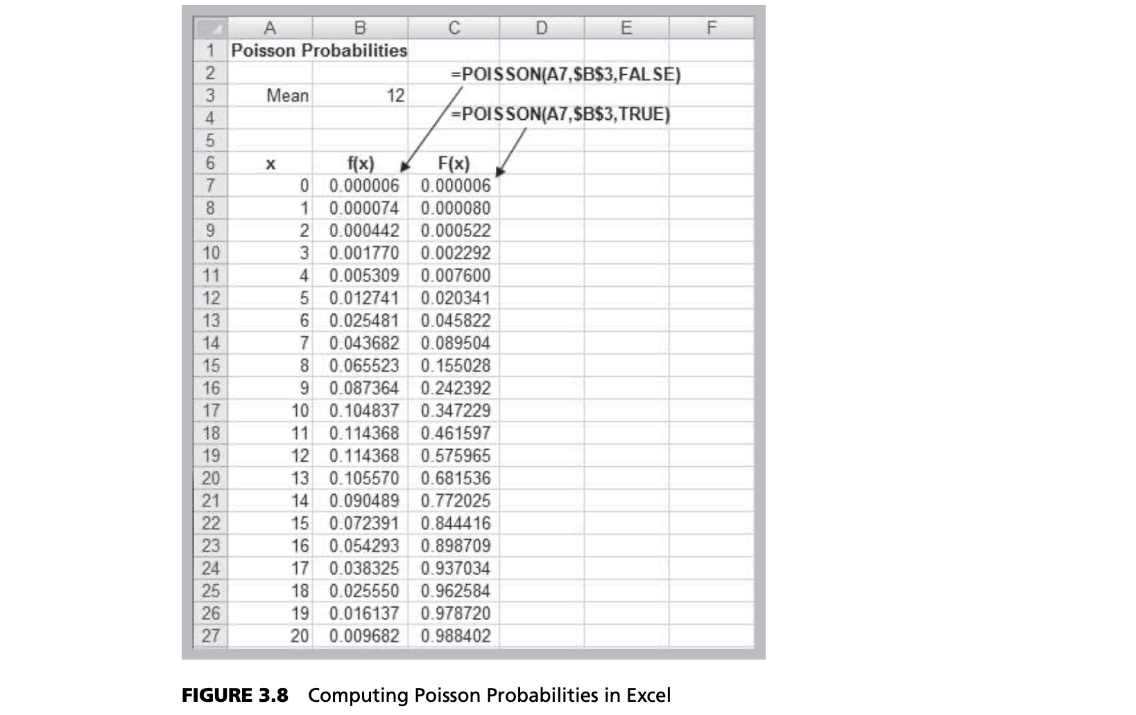
Poisson Distribution
- Models the number of occurrences in some unit of measure, e.g., events per unit time, number of items per order
- $X$ = number of events that occur; $x = 0, 1, 2$,
- Expected value = $\lambda$; variance = $\lambda$
- Poisson approximates binomial when $n$ is very large and $p$ is very small
$$\displaystyle \lim_{n \to +\infty, p \to 0} np = undefined = \lambda$$
Example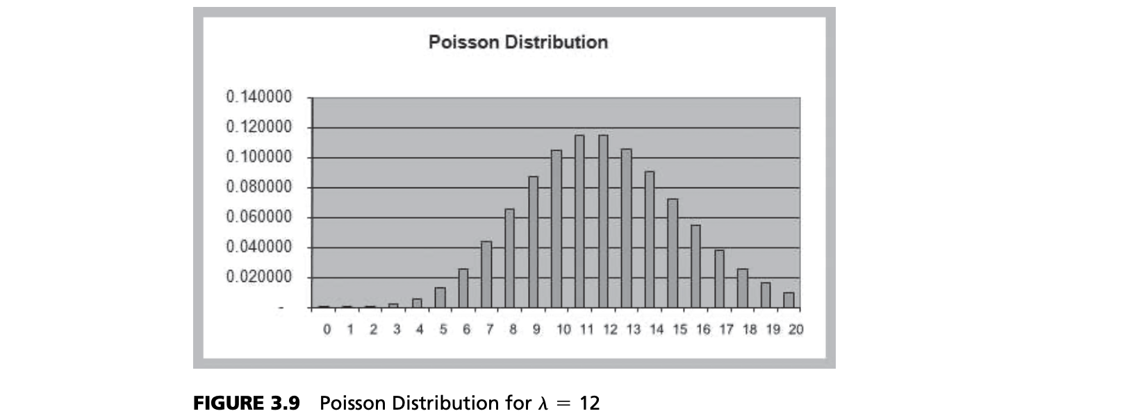
Excel function
- POISSON.DIST(x, mean, cumulative)
CONTINUOUS PROBABILITY DISTRIBUTIONS
- Probability density function, $f(x)$, a continuous function that describes the probability of outcomes for a continuous random variable $X$. A histogram of sample data approximates the shape of the underlying density function.
Refining Subjective Probabilities Toward a Continuous Distribution
Properties of Probability Density Functions
- $f(x) \ge 0$ for all $x$
- Total area under $f(x) = 1$
- There are always infinitely many values for $X$
- $P(X = x) = 0$[372]
- We can only define probabilities over intervals:
$P(a ≤ X ≤ b), P(X < c), or \space P(X > d)$
Cumulative Distribution Function
- $F(x)$ specifies the probability that the random variable $X$ will be less than or equal to $x$; that is, $P(X \le x)$.
- $F(x)$ is equal to the area under f(x) to the left of $x$
- The probability that $X$ is between $a$ and $b$ is the area under $f(x)$ from a to b:
$$P(a ≤ X ≤ b) = P(X ≤ b) - P(X ≤ a) = F(b) – F(a)$$
Example
Properties of Continuous Distributions
- Continuous distributions have one or more parameters that characterize the density function:
- Shape parameter: controls the shape of the distribution
- Scale parameter: controls the unit of measurement
- Location parameter: specifies the location relative to zero on the horizontal axis
Uniform Distribution
- $EV[X] = (a + b)/2$
- $V[X] = (b – a)^2/12$
- a = location
- b = scale for fixed a

Normal Distribution
- Familiar bell-shaped curve.
- Symmetric, median = mean = mode; half the area is on
either side of the mean - Range is unbounded: the curve never touches the x-axis Parameters
- Mean, $\mu $ (the location parameter)
- Variance $\sigma^2 > 0$ (the location parameter)
- Density function: $\displaystyle \frac{e^{-\frac{(x-\mu)^2}{2\sigma^2}}}{\sqrt{2\pi \sigma^2}}$
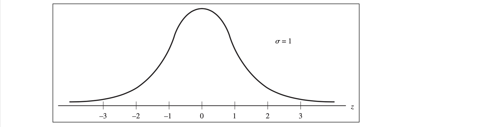
Standard Normal Distribution
- Standard Normal Distribution when $\mu = 0, \space \sigma^2 = 1$, denoted as $N(0,1)$
- if $X \sim N(\mu, \sigma^2)$, then $\displaystyle Z = \frac{(X - \mu)}{\sigma} \sim N(0, 1)$
Excel Functions
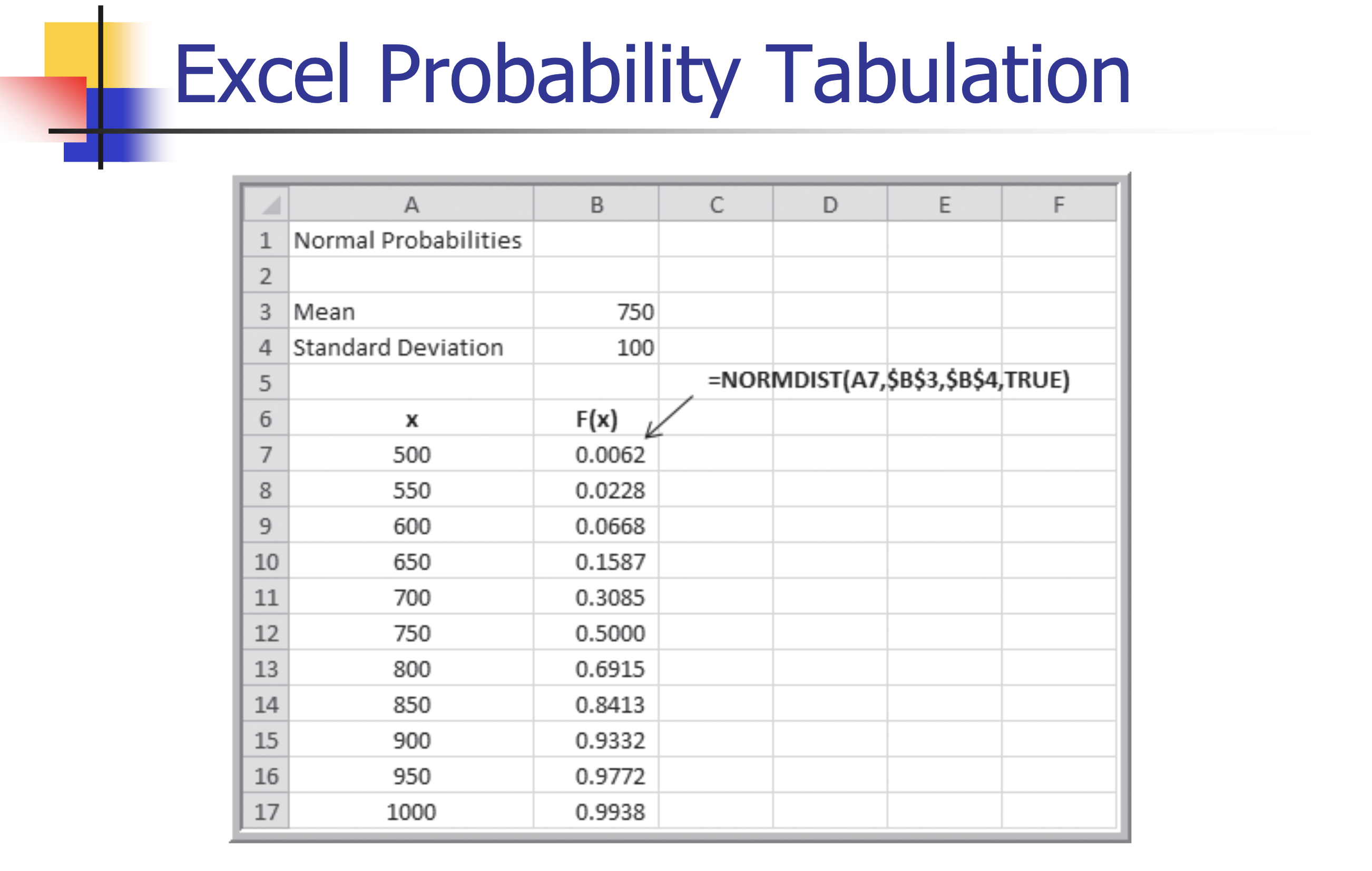
- NORM.DIST(x, mean, standard_deviation, cumulative)
- NORM.DIST(x, mean, standard_deviation, TRUE)[3762] calculates the cumulative probability $F(x) = P(X \le x)$ for a specified mean and standard deviation.
- NORM.S.DIST(z)
- NORM.S.DIST(z) generates the cumulative probability for a standard normal distribution.
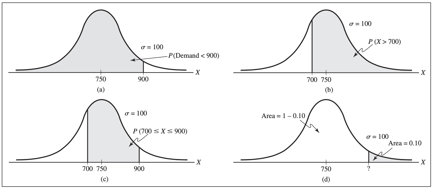
Example
- Customer demand $(X)$ is normal with a mean of 750 units/month and a standard deviation of 100 units/month.
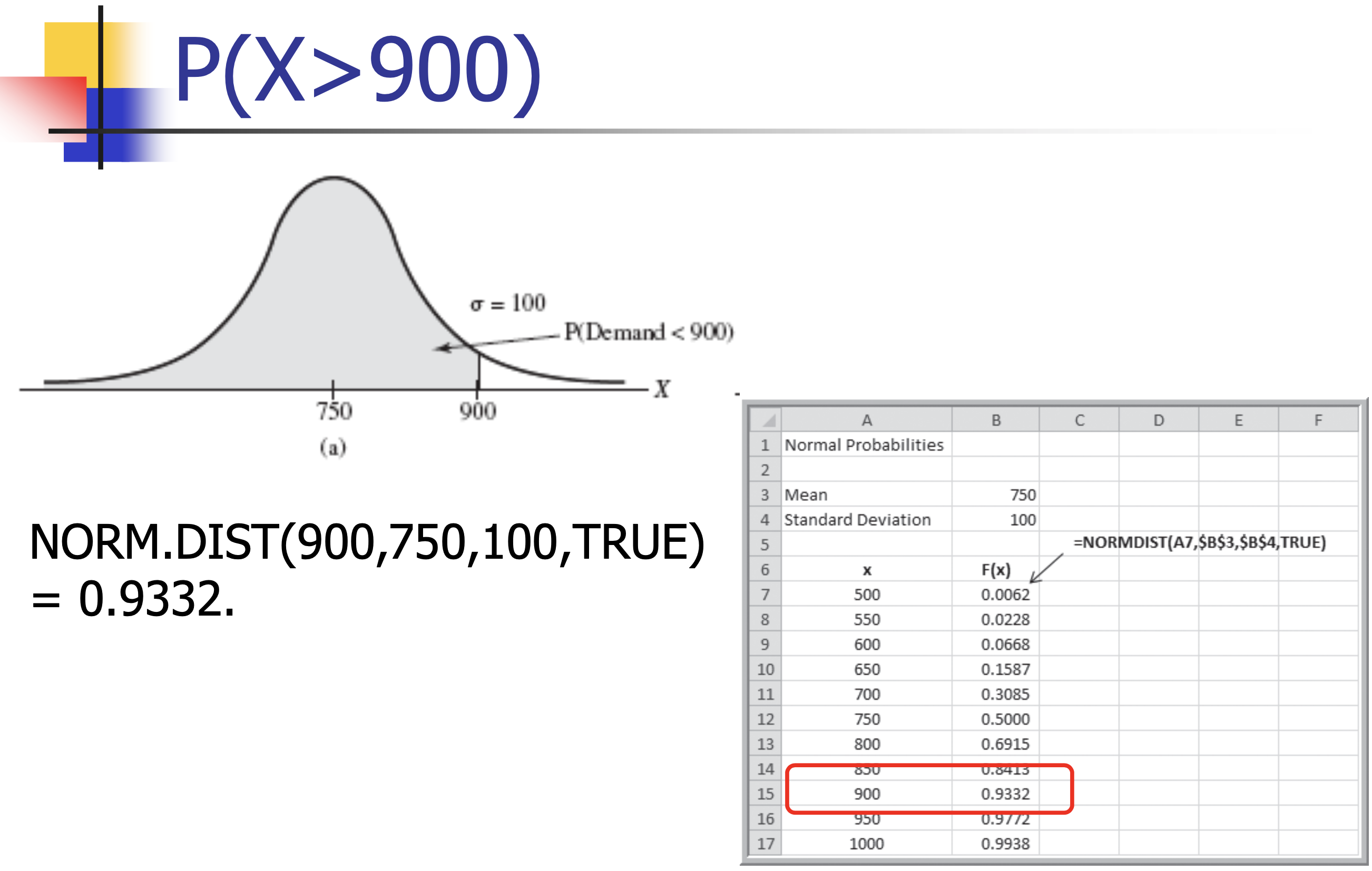
- What is the probability that demand will be at most 900 units?
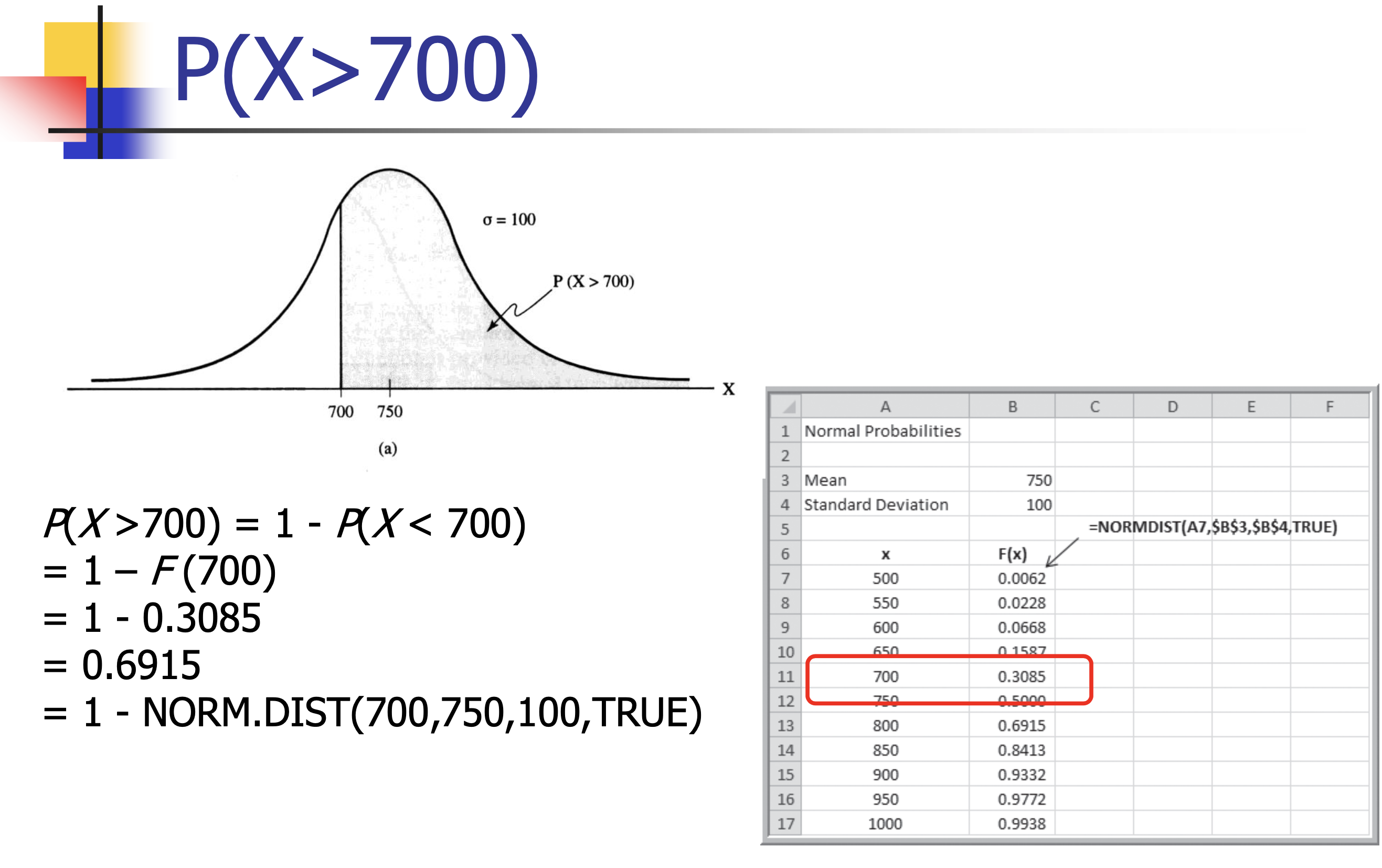
- What is the probability that demand will exceed 700 units?
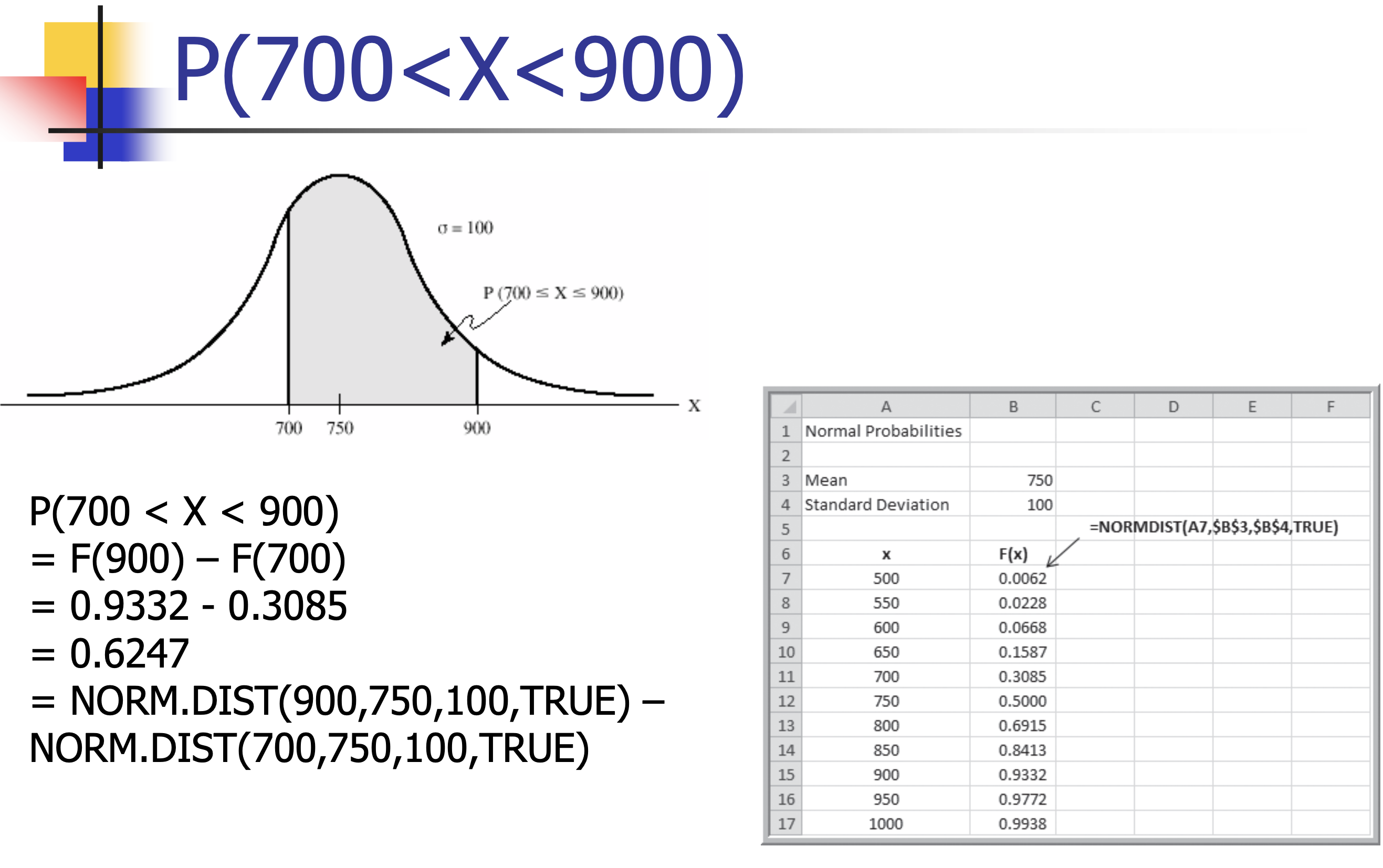
- What is the probability that demand will be between 700 and 900 units?
- What level of demand would be exceeded at most 10%
of the time?
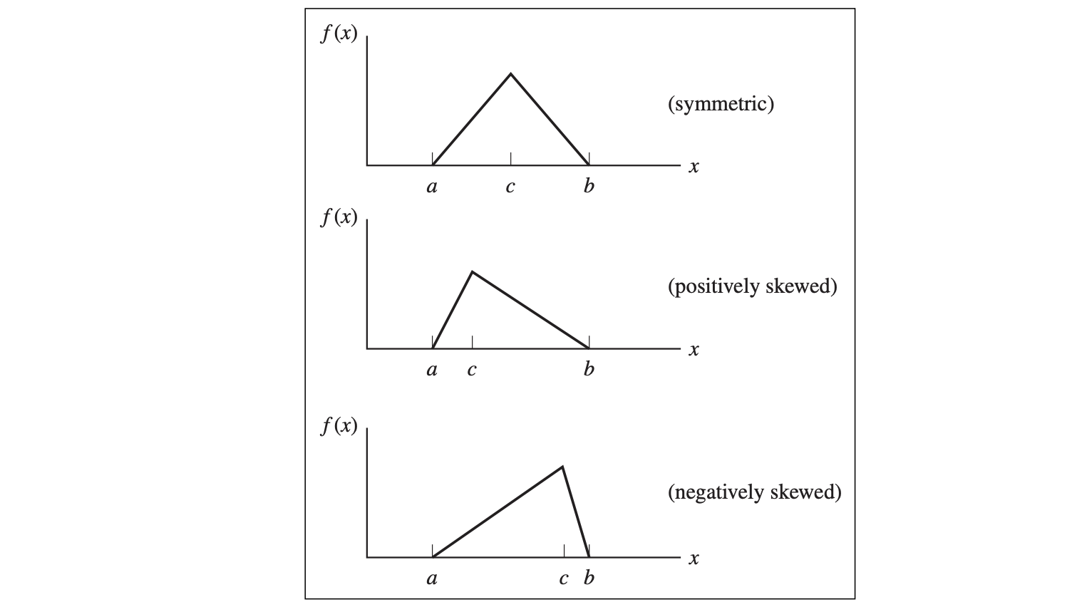
Triangular Distribution[377]
- Three parameters:
- Minimum, a
- Maximum, b
- Most likely, c[3771]
- a is the location parameter;
- b is the scale parameter for fixed a;
- c is the shape parameter.
- $EV[X] = (a + b + c)/3$
- $Var[X]=(a^2 +b^2 +c^2 -ab-ac-bc)/18$
Exponential Distribution
- Models events that occur randomly over time
- e.g., Customer arrivals, machine failures
- A key property of the exponential distribution is that it is memoryless; that is, the current time has no effect on future outcomes.
- For example, the length of time until a machine failure has the same distribution no matter how long the machine has been running.
Similar to the Poisson distribution, the exponential distribution has one parameter $\lambda$. In fact, the exponential distribution is closely related to the Poisson; if the number of events occurring during an interval of time has a Poisson distribution, then the time between events is exponentially distributed. For instance, if the number of arrivals at a bank is Poisson distributed, say with mean 12/hour, then the time between arrivals is exponential, with mean 1/12 hour, or 5 minutes.
Properties of Exponential
- $\lambda$, the scale parameter
- $EV[X] = 1/\lambda$
- $V[X] = 1/\lambda^2$
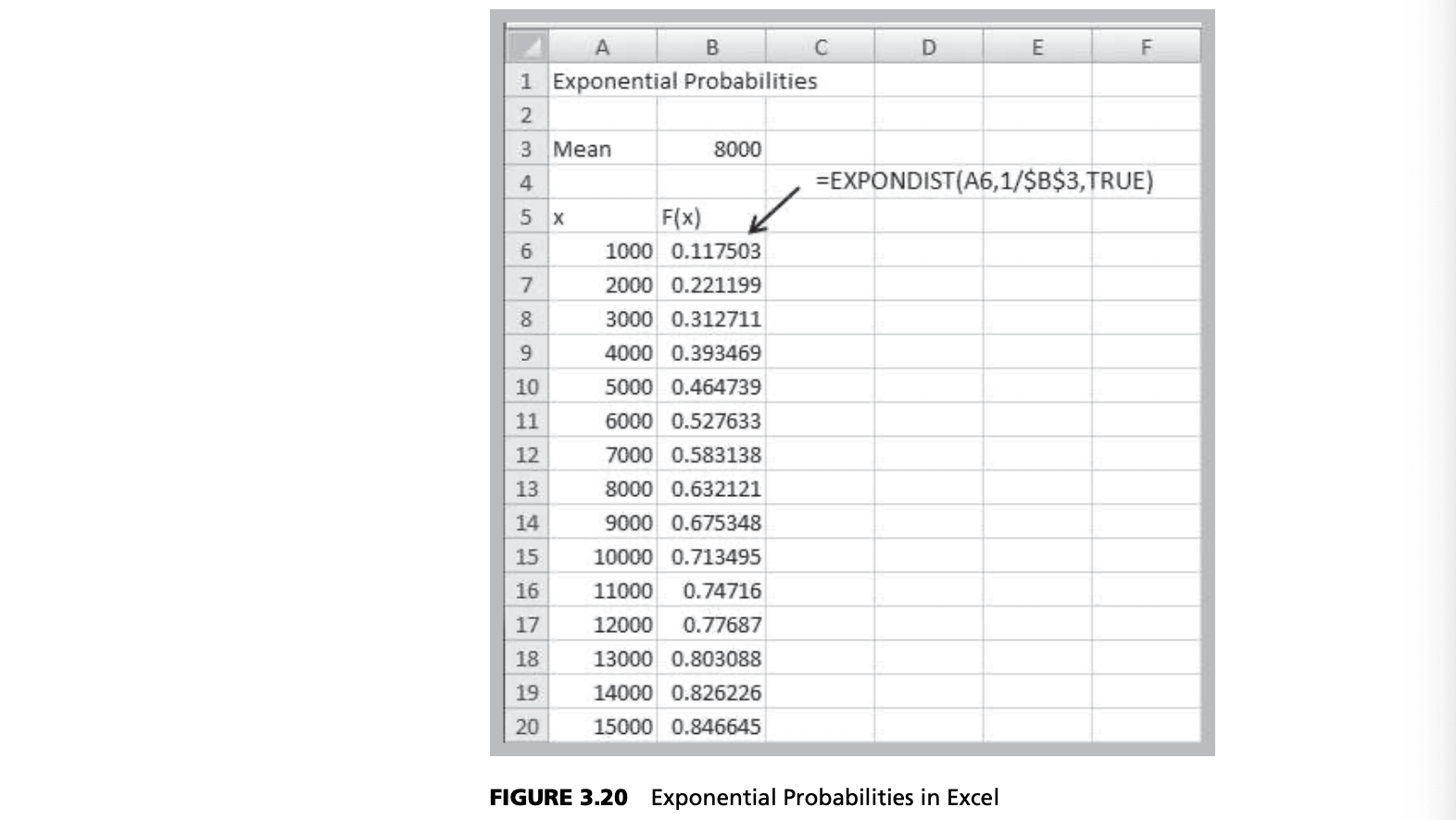
- Excel function EXPONDIST(x, lambda, cumulative).
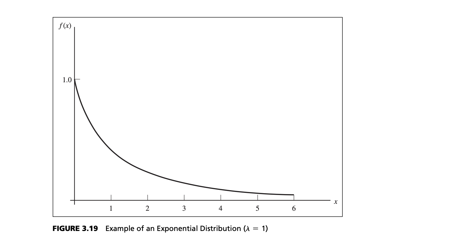
Figure 3.19 provides a sketch of the exponential distribution. The exponential distribution has the properties that it is bounded below by 0, it has its greatest density at 0, and the density declines as $x$ increases.
Example
To illustrate the exponential distribution, suppose that the mean time to failure of a critical component of an engine is $1/\lambda = 8000$ hours.
Other Useful Distributions (未完成)
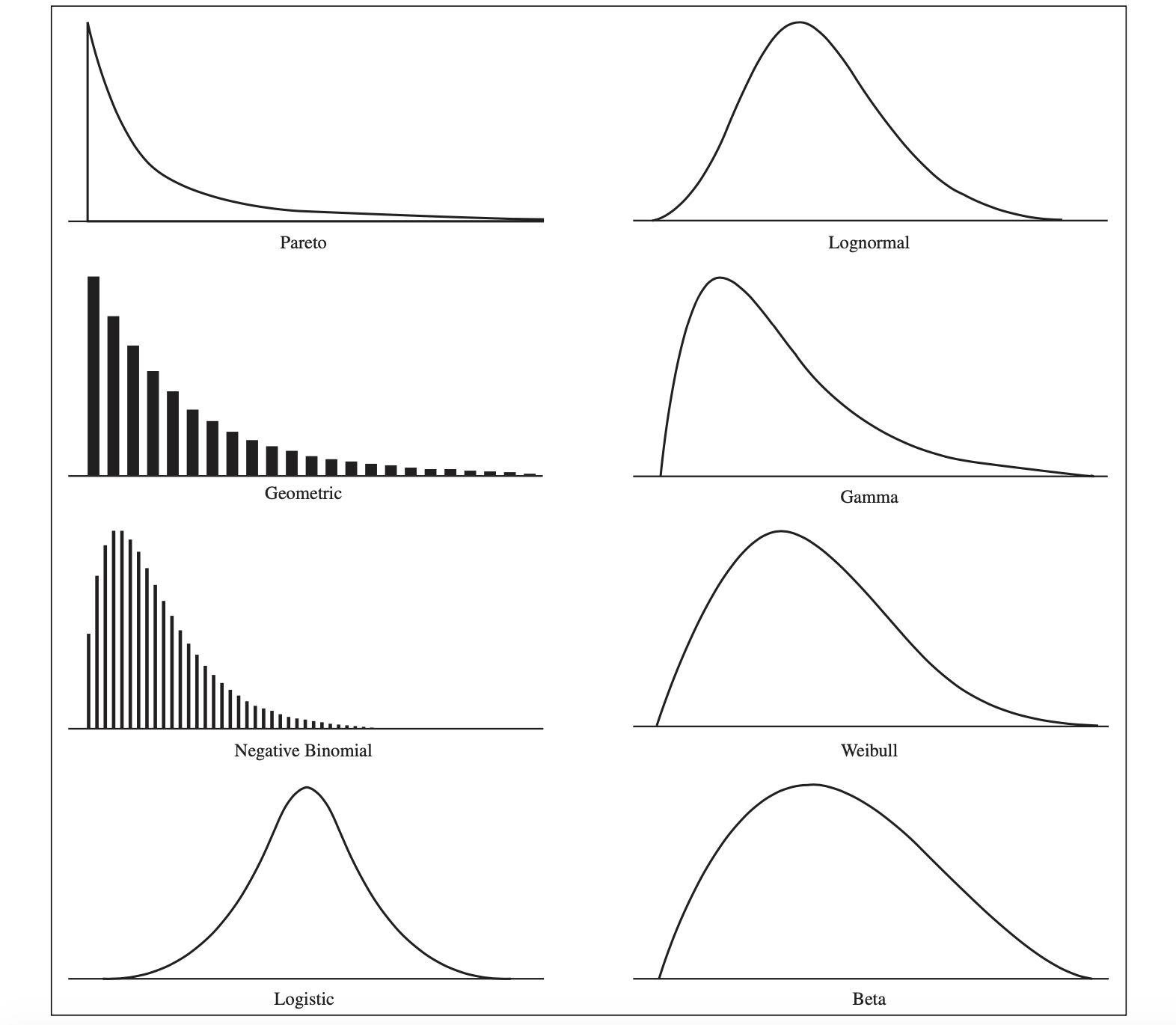
Lognormal Distribution: If the natural logarithm of a random variable $X$ is normal, then $X$ has a lognormal distribution. Because the lognormal distribution is positively skewed and bounded below by zero, it finds applications in modeling phenomena that have low probabilities of large values and cannot have negative values, such as the time to complete a task. Other common examples include stock prices and real estate prices. The lognormal distribution is also often used for “spiked” service times, that is, when the probability of 0 is very low but the most likely value is just greater than 0.
Gamma Distribution: The gamma distribution is a family of distributions defined by a shape parameter $\alpha$, a scale parameter $\beta$, and a location parameter $L$. $L$ is the lower limit of the random variable $X$; that is, the gamma distribution is defined for $X > L$. Gamma distributions are often used to model the time to complete a task, such as customer service or machine repair. It is used to measure the time between the occurrence of events when the event process is not completely random. It also finds application in inventory control and insurance risk theory.
A special case of the gamma distribution when $\alpha$ = 1 and $L = 0$ is called the Erlang distribution. The Erlang distribution can also be viewed as the sum of $k$ independent and identically distributed exponential random variables. The mean is $k/\lambda$, and the variance is $k/\lambda^2$. When $k = 1$, the Erlang is identical to the exponential distribution. For $k = 2$, the distribution is highly skewed to the right. For larger values of $k$, this skewness decreases, until for $k = 20$, the Erlang distribution looks similar to a normal distribution. One common application of the Erlang distribution is for modeling the time to complete a task when it can be broken down into independent tasks, each of which has an exponential distribution.- With a shape parameter $k$ and a scale parameter $θ$.
- With a shape parameter $α = k$ and an inverse scale parameter $β = 1/θ$, called a rate parameter.
- With a shape parameter $k$ and a mean parameter $μ = kθ = α/β$.
- For large $k$ the gamma distribution converges to normal distribution with mean $μ = kθ$ and variance $σ^2 = kθ^2$.
- $\sigma^2 = \mu \times \theta \Rightarrow \theta = \sigma^2/\mu$
- $\beta = \mu/\sigma^2$
- $\alpha = \mu \times \beta$
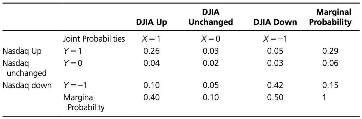
Joint and Marginal Probability Distributions
- Joint probability distribution: A probability distribution that specifies the probabilities of outcomes of two different random variables, $X$ and $Y$, that occur at the same time, or jointly
- Marginal probability: probability associated with the outcomes of each random variable regardless of the value of the other
Example
- DJIA up; NASDAQ up: 26%
- DJIA down; NASDAQ up: 5%
- DJIA unchanged; NASDAQ up: 3%
- DJIA up; NASDAQ down: 10%
- DJIA down; NASDAQ down: 42%
- DJIA unchanged; NASDAQ down: 5%
- DJIA up; NASDAQ unchanged: 4%
- DJIA down; NASDAQ unchanged: 3%
- DJIA unchanged; NASDAQ unchanged: 2%
CHAPTER 4: SAMPLING, ESTIMATION, SIMULATION
STATISTICAL SAMPLING
Need for Sampling
- Very large populations
- Destructive testing
- Continuous production process
Sample Design
- Sampling Plan – a description of the approach that will be used to obtain samples from a population
- Objectives
- The objective of a sampling study might be to estimate key parameters of a population, such as a mean, proportion, or standard deviation.
- Another application of sampling is to determine if significant differences exist between two populations.
- Target population
- Population frame: the list from which the sample is selected
- The ideal frame is a complete list of all members of the target population.
- Method of sampling
- Operational procedures for data collection
- Statistical tools for analysis
- Objectives
Sampling Methods
- Subjective
- Judgment sampling: in which expert judgment is used to select the sample (survey the “best” customers)
- Convenience sampling: in which samples are selected based on the ease with which the data can be collected (survey all customers I happen to visit this month)
- Probabilistic
- Simple Random Sampling – every subset of a given size has an equal chance of being selected
- Systematic sampling[4131] : This is a sampling plan that selects items periodically from the population.
- Stratified Sampling[4132] : This type of sampling applies to populations that are divided into natural subsets (strata) and allocates the appropriate proportion of samples to each stratum.
- Cluster sampling[4133] : This is based on dividing a population into subgroups(clusters), sampling a set of clusters, and (usually) conducting a complete census within the clusters sampled.
- Sampling from a continuous process[4134] : Selecting a sample from a continuous manufacturing process can be accomplished in two main ways.
Errors in Sampling
- Nonsampling error
- Poor sample design
- Sampling (statistical) error (although it can be minimized, it cannot be totally avoided.)
- Depends on sample size
- Tradeoff between cost of sampling and accuracy of estimates obtained by sampling
RANDOM SAMPLING FROM PROBABILITY DISTRIBUTIONS
- Random number[42] - uniformly distributed between 0 and 1
- Excel function RAND()
- Press F9 for mandatory refresh
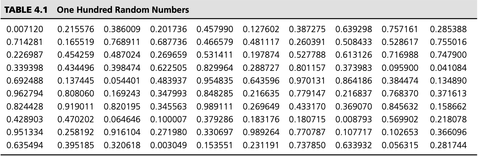
Sampling from Discrete Probability Distributions
- Rolling two dice - Combine it and the previous chart we developed a technique to roll dice on a computer.
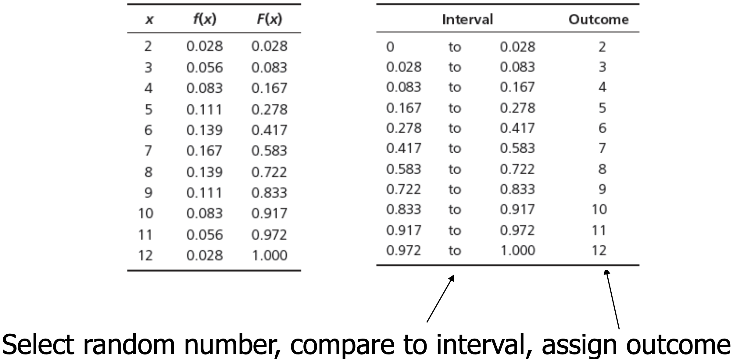
Sampling from Common Probability Distributions
- Random Variate - a value randomly generated from a specified probability distribution
- We can transform random numbers into random variates using the cumulative distribution function or special formulas
- Uniform random variate: random variate from a uniform distribution between a and b
- : $U = a + (b – a)*RAND()$
- Uniform random variate: random variate from a uniform distribution between a and b
Random Variates in Excel
- NORM.INV(RAND( ), mean, standard_deviation)
- normal distribution with a spec- ified mean and standard deviation
- NORM.S.INV(RAND( ))
- standard normal distribution
- LOGNORM.INV(*RAND( ), mean, standard_deviation)
- lognormal distribution, where ln(X) has the specified mean and standard deviation
- BETA.INV(RAND( ), alpha, beta, A, B*)
- beta distribution
- GAMMA.INV(RAND( ), alpha, beta)
- gamma distribution
A Statistical Sampling Experiment in Finance
- In finance, one way of evaluating capital budgeting projects is to compute a profitability index ($PI$), which is defined as the ratio of the present value of future cash flows (PV ) to the initial investment ($I$):
$$PI = PV/I$$
Example
- Suppose that $PV$ is estimated to be normally distributed with a mean of $12 million and a standard deviation of $2.5 million, and the initial investment is also estimated to be normal with a mean of $3.0 million and standard deviation of $0.8 million. What is the distribution of $PI$?
Solution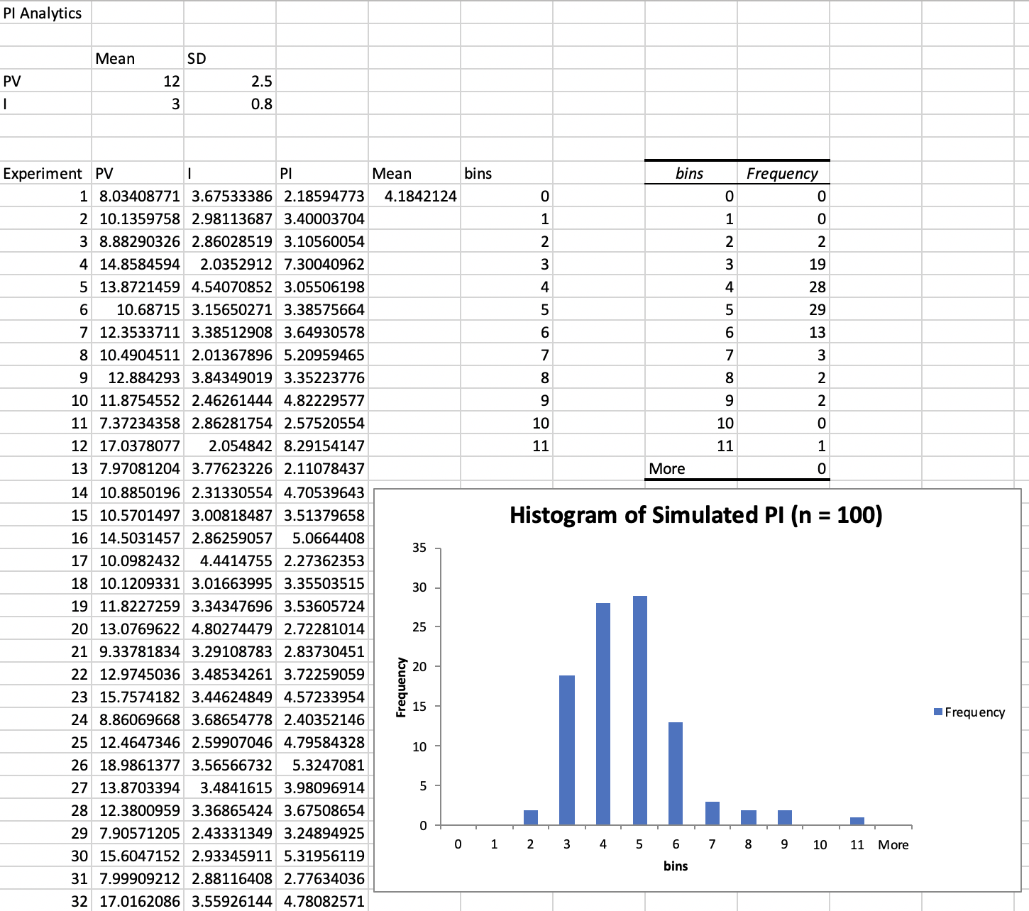
Conclusion
The ratio of two normal random variables is NOT normal!
SAMPLING DISTRIBUTIONS AND SAMPLING ERROR
- How good is an estimate of the mean obtained from a sample?
Experiment
- Assume that a random variable is uniformly distributed between 0 and 10. The expected value is $(0 + 10)/2 = 5$, the variance is $(10 – 0)^2/12 = 8.33$, and the standard deviation is 2.89.
- Generate a sample of size $n = 25$ for this random variable using the Excel function $10*RAND( )$ and compute the sample mean. Repeat this experiment several more times, say $20$, and obtain a set of $20$ sample means.
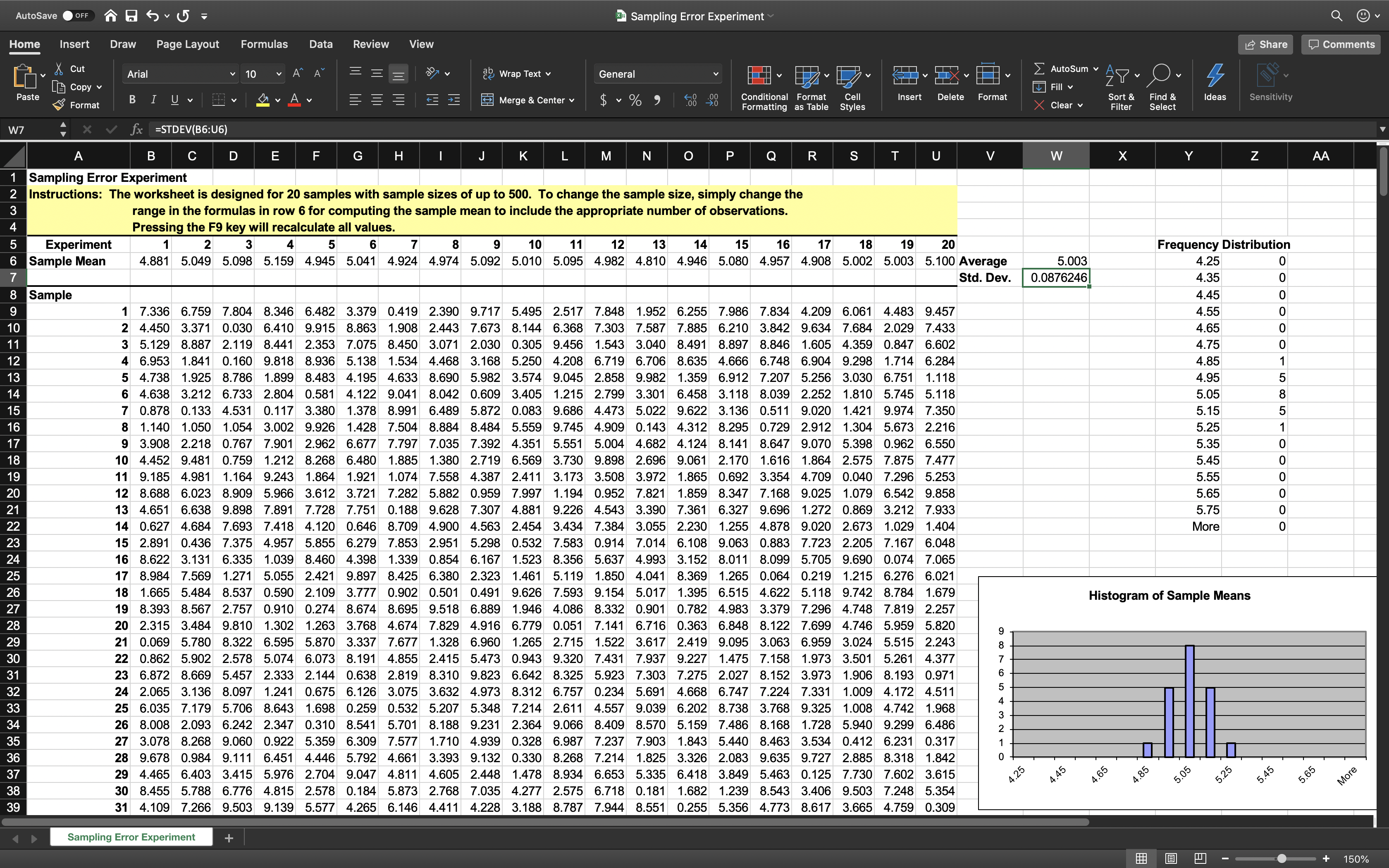
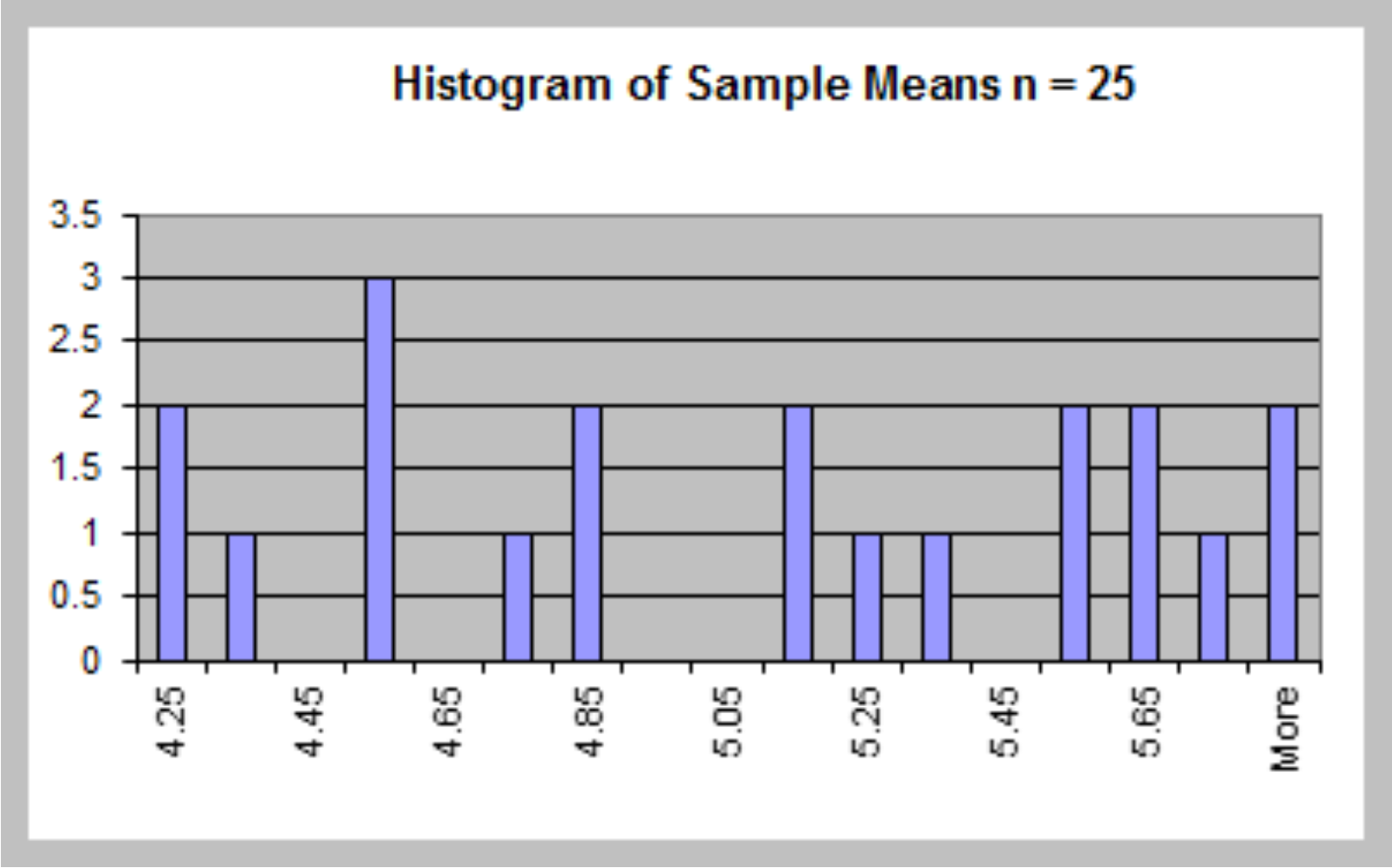
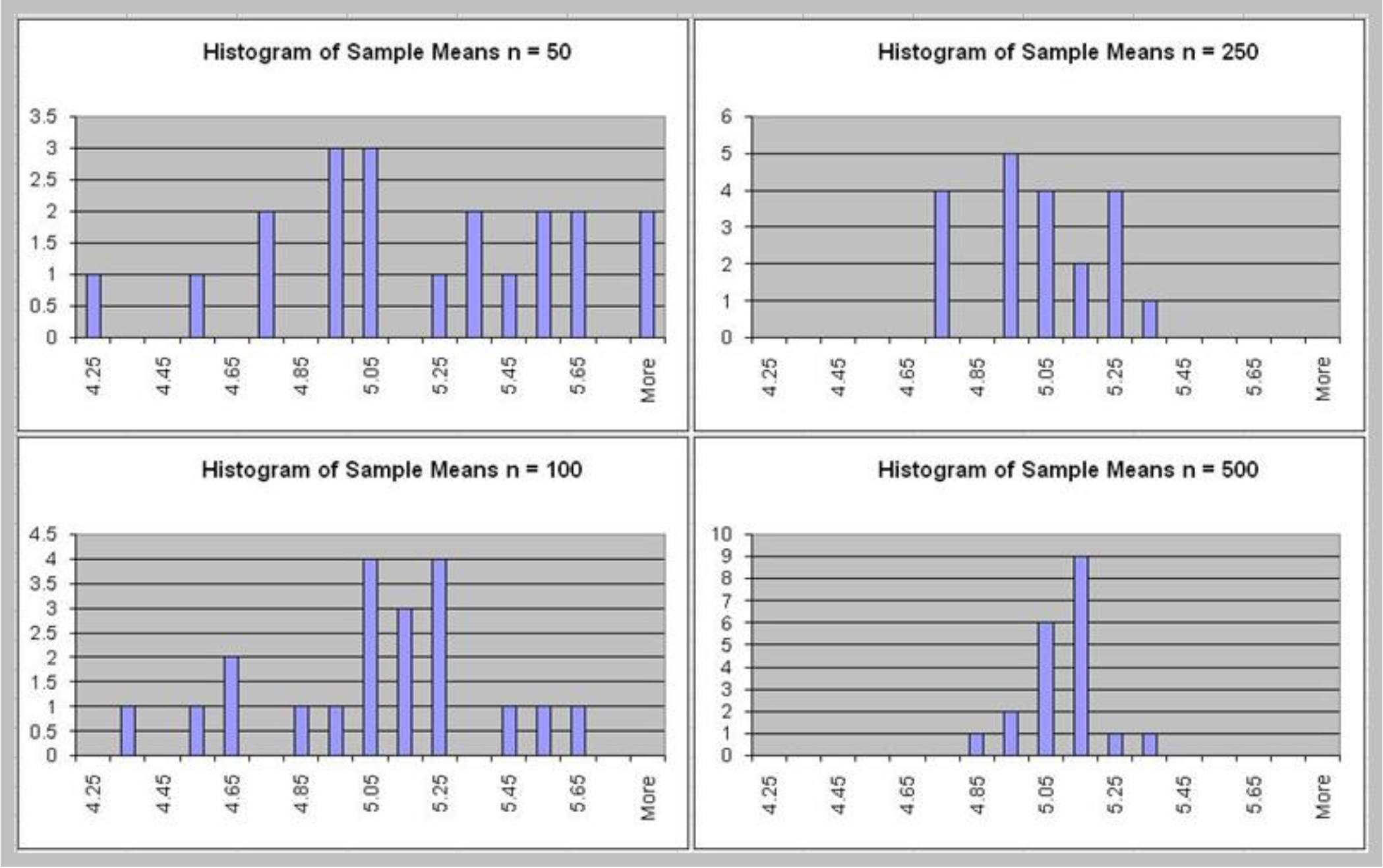
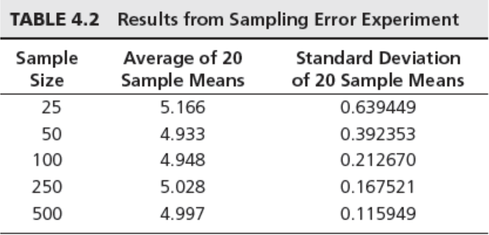
Key observations
- All means appear close to the expected value of 5.
- The standard deviation gets smaller as the sample
size increases.
Sampling Distribution of the Mean
- Sampling distribution<span class=”hint–top hint–error hint–medium hint–rounded hint–bounce” aria-label=”For example, consider a normal population with mean $\mu$ and variance $\sigma ^{2}$. Assume we repeatedly take samples of a given size from this population and calculate the arithmetic mean ${\bar x}$ for each sample – this statistic is called the sample mean. The distribution of these means, or averages, is called the “sampling distribution of the sample mean””>[431] of the mean is the distribution of the means of all possible samples of a fixed size from some population.
- Understanding sampling distributions is the key to statistical inference.
Properties of the Sampling Distribution of the Mean
- Expected value of the sample mean is the population mean, $\mu$
- Variance of the sample mean is $\sigma^2/n$, where $\sigma^2$ is the variance of the population
- Standard deviation of the sample mean, called the standard error of the mean, is $\sqrt {\sigma^2/n} = \sigma/\sqrt{n}$
Central Limit Theorem
- If the sample size is large enough (generally at least 30, but depends on the actual distribution), the sampling distribution of the mean is approximately normal, regardless of the distribution of the population.
- If the population is normal, then the sampling distribution of the mean is exactly normal for any sample size.
Applying the Sampling Distribution of the Mean - Example 1
- Suppose that the size of individual customer orders (in dollars), $X$, from a major discount book publisher Web site is normally distributed with a mean of 36 and standard deviation of 8. What is the probability that the next individual who places an order at the Web site will purchase more than 40?
$$P(X>40)=1–NORMDIST(40,36,8,TRUE)= 1 – 0.6915 = 0.3085$$
- Suppose that a sample of 16 customers is chosen. What is the probability that the mean purchase for
these 16 customers will exceed 40? - The sampling distribution of the mean will have a mean of 36, but a standard error of $8/\sqrt{16} = 2$
$$P(\bar X > 40) = 1 – NORMDIST(40,36,2,TRUE) = 1 - 0.9772 = 0.0228$$
- The calculation uses the standard deviation of the individual customer orders.
SAMPLING AND ESTIMATION
- Estimation: assessing the value of an unknown population parameter using sample data.
- Point estimate: a single number used to estimate a population parameter
- Confidence interval estimate: a range of values between which a population parameter is believed to be along with the probability that the interval correctly estimates the true population parameter
Sampling and Estimation Support in Excel
| Excel Function | Description |
|---|---|
| CONFIDENCE.NORM(alpha, standard_dev, size) | Returns the confidence interval for a population mean using a normal distribution |
| CONFIDENCE.T(alpha, standard_dev, size) | Returns the confidence interval for a population mean using a t‐distribution |
| T.INV(probability, deg_freedom) | Returns the left‐tailed inverse of the t‐distribution |
| CHISQ.DIST(x, deg_freedom) | Returns the probability above $x$ for a given value of degrees of freedom. |
| CHISQ.INV(probability, deg_freedom) | Returns the value of x that has a right‐tail area equal to probability for a specified degree of freedom. |
| Analysis Toolpak Tools | Description |
|---|---|
| SAMPLING | Creates a simple random sample with replacement or a systematic sample from a population |
| Analysis Toolpak Tools | Description |
|---|---|
| Random Sample Generator | Generates a random sample without replacement |
| Confidence Intervals | Computes confidence intervals for means with $\sigma$ known or unknown, proportions, and population total |
| Sample Size | Determines sample sizes for means and proportions |
Point Estimates
- Notice that there are some considerable differences as compared to the population parameters because of sampling error.
- A point estimate alone does not provide any indication of the magnitude of the potential error in the estimate.
| Common Point Estimate | Population Parameter |
|---|---|
| Sample mean, $\bar x$ | Population mean, $\mu$ |
| Sample variance, $s^2$ | Population variance, $\sigma ^2$ |
| Sample standard deviation, $s$ | Population standard deviation, $\sigma$ |
| Sample proportion, $\hat p$ | Population proportion, $\pi$ |
Example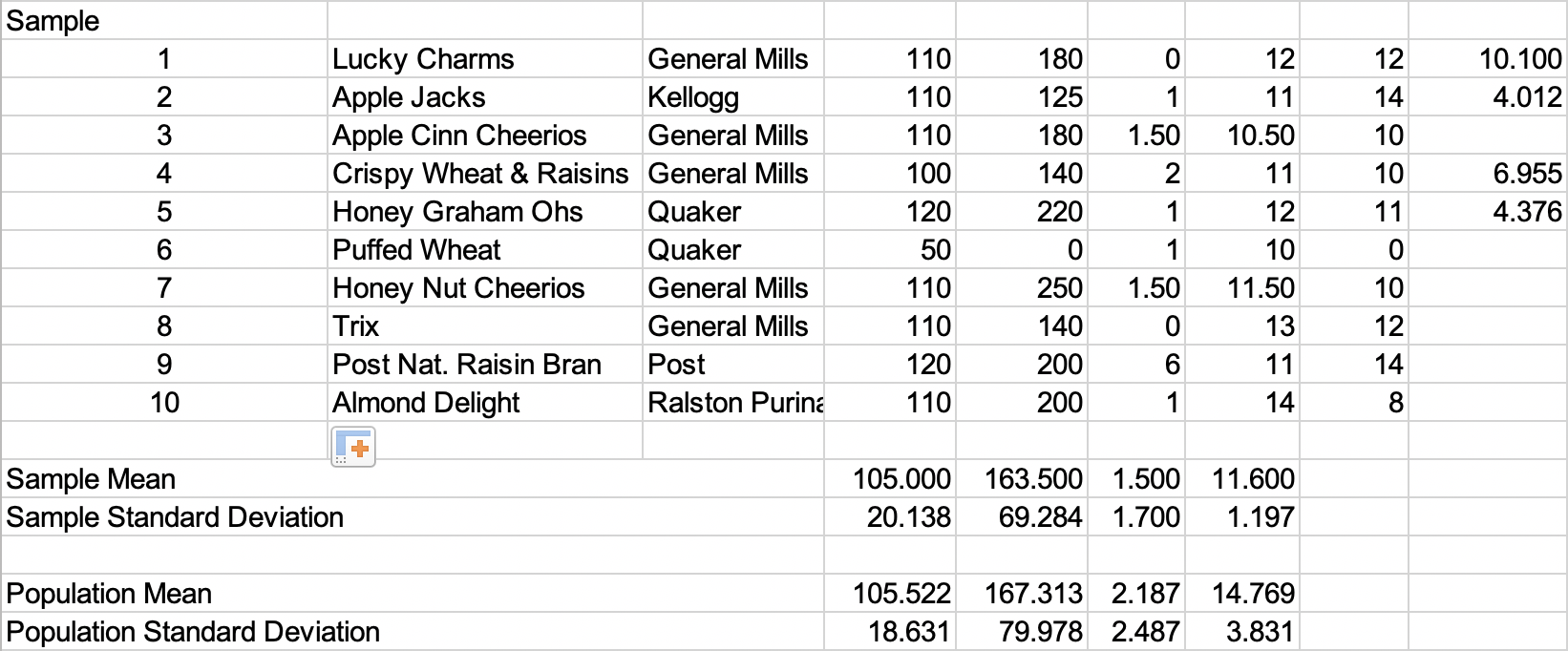
Unbiased Estimators
Unbiased estimator – one for which the expected value equals the population parameter it is intended to estimate
The sample variance is an unbiased estimator for the population variance
$$\displaystyle \sigma^2 = \frac{\sum ^{n}_{i=1}{(x_i - \mu)}^2}{N}$$
$$\displaystyle s^2 = \frac{\sum ^{n}_{i=1}{(x_i - \bar x)}^2}{n-1}$$
It seems quite intuitive that the sample mean should provide a good point estimate for the population mean. However, it may not be clear why the formula for the sample variance $s^2$, which has a denominator of $n - 1$, particularly because it is different from the formula for the population variance.
Why is this so? Statisticians develop many types of estimators, and from a theoretical as well as a practical perspective, it is important that they “truly estimate” the population parameters they are supposed to estimate. Suppose that we perform an experiment in which we repeatedly sampled from a population and computed a point estimate for a population parameter. Each individual point estimate will vary from the population parameter; however, we would hope that the long‐term average (expected value) of all possible point estimates would equal the population parameter. If the expected value of an estimator equals the population parameter it is intended to estimate, the estimator is said to be unbiased. If this is not true, the estimator is called biased and will not provide correct results.
Fortunately, all the estimators in Common Point Estimates are unbiased and, therefore, are meaning-ful for making decisions involving the population parameter. In particular, statisticians have shown that the denominator $n - 1$ used in computing $s^2$ is necessary to provide an unbiased estimator of $\sigma^2$ . If we simply divide by the number of observations, the estimator would tend to underestimate the true variance.
Interval Estimates
- Range within which we believe the true population parameter falls
- Example: Gallup poll – percentage of voters favoring a candidate is 56% with a 3% margin of error.
- Interval estimate is [53%, 59%]
- A $100 \times (1 – a)%$ probability interval is any interval $[A, B]$ such that the probability of falling between $A$ and $B$ is $1 – a$
Confidence Intervals: Concepts and Applications
- Confidence interval (CI): an interval estimated that specifies the likelihood that the interval contains the true population parameter
- Level of confidence $(1 – a)$: the likelihood that the CI contains the true population parameter, usually expressed as a percentage (90%, 95%, 99% are most common).
The margin of error depends on the level of confidence and the sample size. For example, suppose that the margin of error for some sample size and a level of confidence of 95% is calculated to be 2.0. One sample might yield a point estimate of 10. Then a 95% confidence interval would be [8, 12]. However, this interval may or may not include the true population mean. If we take a different sample, we will most likely have a different point estimate, say 10.4, which, given the same margin of error, would yield the interval estimate [8.4, 12.4]. Again, this may or may not include the true population mean. If we chose 100 differ- ent samples, leading to 100 different interval estimates, we would expect that 95% of them—the level of confidence—would contain the true population mean. We would say we are “95% confident” that the interval we obtain from sample data contains the true population mean. The higher the confidence level, the more assurance we have that the interval contains the true population parameter. As the confidence level increases, the confidence interval becomes larger to provide higher levels of assurance. You can view $a$ as the risk of incorrectly concluding that the confidence interval contains the true mean.
When national surveys or political polls report an interval estimate, they are actually confidence intervals. However, the level of confidence is generally not stated because the average person would probably not understand the concept or terminology. While not stated, you can probably assume that the level of confidence is 95%, as this is the most common value used in practice.
Confidence Interval for the Mean - $\sigma$ Known
The simplest type of confidence interval is for the mean of a population where the standard deviation is assumed to be known. You should realize, however, that in nearly all practical sampling applications, the population standard deviation will not be known. However, in some applications, such as measurements of parts from an automated machine, a process might have a very stable variance that has been established over a long history, and it can reasonably be assumed that the standard deviation is known.
In most practical applications, samples are drawn from very large populations. If the population is relatively small compared to the sample size, a modification must be made to the confidence interval. Specifically, when the sample size, n, is larger than 5% of the population size, N, a correction factor is needed in computing the margin of error.
To fully understand these results, it is necessary to examine the formula used to compute the confidence interval. A $100(1 - a)$%, confidence interval for the population mean $\mu$ is given by:
$\bar x \pm Z_{a/2}(\sigma/\sqrt{n})$
Note that this formula is simply the sample mean, point estimate, plus or minus a margin of error. The margin of error is a number $Z_{a/2}$ times the standard error of the sampling distribution of the mean, $\sigma/\sqrt{n}$. The value represents the value of a standard normal random variable that has a cumulative probability of $a/2$, which could be computed in Excel using the function NORM.S.INV ($a/2$).
Sampling From Finite Populations
- FPC(Finite Populations Correlation) factor: $\displaystyle \sqrt{\frac{N - n}{N - 1}}$
- When $n > 5% \space N$, use a correction factor in computing the standard error:
- $\displaystyle \frac{\sigma}{\sqrt{n}} \sqrt{\frac{N - n}{N - 1}}$
Key Observation
- As the confidence level $(1 - a)$ increases, the width of the confidence interval also increases.
- As the sample size increases, the width of the confidence interval decreases.
Confidence Interval for the Mean - $\sigma$ Unknown
In most practical applications, the standard deviation of the population is unknown, and we need to calculate the confidence interval differently.
Instead of using $\Z_{a/2}$ based on the normal distribution, the tool uses a “t‐value” with which to multiply the standard error to compute the interval half‐width. The t‐value comes from a new probability distribution called the t‐distribution. The t‐distribution is actually a family of probability distributions with a shape similar to the standard normal distribution. Different t‐distributions are distinguished by an additional parameter, degrees of freedom (df ).
The concept of “degrees of freedom” can be puzzling. It can best be explained by examining the formula for the sample variance:
$$\displaystyle s^2 = \frac{\sum^{n}_{i=1}(x_i - \bar x)^2}{n-1}$$
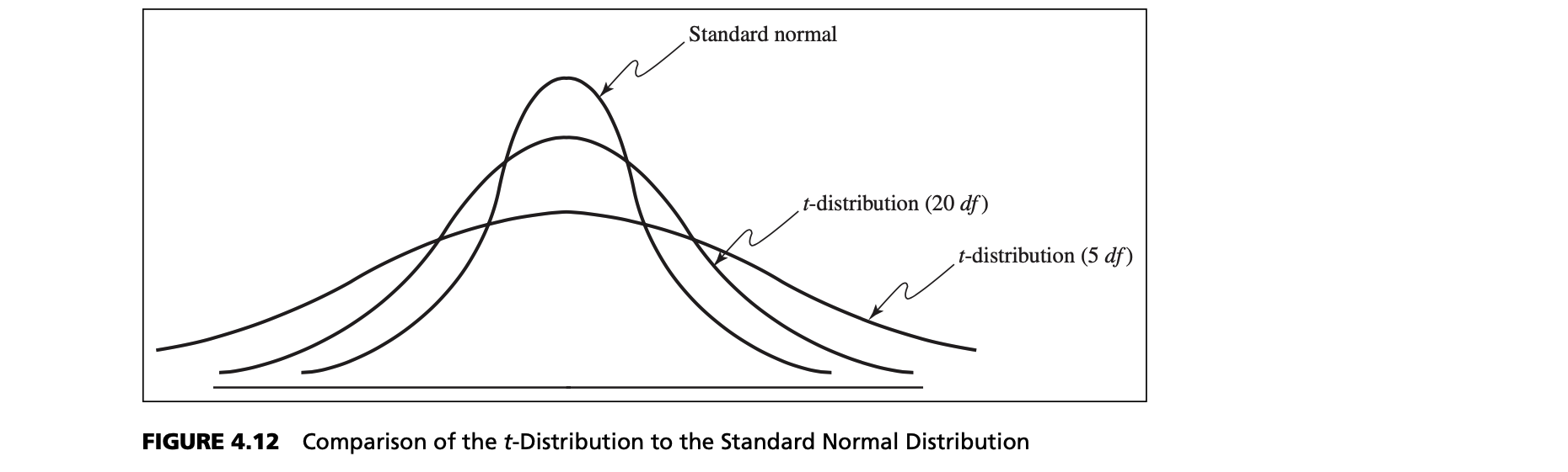
Relationship Between Normal Distribution and t-distribution
The t‐distribution has a larger variance than the standard normal, thus making confidence intervals wider than those obtained from the standard normal distribution, in essence correcting for the uncertainty about the true standard deviation. As the number of degrees of freedom increases, the t‐distribution converges to the standard normal distribution.
t-distribution
The number of sample values that are free to vary defines the number of degrees of freedom; in general, df equals the number of sample values minus the number of estimated parameters. Because the sample variance uses one estimated parameter, the mean, the t‐distribution used in confidence interval calculations has $n - 1$ degrees of freedom. Because the t‐distribution explicitly accounts for the effect of the sample size in estimating the population variance, it is the proper one to use for any sample size. However, for large samples, the difference between t‐ and z‐values is very small, as we noted earlier.
The formula for a $100(1 - a)%$, confidence interval for the mean m when the population standard deviation is unknown is:
$\bar x \pm t_{a/2, n-1}(s/\sqrt n)$
$t_{a/2, n-1}$ is the value from the t‐distribution with $n - 1$ degrees of freedom, giving an upper‐tail probability of $a/2$.
- using the Excel function T.INV(1‐ $a/2$, $n - 1$).
Confidence Interval for the Proportion
For categorical variables having only two possible outcomes, such as good or bad, male or female, and so on, we are usually interested in the proportion of observations in a sample that has a certain characteristic. An unbiased estimator of a population proportion $\pi$ is the statistic $\hat p = x/n$ (the sample proportion), where $x$ is the number in the sample having the desired characteristic and $n$ is the sample size.
Sample Proportion
- Sample proportion: $\hat p= x/n$
- x = number in sample having desired
characteristic - n = sample size
- x = number in sample having desired
- The sampling distribution of $\hat p$ has mean $\pi$ and variance $\pi(1-\pi)/n$
- When $n\pi$ and $n(1 – \pi)$ are at least 5, the sampling distribution of p approach a normal distribution
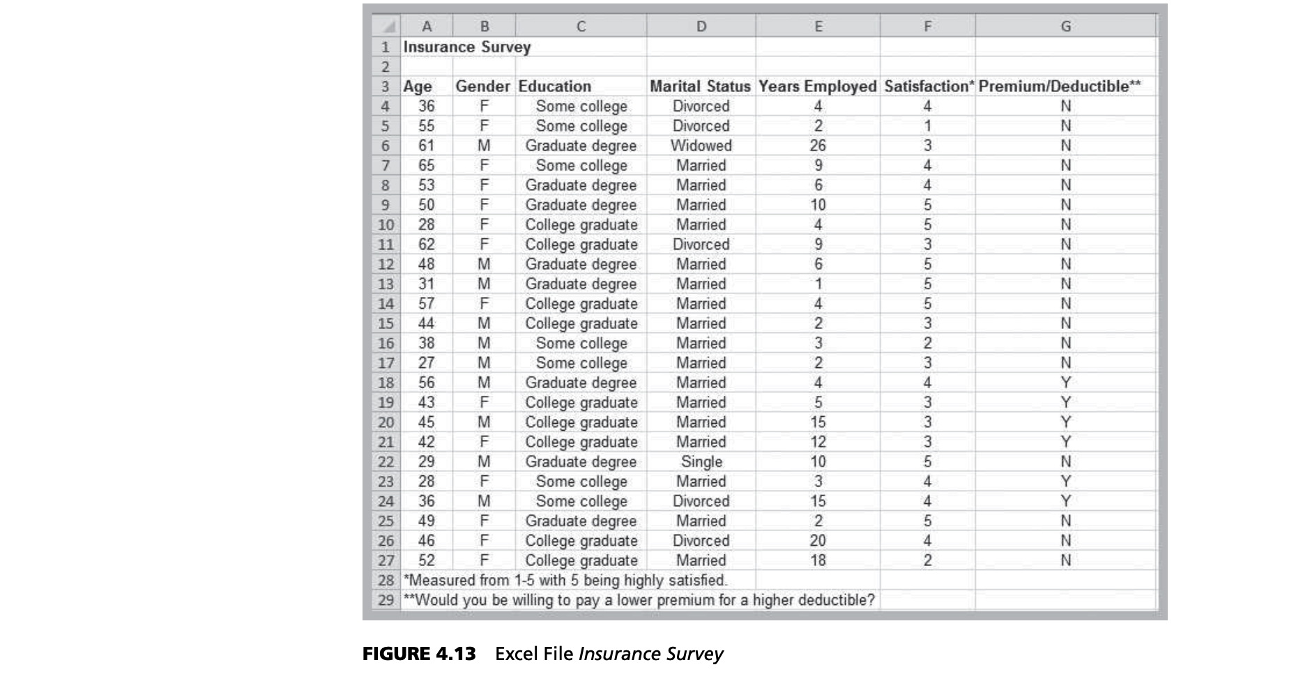
Example
The Excel sheet describes whether a sample of employees would be willing to pay a lower premium for a higher deductible for their health insurance. Suppose we are interested in the proportion of individuals who answered yes. We may easily confirm that 6 out of the 24 employees, or 25%, answered yes. Thus, a point estimate for the proportion answering yes is $\hat p = 0.25$.
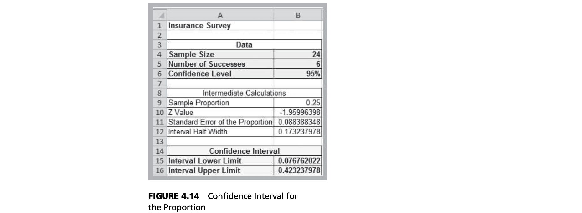
Notice that this is a fairly large confidence interval, suggesting that we have quite a bit of uncertainty as to the true value of the population proportion. This is because of the relatively small sample size.
These calculations are based on the following: a 100(1 - a) confidence interval for the proportion is:
$\hat p \pm Z_{a/2} \sqrt {\frac{\hat p (1 - \hat p)}{n}}$
Notice that as with the mean, the confidence interval is the point estimate plus or minus some margin of error. In this case, $\sqrt {(\hat p(1 - \hat p)/n}$ is the standard error for the sampling distribution of the proportion.
Confidence Intervals for the Variance and Standard Deviation
Understanding variability is critical to effective decisions. Thus, in many situations, one is interested in obtaining point and interval estimates for the variance or standard deviation.
Calculation of the confidence intervals for variance and standard deviation is quite different from the other confidence intervals we have studied. Although we use the sample standard deviation $s$ as a point estimate for $\sigma$, the sampling distribution of $s$ is not normal, but is related to a special distribution called the chi-square ($\chi^2$) distribution. The chi‐square distribution is characterized by degrees of freedom, similar to the t‐distribution.
However, unlike the normal or t‐distributions, the chi‐square distribution is not symmetric, which means that the confidence interval is not simply a point estimate plus or minus some number of standard errors. The point estimate is always closer to the left endpoint of the interval. A $100(1 - a)%$, confidence interval for the
variance is:
$$[\frac{(n-1)s^2}{\chi ^2_{n-1, a/2}}, \frac{(n-1)s^2}{\chi ^2_{n-1, 1-a/2}}]$$
Sampling Distribution of $s$
- The sample standard deviation, $s$, is a point estimate for the population standard deviation, $\sigma$
- The sampling distribution of $s$ has a chi-square ($\chi^2$) distribution with $n-1$ df
- CHISQ.DIST(x, deg_freedom) returns probability
to the right of $x$ - CHISQ.INV(probability, deg_freedom) returns the value of $x$ for a specified right-tail probability
Confidence Interval for a Population Total
In some applications, we might be more interested in estimating the total of a population rather than the mean.
For instance, an auditor might wish to estimate the total amount of receivables by sampling a small number of accounts. If a population of $N$ items has a mean $\mu$, then the population total is $N\mu$. We may estimate a population total from a random sample of size $n$ from a population of size $N$ by the point estimate $N\bar x$.
$\displaystyle N\bar x \pm t_{a/2, n-1}N\frac{s}{\sqrt n}\sqrt{\frac{N-n}{N-1}}$
Example
Suppose that an auditor in a medical office wishes to estimate the total amount of unpaid reimbursement claims for 180 accounts over 60 days old. A sample of 20 from this population yielded a mean amount of unpaid claims of 185 and the sample standard deviation is 22.
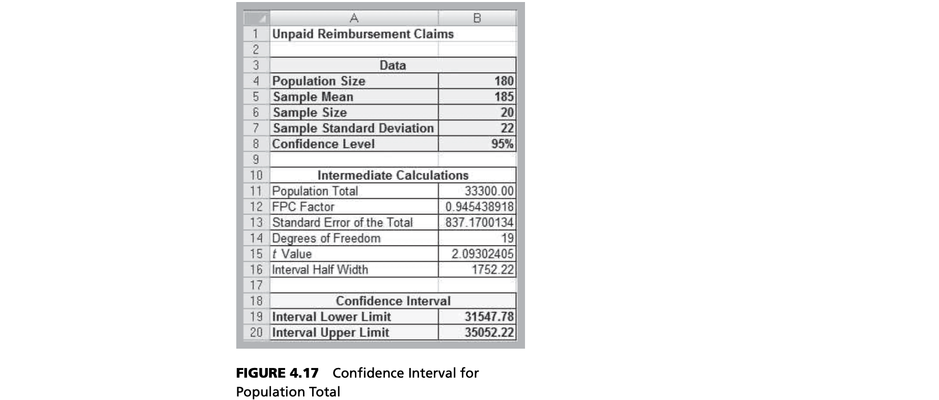
If you examine this closely, it is almost identical to the formula used for the confidence interval for a mean with an unknown population standard deviation and a finite population correction factor, except that both the point estimate and the interval half‐width are multiplied by the population size N to scale the result to a total, rather than an average.
Confidence Intervals and Decision Making
Confidence intervals can be used in many ways to support business decisions. For example, in packaging some commodity product such as laundry soap, the manufacturer must ensure that the packages contain the stated amount to meet government regulations. However, variation may occur in the filling equipment. Suppose that the required weight for one product is 64 ounces. A sample of 30 boxes is measured and the sample mean is calculated to be 63.82 with a standard deviation of 1.05. Does this indicate that the equipment is under-filling the boxes? Not necessarily. A 95% confidence interval for the mean is [63.43, 64.21]. Although the sample mean is less than 64, the sample does not provide sufficient evidence to draw that conclusion that the population mean is less than 64 because 64 is contained within the confidence interval. In fact, it is just as plausible that the population mean is 64.1 or 64.2. However, suppose that the sample standard deviation was only 0.46. The confidence interval for the mean would be [63.65, 63.99]. In this case, we would conclude that it is highly unlikely that the population mean is 64 ounces because the confidence interval falls completely below 64; the manufacturer should check and adjust the equipment to meet the standard.
As another example, suppose that an exit poll of 1,300 voters found that 692 voted for a particular candidate in a two‐person race. This represents a proportion of 53.23% of the sample. Could we conclude that the candidate will likely win the election? A 95% confidence interval for the proportion is [0.505, 0.559]. This suggests that the population proportion of voters who favor this candidate will be larger than 50%, so it is safe to predict the winner. On the other hand, suppose that only 670 of the 1,300 voters voted for the candidate, indicating a sample proportion of 0.515. The confidence interval for the population proportion is [0.488, 0.543]. Even though the sample proportion is larger than 50%, the sampling error is large, and the confidence interval suggests that it is reasonably likely that the true population proportion will be less than 50%, so it would not be wise to predict the winner based on this information.
We also point out that confidence intervals are most appropriate for cross‐ sectional data. For time‐series data, confidence intervals often make little sense because the mean and/or variance of such data typically change over time. However, for the case in which time‐series data are stationary—that is, they exhibit a constant mean and constant variance—then confidence intervals can make sense. A simple way of deter- mining whether time‐series data are stationary is to plot them on a line chart. If the data do not show any trends or patterns and the variation remains relatively constant over time, then it is reasonable to assume the data are stationary. However, you should be cautious when attempting to develop confidence intervals for time‐series data because high correlation between successive observations (called autocorrelation) can result in misleading confidence interval results.
Confidence Intervals and Sample Size
- An important question in sampling is the size of the sample to take. Note that in all the formulas for confidence intervals, the sample size plays a critical role in determining the width of the confidence interval.
- CI for the mean, $\sigma$ known
- Sample size needed for half-width of at
most E is $n \ge (Z_{a/2})^2(\sigma^2)/E^2$
- Sample size needed for half-width of at
- CI for a proportion
- Sample size needed for half-width of at most E is $n \ge \frac{(Z_{a/2}^2\pi (1 - \pi))}{E^2}$
- Use the sample proportion as an estimate of $\pi$, or 0.5 for the most conservative estimate
Prediction Intervals
- A prediction interval is one that provides a range for predicting the value of a new observation from the same population.
- A confidence interval is associated with the sampling distribution of a statistic, but a prediction interval is associated with the distribution of the random variable itself.
- A 100(1 – a)% prediction interval for a new observation is
- $\bar x \pm t_{a/2, n-1}(s \sqrt {1+1/n}$
Additional Additional Types of Confidence Intervals
Sampling Distribution of the Mean – Theory
Interval Estimate Containing the True Population Mean
Interval Estimate Not Containing the True Population Mean
CI for Difference in Means
Independent Samples with Unequal Variances
Independent Samples with Equal Variances
Paired Samples
Differences Between Proportions
Summary of CI Formulas
| Type of Confidence Interval | Formula |
|---|---|
| Mean, SD known | $\displaystyle \bar x \pm Z_{a/2}(a/\sqrt{n})$ |
| Mean, SD unknown | $\displaystyle \bar x \pm t_{a/2, n-1}(s/\sqrt{n})$ |
| Proportion | $\displaystyle \hat p \pm Z_{a/2} \sqrt{\frac{\hat p(1-\hat p)}{n}}$ |
| Population total | $\displaystyle N\bar x \pm ($ |
| Difference between means, independent sample | |
| Variance | $$\displaystyle [\frac{(n-1)s^2}{\chi ^2_{n-1, a/2}},\frac{(n-1)s^2}{\chi ^2_{n-1, 1-a/2}}]$$ |
CHAPTER 6: REGRESSION ANALYSIS
Regression analysis
- Building models that characterize the relationships between a dependent variable and one (single) or more (multiple) independent variables, all of which are numerical.
- simple regression: single independent variable
- Multiple regression: two or more independent variables.
- Regression analysis can be used for:
- Cross-sectional data
- Time series data (forecasting)
Example – Multiple Regression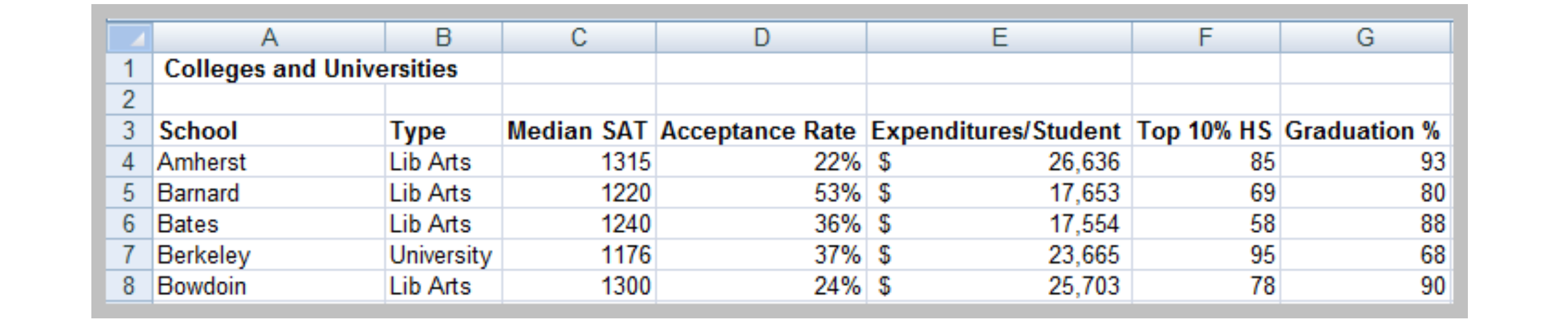
As another example, many colleges try to predict students’ performance as a function of several characteristics. We might wish to predict the graduation rate as a function of the other variables—median SAT, acceptance rate, expenditures/student, and the top 10% of their high school class. We might use the following
equation:
$$Graduation% = a + b * Median \space SAT + c * Acceptance \space Rate + d * Expenditures/Student + e * Top 10 \space % \space HS$$
Simple Linear Regression
- Single independent variable
- Linear relationship
- Variables:
- $X$: one independent variable
- $Y$: one dependent variable
- Simple linear regression model: $Y = \beta_0 + \beta_1X + \epsilon$
- $Y$: expected value
- $\beta_0 \space and \space \beta1$: population parameters that represent the intercept and slope
- $\epsilon$: for a specific value of $X$, we have many possible values of $Y$ that vary around the mean. To account for this, we add an error term to the mean
Example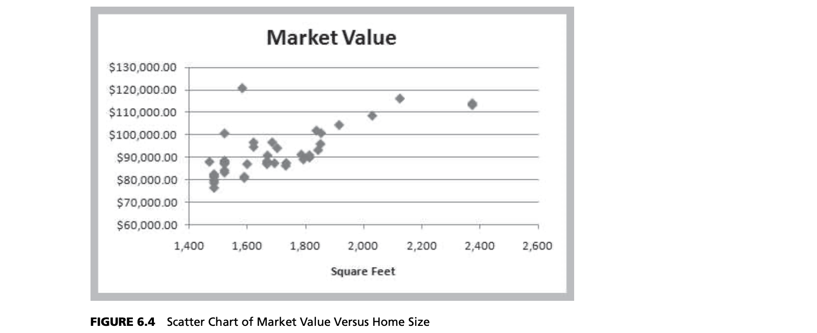
Because we don’t know the entire population, we don’t know the true values of $\beta_0$ and $\beta_1$. In practice, we must estimate these as best as we can from the sample data. Using the Home Market Value data, note that each point in Figure 6.4 represents a paired observation of the square footage of the house and its market value. If we draw a straight line through the data, some of the points will fall above the line, some below it, and a few might fall on the line itself.
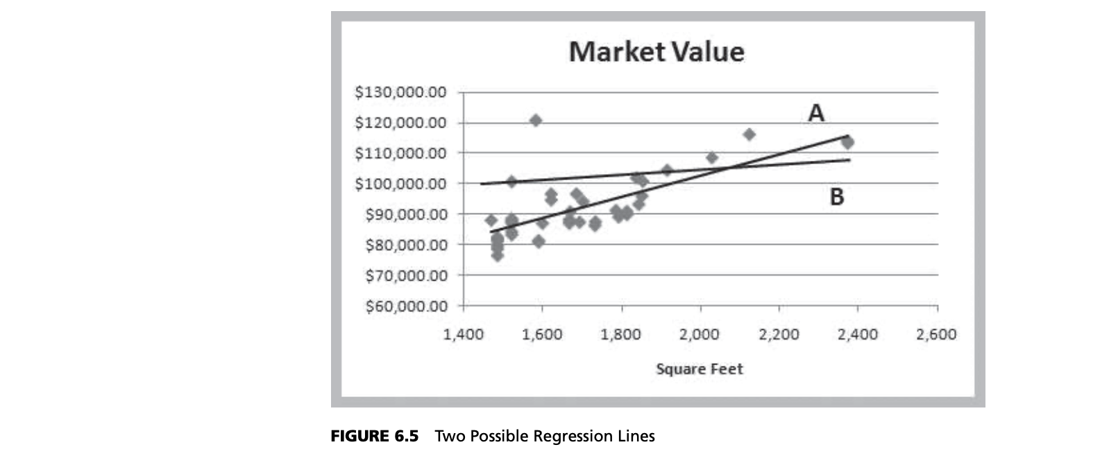
Figure 6.5 shows two possible straight lines to represent the relationship between $X$ and $Y$. Clearly, you would choose A as the better fitting line over B because all the points are “closer” to the line and the line appears to be in the “middle” of the data. The only difference between the lines is the value of the slope and intercept; thus, we seek to determine the values of the slope and intercept that provide the best‐fitting line. We do this using a technique called least‐squares regression.
Steps
- Create a scatter chart first
- Observe the scatter and judge it if it is a simple linear regression
Example – Simple Regression
For example, the market value of a house is typically related to its size.
$$Market \space Value = a + b \times Square \space Feet$$
The independent variable, $X$, is the number of square feet, and the dependent variable, $Y$, is the market value. In general, we see that higher market values are associated with larger home sizes.
Least‐Squares Regression
- Simple linear regression model:
- $Y = \beta_0 + \beta_1X + \epsilon$
- $Y$: expected value
- $\beta_0 \space and \space \beta1$: population parameters that represent the intercept and slope
- $\epsilon$: for a specific value of $X$, we have many possible values of $Y$ that vary around the mean. To account for this, we add an error term to the mean
- $Y = \beta_0 + \beta_1X + \epsilon$
- Least-squares regression estimates $\beta_0$ and $\beta_1$ by $b_0$ and $b_1$ by minimizing the sum of squares of the residuals:
- $\hat Y =b_0 + b_1X$
- $(X_i, Y_i)$: the $i$th observation
- $\hat Y$: the estimated value
- $\hat Y =b_0 + b_1X$
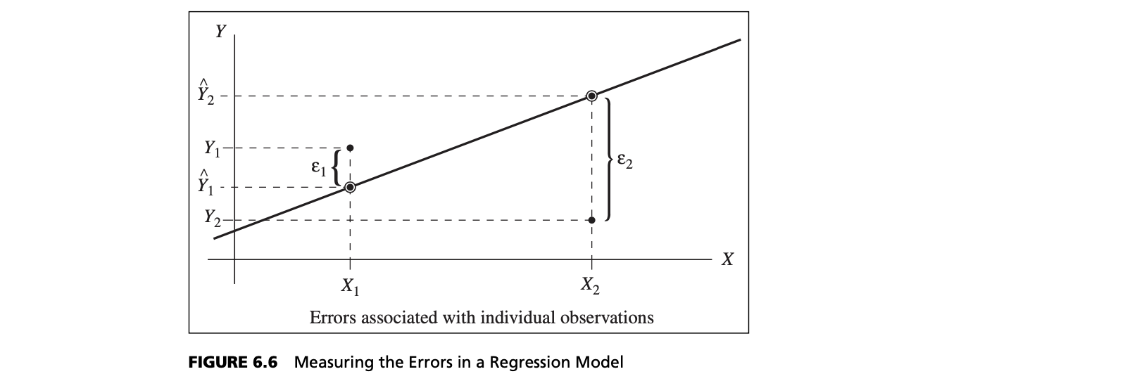
Errors(Residuals)
One way to quantify the relationship between each point and the estimated regression equation is to measure the vertical distance between them, $Y_i - \hat Y_i$(see Figure 6.6). We can think of these differences as the observed errors (often called residuals), $e_i$, associated with estimating the value of the dependent variable using the regression line. The best‐fitting line should minimize some measure of these errors. Because some errors will be negative and others positive, we might take their absolute value, or simply square them. Mathematically, it is easier to work with the squares of the errors.
Adding the squares of the errors, we obtain the following function:
$$\displaystyle \sum_{i=1}^{n}{e_i^2} = \sum_{i=1}^{n}(Y_i - \hat Y_i)^2$$
If we can find the best values of the slope and intercept that minimizes the sum of squares (hence the name, “least squares”) of the observed errors, $e_i$, we will have found the best‐fitting regression line. Note that $X_i$ and $Y_i$ are the known data and that $b_0$ and $b_1$ are unknowns in equation $\hat Y =b_0 + b_1X$. Using calculus, we can show that the solution that minimizes the sum of squares of the observed errors is:
$$\displaystyle b_i = \frac{\sum ^{n}{i=1}{X_i Y_i} - n\bar X \bar Y}{\sum ^{n}{i=1}{X_i^2 - n \bar X}}$$
$$\displaystyle b_0 = \bar Y - b_1 \bar X$$
Excel
| Functions | Description |
|---|---|
| Excel Function | |
| INTERCEPT(known_y’s, known_x’s) | Calculates the intercept for a least‐squares regression line |
| SLOPE(known_y’s, known_x’s) | Calculates the slope of a linear regression line |
| TREND(known_y’s, known_x’s, new_x’s) | Computes the value on a linear regression line for specified values of the independent variable |
| Analysis Toolpak Tools | |
| Regression | Performs linear regression using least squares |
| PHStat Add‐In | |
| Simple Linear Regression | Generates a simple linear regression analysis |
| Multiple Regression | Generates a multiple linear regression analysis |
| Best Subsets | Generates a best‐subsets regression analysis |
| Stepwise Regression | Generates a stepwise regression analysis |
Skill‐Builder Exercise 6.2 202
A Practical Application of Simple Regression to Investment Risk 202
Simple Linear Regression in Excel 203
Skill‐Builder Exercise 6.3 204
Regression Statistics 204
Regression as Analysis of Variance 205
Testing Hypotheses for Regression Coefficients 205 Confidence Intervals for Regression Coefficients 206 Confidence and Prediction Intervals for X‐Values 206
Residual Analysis and Regression Assumptions 206 Standard Residuals 208
Skill‐Builder Exercise 6.4 208
Checking Assumptions 208
Multiple Linear Regression 210
Skill‐Builder Exercise 6.5 210
Interpreting Results from Multiple Linear Regression 212
Correlation and Multicollinearity 212 Building Good Regression Models 214
Stepwise Regression 217
Skill‐Builder Exercise 6.6 217
Best‐Subsets Regression 217
The Art of Model Building in Regression 218 Regression with Categorical Independent Variables
Categorical Variables with More Than Two Levels 223
Skill‐Builder Exercise 6.7 225
Regression Models with Nonlinear Terms 225
Skill‐Builder Exercise 6.8 226
Basic Concepts Review Questions 228 Problems and Applications 228
Case: Hatco 231
CHAPTER 7 FORECASTING
FORECASTING TECHNIQUES
One of the major problems that managers face is forecasting future events in order to make good decisions. For example, forecasts of interest rates, energy prices, and other economic indicators are needed for financial planning; sales forecasts are needed to plan production and workforce capacity; and forecasts of trends in demographics, consumer behavior, and technological innovation are needed for long-term strategic planning.
Three major categories of forecasting approaches are qualitative and judgmental techniques, statistical time-series models, and explanatory/causal methods.
- Qualitative and judgmental techniques rely on experience and intuition; they are necessary when historical data are not available or when the decision maker needs to forecast far into the future. For example, a forecast of when the next generation of a microprocessor will be available and what capabilities it might have will depend greatly on the opinions and expertise of individuals who understand the technology.
- Statistical time-series models find greater applicability for short-range forecasting problems. A time series is a stream of historical data, such as weekly sales. Time-series models assume that whatever forces have influenced sales in the recent past will continue into the near future; thus, forecasts are developed by extrapolating these data into the future.
- Explanatory/causal models, often called econometric models, seek to identify factors that explain statistically the patterns observed in the variable being forecast, usually with regression analysis. While time-series models use only time as the independent variable, explanatory/causal models generally include other factors. For example, forecasting the price of oil might incorporate independent variables such as the demand for oil (measured in barrels), the proportion of oil stock generated by OPEC countries, and tax rates. Although we can never prove that changes
in these variables actually cause changes in the price of oil, we often have evidence that a strong influence exists.
QUALITATIVE AND JUDGMENTAL METHODS
- Historical analogy – comparative analysis with a previous situation
- Delphi Method – response to a sequence of questionnaires by a panel of experts
Historical Analogy
For example, if a new product is being introduced, the response of similar previous products to marketing campaigns can be used as a basis to predict how the new marketing campaign might fare.
The Delphi Method
Delphi method uses a panel of experts, whose identities are typically kept confidential from one another, to respond to a sequence of questionnaires. After each round of responses, individual opinions, edited to ensure anonymity, are shared, allowing each to see what the other experts think. Seeing other experts’ opinions helps to reinforce those in agreement and to influence those who did not agree to possibly consider other factors. In the next round, the experts revise their estimates, and the process is repeated, usually for no more than two or three rounds. The Delphi method promotes unbiased exchanges of ideas and discussion and usually results in some convergence of opinion. It is one of the better approaches to forecasting long-range trends and impacts.
Indicators and Indexes for Forecasting
- Indicators: measures believed to influence the behavior of a variable we wish to forecast
- Leading indicators: series that tend to rise and fall some predictable length of time prior to the peaks and valleys
- Lagging indicators: tend to have peaks and valleys that follow those of the GDP
- Index: a weighted combination of indicators
- Indicators and indexes are often used in economic forecasting
- Indicators are often combined quantitatively into an index. The direction of movement of all the selected indicators are weighted and combined, providing an index of overall expectation. For example, financial analysts use the Dow Jones Industrial Average as an index of general stock market performance. Indexes do not provide a complete forecast, but rather a better picture of direction of change, and thus play an important role in judgmental forecasting.
Example Dept. of Commerce Index of Leading Indicators
• Average weekly hours, manufacturing
• Average weekly initial claims, unemployment insurance • New orders, consumer goods and materials
• Vendor performance—slower deliveries
• New orders, nondefense capital goods
• Building permits, private housing
• Stock prices, 500 common stocks (Standard & Poor)
• Money supply
• Interest rate spread
• Index of consumer expectations (University of Michigan)
STATISTICAL FORECASTING MODELS
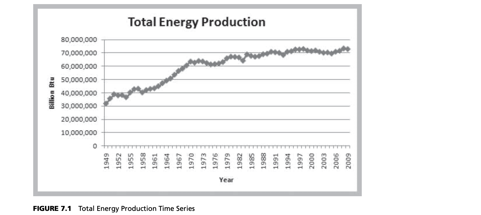
Many forecasts are based on analysis of historical time-series data and are predicated on the assumption that the future is an extrapolation of the past. We will assume that a time series consists of $T$ periods of data, $A_t, t = 1, 2, 3, …, t$. A naive approach is to eyeball a trend—a gradual shift in the value of the time series—by visually examining a plot of the data. For instance, Figure 7.1 shows a chart of total energy production from the data in the Excel file Energy Production & Consumption. We see that energy production was rising quite rapidly during the 1960s; however, the slope appears to have decreased after 1970. It appears that production is increasing by about 500,000 each year and that this can provide a reasonable forecast provided that the trend continues.
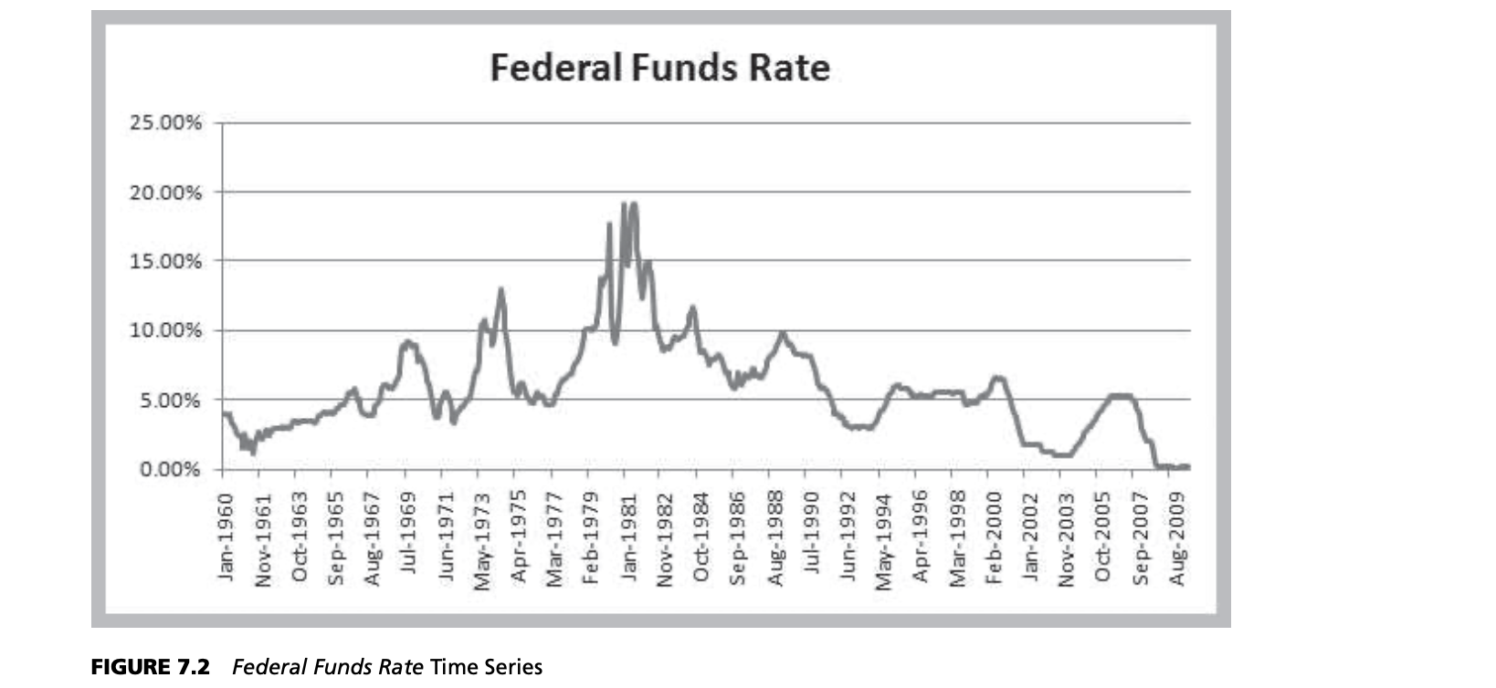
Time series may also exhibit short-term seasonal effects (over a year, month, week, or even a day) as well as longer-term cyclical effects or nonlinear trends. At a neighborhood grocery store, for instance, short-term seasonal patterns may occur over a week, with the heaviest volume of customers on weekends; seasonal patterns may also be evident during the course of a day, with higher volumes in the mornings and late afternoon. Cycles relate to much longer-term behavior, such as periods of inflation and recession or bull and bear stock market behavior. Figure 7.2 shows a chart of the data in the Excel file Federal Funds Rate. We see some evidence of long-term cycles in the time series.
Time Series
- A time series is a stream of historical data
- Components of time series
- Trend
- Short-term seasonal effects
- Longer-term cyclical effects
Excel Support for Forecasting
Among the most popular are moving average methods, exponential smoothing, and regression analysis. These can be implemented very easily on a spreadsheet using basic functions available in Microsoft Excel and its Data Analysis tools;
| Excel Functions | Description |
|---|---|
| TREND (known_y’s, known_x’s, new_x’s, constant) | Returns values along a linear trend line |
| LINEST (known_y’s, known_x’s, new_x’s, constant, stats) | Returns an array that describes a straight line that best fits the data |
| FORECAST (x, known_y’s, known_x’s) | Calculates a future value along a linear trend |
| Analysis Toolpak | Description |
|---|---|
| Moving average | Projects forecast values based on the average value of the variable over a specific number of preceding periods |
| Exponential smoothing | Predicts a value based on the forecast for the prior period, adjusted for the error in that prior forecast |
| Regression | Used to develop a model relating time-series data to a set of variables assumed to influence the data |
FORECASTING MODELS FOR STATIONARY TIME SERIES
Statistical Forecasting Methods
- Moving average
- Exponential smoothing
- Regression analysis
Two simple approaches that are useful over short time periods—when trend, seasonal, or cyclical effects are not significant—are moving average and exponential smoothing models.
Moving Average Models
The simple moving average method is a smoothing method based on the idea of averaging random fluctuations in the time series to identify the underlying direction in which the time series is changing. Because the moving average method assumes that future observations will be similar to the recent past, it is most useful as a short-range forecasting method. Although this method is very simple, it has proven to be quite useful in stable environments, such as inventory management, in which it is necessary to develop forecasts for a large number of items.
Specifically, the simple moving average forecast for the next period is computed as the average of the most recent $k$ observations. The value of $k$ is somewhat arbitrary, although its choice affects the accuracy of the forecast. The larger the value of $k$, the more the current forecast is dependent on older data and the forecast will not react as quickly to fluctuations in the time series. The smaller the value of $k$, the quicker the forecast responds to changes in the time series. Also, when $k$ is larger, extreme values have less effect on the forecasts. (In the next section, we discuss how to select $k$ by examining errors associated with different values.)
- Average random fluctuations in a time series to infer short-term changes in direction
- Assumption: future observations will be similar to recent past
- Moving average for next period = average of most recent $k$ observations
Example
For instance, suppose that we want to forecast monthly burglaries from the Excel file Burglaries since the citizen-police program began. Figure 7.3 shows a chart of these data. The time series appears to be relatively stable, without trend, seasonal, or cyclical effects; thus, a moving average model would be appropriate. Setting $k = 3$, the three-period moving average forecast for month 59 is:
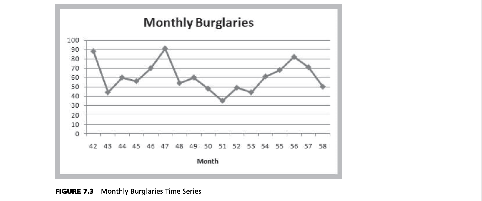
$$Month \space 59 \space forecast = \frac{82+71+50}{3} = 67.67$$
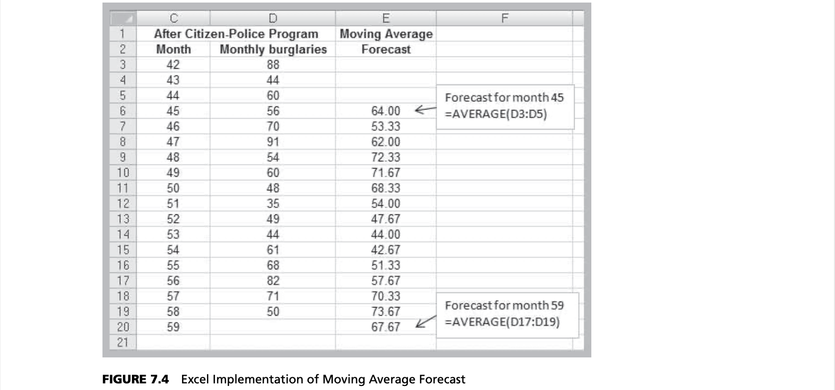
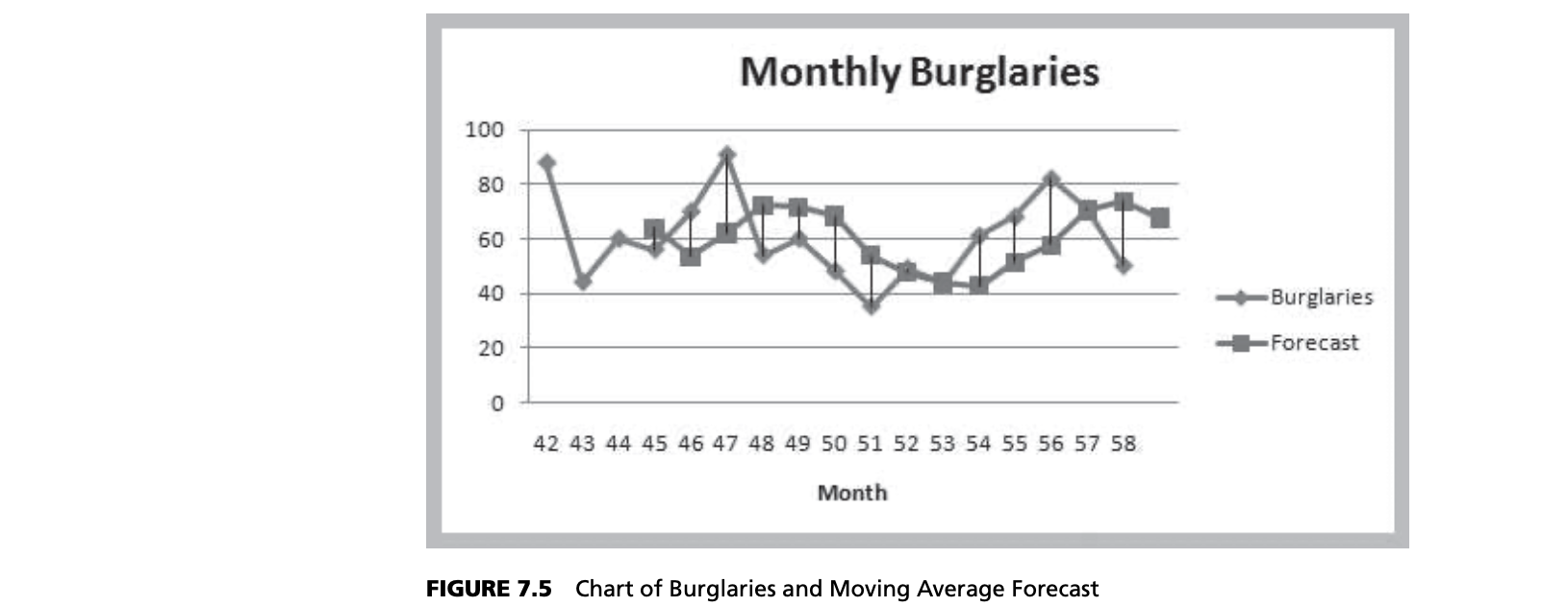
Moving average forecasts can be generated easily on a spreadsheet. Figure 7.4 shows the computations for a three-period moving average forecast of burglaries. Figure 7.5 shows a chart that contrasts the data with the forecasted values. Moving average forecasts can also be obtained from Excel’s Data Analysis options (see Appendix 7.2A, Forecasting with Moving Averages).
Time Series Data and Moving Averages
In the simple moving average approach, the data are weighted equally. This may not be desirable because we might wish to put more weight on recent observations than on older observations, particularly if the time series is changing rapidly. Such models are called weighted moving averages. For example, you might assign a 60% weight to the most recent observation, 30% to the second most recent observation, and the remain- ing 10% of the weight to the third most recent observation. In this case, the three-period weighted moving average forecast for month 59 would be:
$$Month \space 59 \space forecast = \frac{0.1 \times 82+0.3 \times 71+0.6 \times 50}{0.1+0.3+0.6} = \frac{59.5}{1} = 59.5$$
Error Metrics and Forecast Accuracy
The quality of a forecast depends on how accurate it is in predicting future values of a time series. The error in a forecast is the difference between the forecast and the actual value of the time series (once it is known!). In Figure 7.5, the forecast error is simply the vertical distance between the forecast and the data for the same time period. In the simple moving average model, different values for $k$ will produce different forecasts.
How do we know, for example, if a two- or three-period moving average forecast or a three-period weighted moving average model (or others) would be the best predictor for burglaries? We might first generate different forecasts using each of these models, as shown in Figure 7.6, and compute the errors associated with each model.
To analyze the accuracy of these models, we can define error metrics, which compare quantitatively the forecast with the actual observations. Three metrics that are commonly used are the mean absolute deviation, mean square error, and mean absolute percentage error. The mean absolute deviation (MAD) is the absolute difference between the actual value and the forecast, averaged over a range of forecasted values:
$$\displaystyle MAD = \frac{\sum^{n}_{t=1}|A_t - F_t|}{n}$$
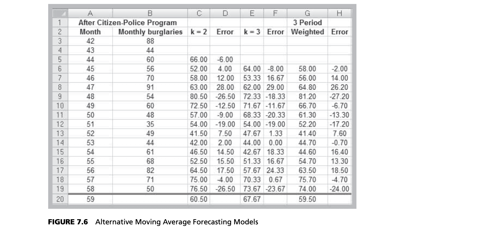
where $A_t$ is the actual value of the time series at time $t$, $F_t$ is the forecast value for time $t$, and $n$ is the number of forecast values (not the number of data points since we do not have a forecast value associated with the first $k$ data points). MAD provides a robust measure of error and is less affected by extreme observations.
Mean square error (MSE) is probably the most commonly used error metric. It penalizes larger errors because squaring larger numbers has a greater impact than squaring smaller numbers. The formula for MSE is:
$$\displaystyle MSE = \frac{\sum^{n}_{t=1}(A_t - F_t)^2}{n}$$
Again, $n$ represents the number of forecast values used in computing the average. Sometimes the square root of MSE, calle the root mean square error (RMSE), is used:
$$\displaystyle RMSE = \sqrt{\frac{\sum^{n}_{t=1}(A_t - F_t)^2}{n}}$$
Note that unlike MSE, RMSE is expressed in the same units as the data (similar to the difference between a standard deviation and a variance), allowing for more practical comparisons.
A fourth commonly used metric is mean absolute percentage error (MAPE). MAPE is the average of absolute errors divided by actual observation values.
$$\displaystyle MAPE = \frac{\sum^{n}_{t=1}|\frac{A_t - F_t}{A_t}|}{n} \times 100%$$
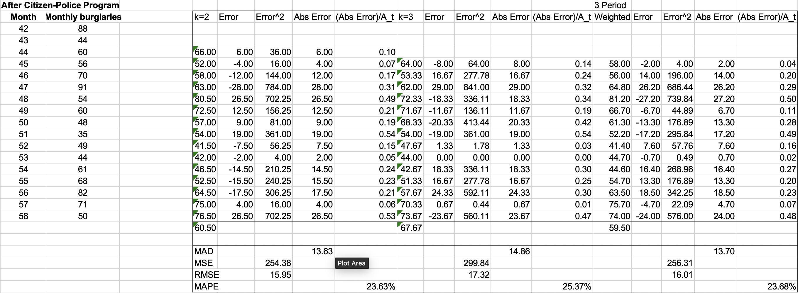
The values of MAD and MSE depend on the measurement scale of the time-series data. For example, forecasting profit in the range of millions of dollars would result in very large MAD and MSE values, even for very accurate forecasting models. On the other hand, market share is measured in proportions; therefore, even bad forecasting models will have small values of MAD and MSE. Thus, these measures have no meaning except in comparison with other models used to forecast the same data. Generally, MAD is less affected by extreme observations and is preferable to MSE if such extreme observations are considered rare events with no special meaning. MAPE is different in that the measurement scale is eliminated by dividing the absolute error by the time-series data value. This allows a better relative comparison. Although these comments provide some guidelines, there is no universal agreement on which measure is best.
Exponential Smoothing Models
A versatile, yet highly effective approach for short-range forecasting is simple exponential smoothing. The basic simple exponential smoothing model is:
$$F_{t+1} = (1-a)F_t + aA_t = F_t + a(A_t - F_t)$$
- $F_{t+1}$ is the forecast for time period $t+1$,
- $F_t$ is the forecast for period $t$,
- $A_t$ is the observed value in period $t$, and
- $a$ is a constant between 0 and 1, called the smoothing constant.
For the burglary data, the forecast for month 43 is 88, which is the actual observation for month 42. Suppose we choose $a = 0 .7$; then the forecast for month 44 would be:
$$Month \space 44 \space Forecast = (1 - 0.7)(88) + (0.7)(44) = 57.2$$
Since the simple exponential smoothing model requires only the previous forecast and the current time-series value, it is very easy to calculate; thus, it is highly suitable for environments such as inventory systems where many forecasts must be made. The smoothing constant $a$ is usually chosen by experimentation in the same manner as choosing the number of periods to use in the moving average model. Different values of a affect how quickly the model responds to changes in the time series. For instance, a value of $a = 0$ would simply repeat last period’s forecast, while $a = 1$ would forecast last period’s actual demand. The closer $a$ is to 1, the quicker the model responds to changes in the time series because it puts more weight on the actual current observation than on the forecast. Likewise, the closer a is to 0, the more weight is put on the prior forecast, so the model would respond to changes more slowly.
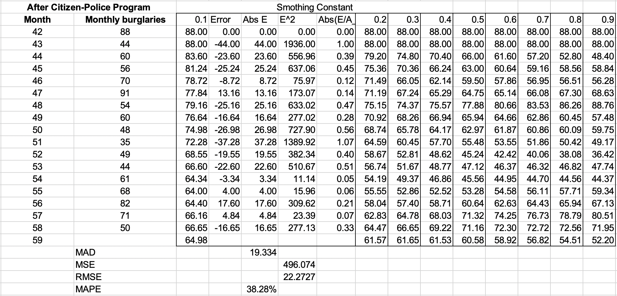
Adjusted Exponential Smoothing
Trend for the previous Exponential Smoothing.
$$AF_{t} = F_{t}+T_{t}$$
$$T_{t} = \beta(F_{t} - F_{t-1})+(1 - \beta)T_{t-1}$$
- $T$: the trend between zero to one exclusive.
- $AF_t$: the adjusted exponential smoothing
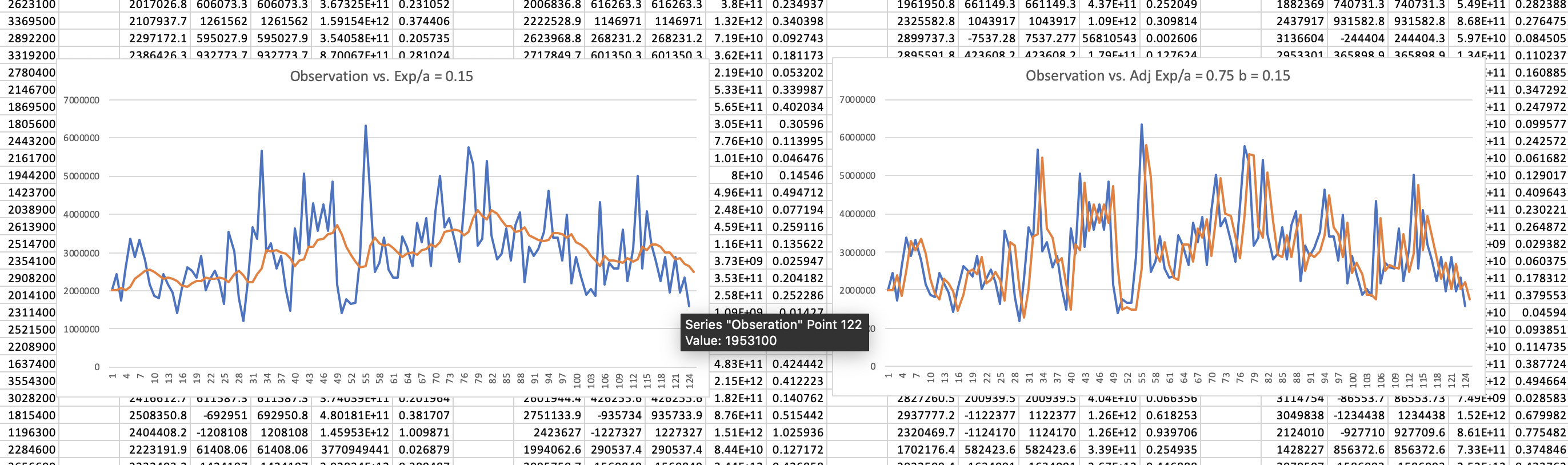
FORECASTING MODELS FOR TIME SERIES WITH A LINEAR TREND
For time series with a linear trend but no significant seasonal components, double moving average and double exponential smoothing models are more appropriate than using simple moving average or exponential smoothing models. Both methods are based on the linear trend equation:
- Double Moving Average
- Double Exponential Smoothing
- Based on the linear trend equation
$$F_{t+k} = a_t + b_t k$$
That is, the forecast for $k$ periods into the future from period $t$ is a function of a base value $a_t$, also known as the level, and a trend, or slope, $b_t$ . Double moving average and double exponential smoothing differ in how the data are used to arrive at appropriate values for $a_t$ and $b_t$.
Regression-Based Forecasting
$F_{t+k} = a_t + b_t k$ may look familiar from simple linear regression that is a means of developing relationships between dependent and independent variables. Simple linear regression can be applied to forecasting using time as the independent variable.
For example, Figure 7.8 shows a portion of the Excel file Coal Production, which provides data on total tons produced from 1960 through 2007. A linear trendline shows an $R^2$ value of 0.969 (the fitted model assumes that the years are numbered 1 through 48, not as actual dates). The actual values of the coefficients in
the model are shown below:
$$Tons = 416,896,322.7 + 16,685,398.57 \times Year$$
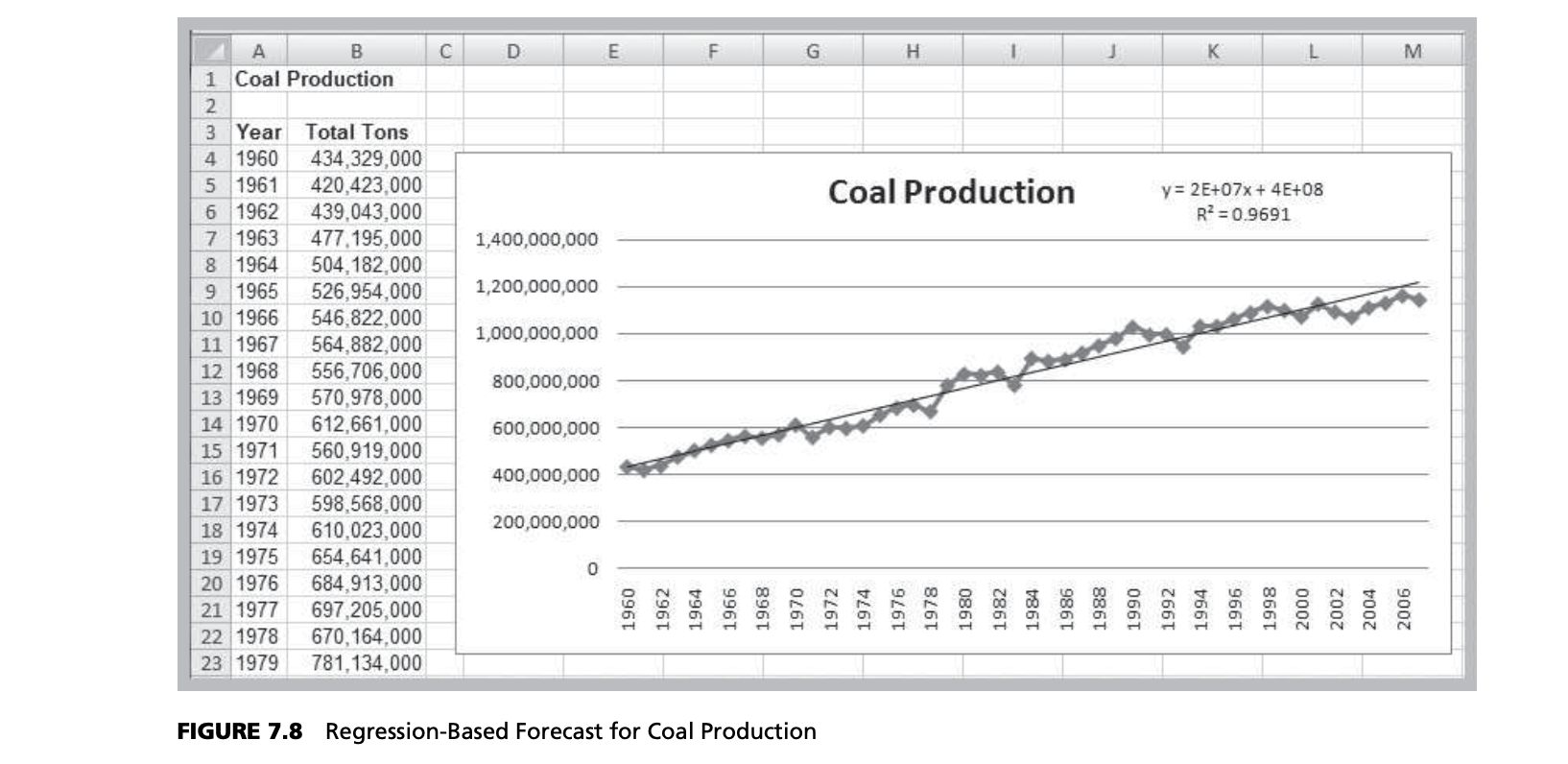
Thus, a forecast for 2008 would be:
$$Tons = 416,896,322.7 + 16,685,398.57 \times (49) = 1,234,480,853$$
ADVANCED FORECASTING MODELS
In Chapter 6, we noted that an important assumption for using regression analysis is the lack of autocorrelation among the data. When autocorrelation is present, successive observations are correlated with one another; for example, large observations tend to follow other large observations, and small observations also tend to follow one another. This can often be seen by examining the residual plot when the data are ordered by time. Figure 7.9 shows the time-ordered residual plot from PHStat for the coal production regression. The residuals do not appear to be random; rather, successive observations seem to be related to one another. We introduced the Durbin–Watson statistic in Chapter 6 as a means of evaluating autocorrelation. From the PHStat regression tool, the Durbin–Watson statistic was computed to be 0.768, which suggests autocorrelation, indicating that other approaches, called autoregressive models, are more appropriate.
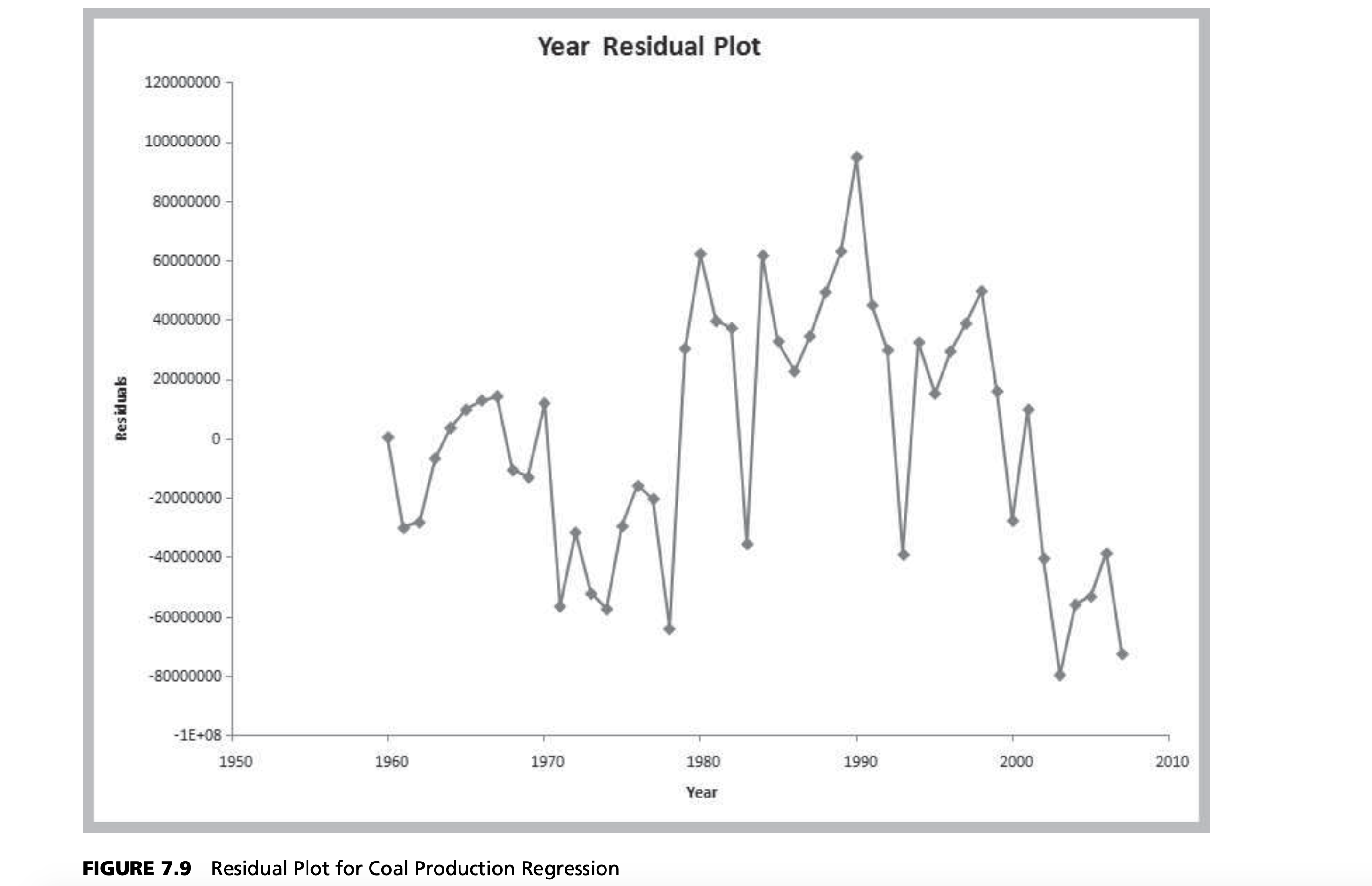
Autoregressive Forecasting Models
An autoregressive forecasting model incorporates correlations between consecutive values in a time series by using explanatory variables that are lagged values of the dependent variable. A first-order autocorrelation refers to the correlation among data values one period apart, a second-order autocorrelation refers to the correlation among data values two periods apart, and so on. Autoregressive models improve forecasting when autocorrelation is present in data. A first-order autoregressive model is:
$$Y_i = a_0 + a_1Y_{i-1} + \delta_i$$
where $Y_i$ is the value of the time series in period $i$ and $\delta_i$ is a nonautocorrelated random error term having 0 mean and constant variance. A second-order autoregressive model is:
$$Y_i = a_0 + a_1Y_{i-1} + a_2Y_{i-2} + \delta_i$$
Additional terms may be added for higher-order models.
To build an autoregressive model using multiple linear regression, we simply add
additional columns to the data matrix for the dependent variable that lag the original data by some number of periods. Thus, for a third-order autoregressive model, we add columns that lag the dependent variable by one, two, and three periods. For the coal production data, a portion of this data matrix is shown in Figure 7.10. However, we must be careful to use the appropriate data when running the regression models. For example, to run a third-order model, we must not include the first three rows of the matrix, since there are no Lag 3 values for those years. Similarly, for a second-order model, do not include the data for the first two rows.
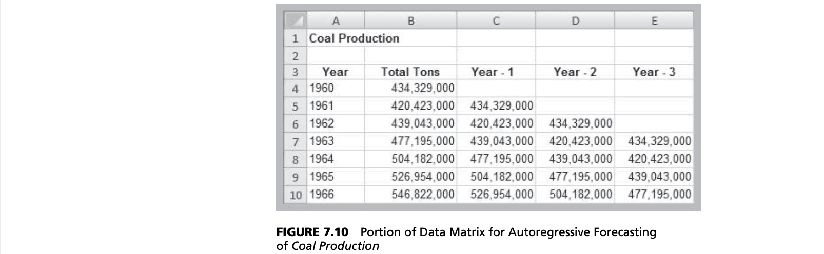
Example
Suppose that we try a third-order model first. Using the multiple regression tool, we obtain the results shown in Figure 7.11. Note that the largest p-value (for the third-order term) exceeds $a = 0.05$, indicating that this variable is not significant. Dropping it and re-running a second-order model yields the results shown in Figure 7.12. Thus, we can use the second-order model to forecast the coal production:
$$Tons = 43,087,157 + 0.632 \times Tons_{Year-1} + 0.341 \times Tons_{Year-2}$$
A forecast for the year 2008 would be:
$$Tons = 43,087,157 + 0.632 \times Tons_{2007} + 0.341 \times Tons_{2006}$$
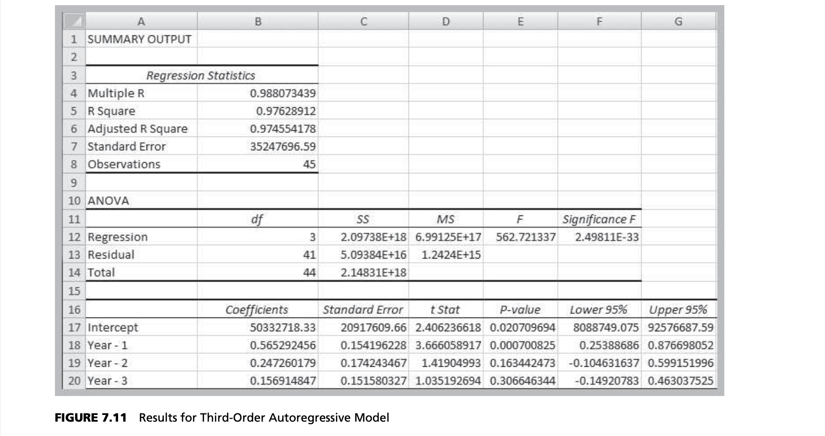
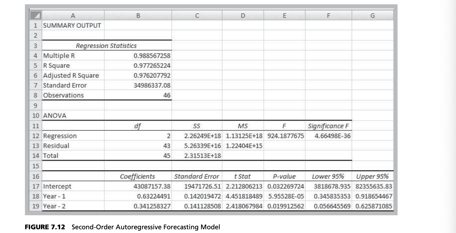
Forecasting Models with Seasonality 252
Incorporating Seasonality in Regression Models 253
Forecasting Models with Trend and Seasonality
Regression Forecasting with Causal Variables 255
CHOOSING AND OPTIMIZING FORECASTING MODELS USING CB PREDICTOR 257
THE PRACTICE OF FORECASTING 262
BASIC CONCEPTS REVIEW QUESTIONS 263
PROBLEMS AND APPLICATIONS 264
CASE: ENERGY FORECASTING 265
APPENDIX 7.1: ADVANCED FORECASTING MODELS—THEORY AND COMPUTATION 265
Double Moving Average 265
Double Exponential Smoothing 265
Additive Seasonality 266
Multiplicative Seasonality 266
Holt–Winters Additive Model 266
Holt–Winters Multiplicative Model 267
APPENDIX 7.2: EXCEL AND CB PREDICTOR NOTES 267
A. Forecasting with Moving Averages 267
B. Forecasting with Exponential Smoothing 267
C. Using CB Predictor 268
CHAPTER 9: BUILDING AND USING DECISION MODELS
SUMMARY
建模是一种通过变量进行决策的技术, 复数或相互依赖的变量会提高模型的复杂度.
INTRODUCTION
Everyone makes decisions. Individuals face personal decisions such as choosing a college or graduate program, making product purchases, selecting a mortgage instrument, and investing for retirement. Managers in business organizations must determine what products to make and how to price them, where to locate facilities, how many people to hire, where to allocate advertising budgets, whether or not to outsource a business function, and how to schedule production. Developing effective strategies to deal with these types of problems can be a difficult task. Quantitative decision models can greatly assist in these types of decisions. Part II of this book is devoted to the development and application of decision models.
Spreadsheets, in particular, provide a convenient means to manage data, construct models, and analyze them for gaining insight and supporting decisions. Although the early applications of spreadsheets were primarily in accounting and finance, spreadsheets have developed into powerful general-purpose managerial tools for decision modeling and analysis.
DECISION MODELS
- A model is an abstraction or representation of a real system, idea, or object.
- Data, which are assumed to be constant for purposes of the model. Some examples would be costs, machine capacities, and intercity distances.
- Uncontrollable variables, which are quantities that can change but cannot be directly controlled by the decision maker. Some examples would be customer demand, inflation rates, and investment returns.
- Decision variables, which are controllable and can be selected at the discretion of the decision maker. Some examples would be production quantities, staffing levels, and investment allocations.
- Models could be pictures, spreadsheets, or mathematical relationships
- Models contain data, uncontrollable variables, and decision variables

Example
Suppose that a manufacturer can produce a part for $125/unit with a fixed cost of $50,000. The alternative is to outsource production to a supplier at a unit cost of $175. The decision depends on the anticipated volume of demand; for high volumes, the cost to manufacture in-house will be lower than outsourcing, because the fixed costs can be spread over a large number of units. For small volumes, it would be more economical to outsource. Knowing the cost of both alternatives and the breakeven point would facilitate the decision. The data consist of the costs associated with manufacturing the product in-house or purchasing it from an outside supplier. The key model input is the demand volume and the outputs are the total manufacturing and purchase cost. Calculating the outputs basically consists of “stepping through” the formulas.
This model can also be expressed mathematically by defining symbols for each component of the model:
- F = fixed cost of in-house manufacturing
- V = unit variable cost of in-house manufacturing
- C = unit cost of outsourcing
- D = demand volume
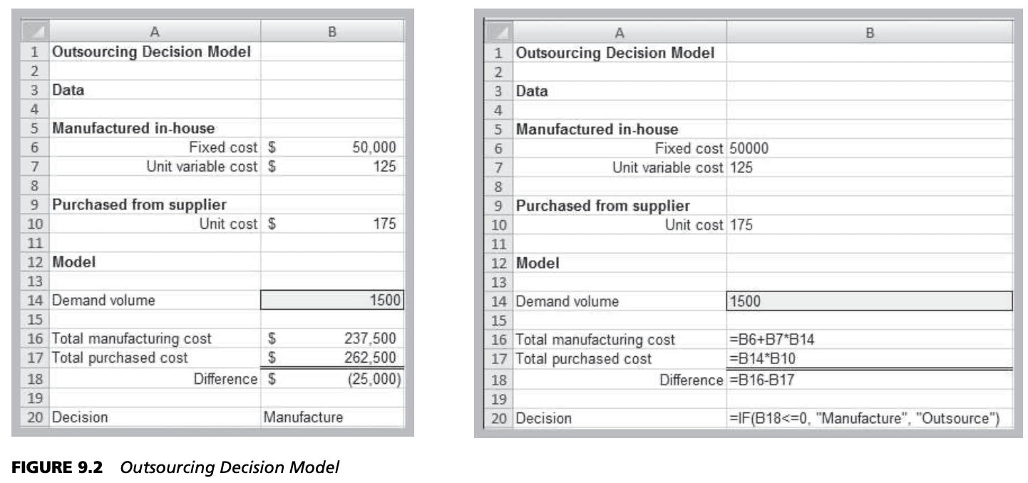
Then the total manufacturing cost can be written as $TMC = F + V \times D$, and the total outsourcing cost as $TOC = C \times D$.Note the correspondence between the spreadsheet formulas and the mathematical model:
$$TMC = B6 + B7*B14$$
$$TOC = B14 * B10$$
Thus, if you can write a spreadsheet formula, you can develop a mathematical model! Mathematical models are easy to manipulate; for example, it is easy to find the
breakeven volume by setting TMC = TOC and solving for D:
$$F+VD=CD$$
$$D = F>(C - V)$$
In contrast, it is more difficult to find the breakeven volume using trial-and-error on the spreadsheet without knowing some advanced tools and approaches. However, spread-sheets have the advantage of allowing you to easily modify the model inputs and calculate the numerical results. We will use both spreadsheets and analytical modeling approaches in our model-building applications, and it is important to be able to “speak both languages.”
Outsourcing Model
- Model components
- F = fixed cost of in-house manufacturing
- V = unit variable cost of in-house manufacturing
- C = unit cost of outsourcing
- D = demand volume
- Total Manufacturing Cost = $TMC = F + V * D$
- Total outsourcing cost = $TOC = C * D$.
MODEL ANALYSIS 299
What-If Analysis 299
One-way data table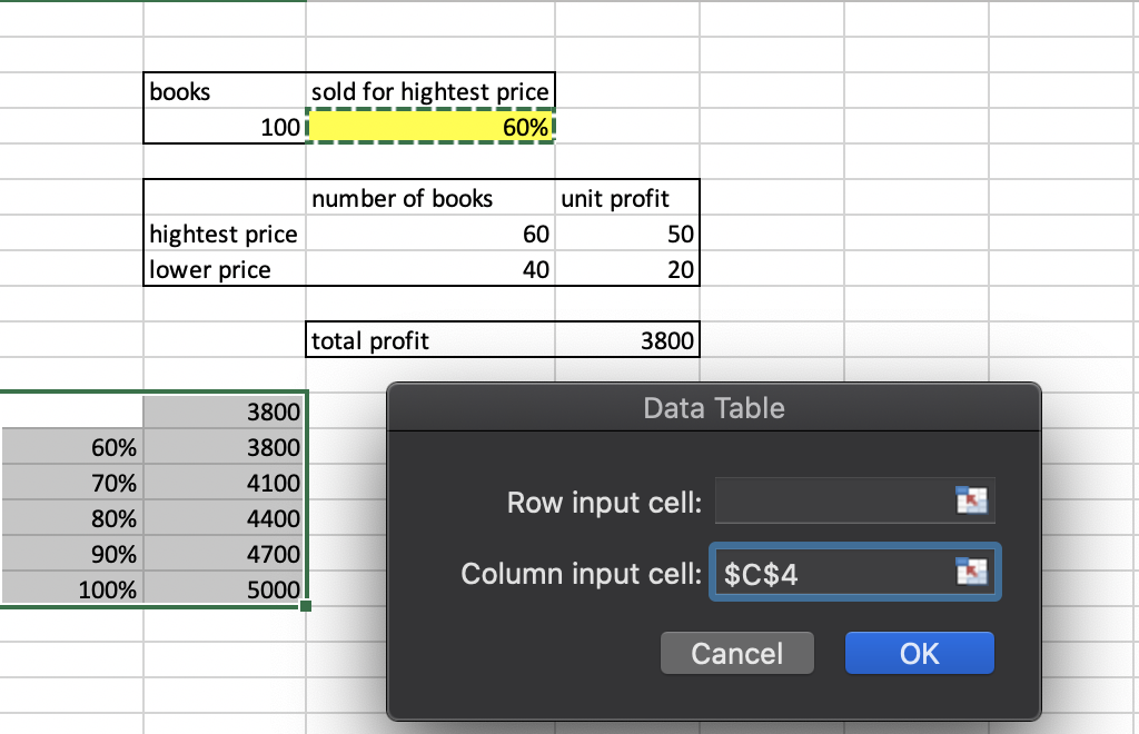
- 下面的数据需要引用上面的数据, 不能直接输入, 比如 number of books
- 百分比不能用前一个数据相加, 必须手动输入(尚不清楚原因, 否则会计算出错误结果)
https://www.excel-easy.com/examples/data-tables.html
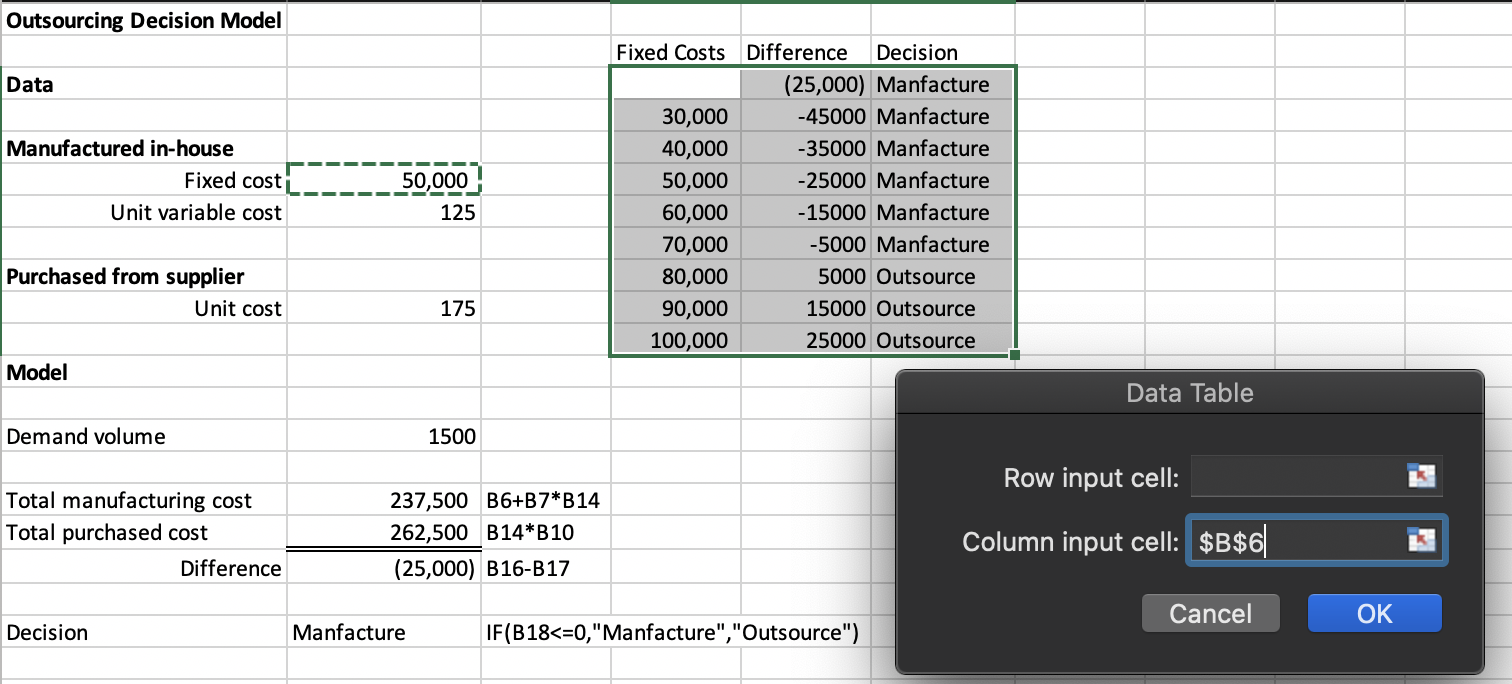
Two-way data table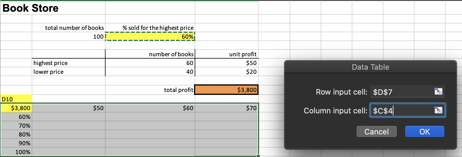
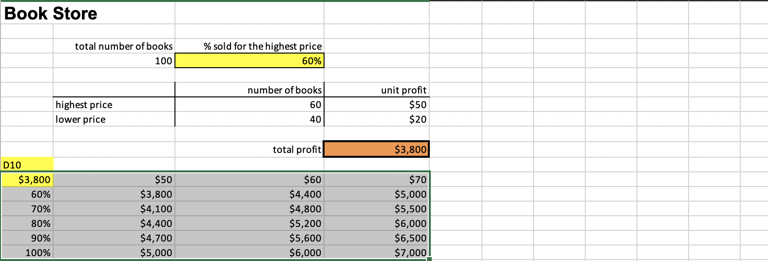
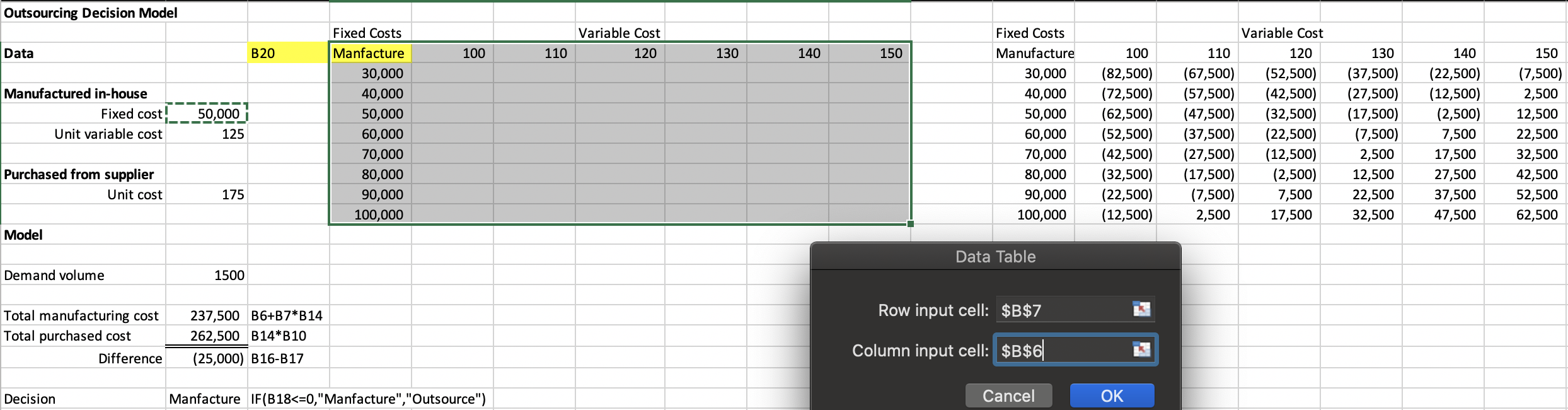
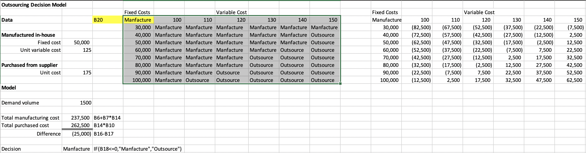
Model Optimization 302
TOOLS FOR MODEL BUILDING 304
Logic and Business Principles 304
Common Mathematical Functions 305 n Data Fitting 306
Spreadsheet Engineering 308
SPREADSHEET MODELING EXAMPLES 309 n New Product Development 309
Single Period Purchase Decisions 311
Overbooking Decisions 312
Project Management 313
MODEL ASSUMPTIONS, COMPLEXITY, AND REALISM 315
BASIC CONCEPTS REVIEW QUESTIONS 317
PROBLEMS AND APPLICATIONS 318
CASE: AN INVENTORY MANAGEMENT DECISION MODEL 321
APPENDIX 9.1: EXCEL NOTES 322
A. Creating Data Tables 322
B. Using the Scenario Manager 322
C. Using Goal Seek 323
D. Net Present Value and the NPV Function 323
- 42.Technically speaking, computers cannot generate truly random numbers since they must use a predictable algorithm. ↩
- 372.For continuous random variables, it does not make mathematical sense to attempt to define a probability for a specific value of x because there are an infinite number of values; thus, $P(X = x) = 0$. For continuous random variables, probabilities are only defined over intervals, such as $P(a ≤ X ≤ b), P(X < c), or \space P(X > d)$. ↩
- 377.The triangular distribution is often used as a rough approximation of other distributions, such as the normal, or when no data are available and a distribution must be assumed judgmentally. Because it depends on three simple parameters and can assume a variety of shapes—for instance, it can be skewed in either direction by changing the value of c—it is very flexible in modeling a wide variety of assumptions. One drawback, however, is that it is bounded, thereby eliminating the possibility of extreme values that might possibly occur. Excel does not have a function to compute triangular probabilities. ↩
- 431.For example, consider a normal population with mean $\mu$ and variance $\sigma ^{2}$. Assume we repeatedly take samples of a given size from this population and calculate the arithmetic mean ${\bar x}$ for each sample – this statistic is called the sample mean. The distribution of these means, or averages, is called the "sampling distribution of the sample mean" ↩
- 3762.If cumulative is set to FALSE, the function simply calculates the value of the density function $f(x)$, which has little practical application. ↩
- 3771.Outcomes near the most likely value have a higher chance of occurring than those at the extremes. ↩
- 4131.For example, to sample 250 names from a list of 400,000, the first name could be selected at random from the first 1,600, and then every 1,600th name could be selected. This approach can be used for telephone sampling when supported by an automatic dialer that is programmed to dial numbers in a systematic manner. However, systematic sampling is not the same as simple ran- dom sampling because for any sample, every possible sample of a given size in the population does not have an equal chance of being selected. In some situations, this approach can induce significant bias if the population has some underlying pattern. For instance, sampling orders received every seven days may not yield a representative sample if customers tend to send orders on certain days every week. ↩
- 4132.For example, a large city may be divided into political districts called wards. Each ward has a different number of citizens. A stratified sample would choose a sample of individuals in each ward proportionate to its size. This approach ensures that each stratum is weighted by its size relative to the population and can provide better results than simple random sampling if the items in each stratum are not homogeneous. However, issues of cost or significance of certain strata might make a disproportionate sample more useful. For example, the ethnic or racial mix of each ward might be significantly different, making it difficult for a stratified sample to obtain the desired information. ↩
- 4133.For instance, a company might segment its customers into small geographical regions. A cluster sample would consist of a random sample of the geographical regions, and all customers within these regions would be surveyed (which might be easier because regional lists might be easier to produce and mail). ↩
- 4134.First, select a time at random; then select the next n items produced after that time. Second, select n times at random; then select the next item produced after these times. The first approach generally ensures that the observations will come from a homogeneous population; however, the second approach might include items from different populations if the characteristics of the process should change over time, so caution should be used. ↩