R Tutorial
Introduction
read.table {utils}
Description
Reads a file in table format and creates a data frame from it, with cases corresponding to lines and variables to fields in the file.
Usage
1 | read.table(file, header = FALSE, sep = "", quote = "\"'", |
Arguments
1 | file |
Example
aggregate {stats}
Description
Splits the data into subsets, computes summary statistics for each, and returns the result in a convenient form.
将数据拆分为子集, 计算每个子集的摘要统计信息, 并以方便的形式返回结果.
Usage
1 | aggregate(x, ...) |
Example
1 | > d <- read.csv("Global Superstore Orders 2016(1).csv") |
Plot {graphics}
Description
1 | Generic function for plotting of R objects. For more details about the graphical parameter arguments, see par. |
Usage
1 | plot(x, y, ...) |
Arguments
1 | x |
Example
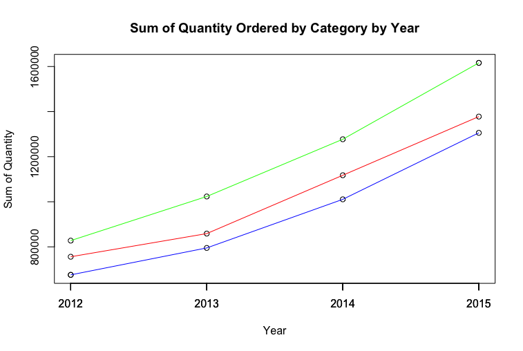
1 | # aggregate() 将 d$Sales 以 d$Category, d$Order.Year 分组, 并将各组数据求和. 得到了原来没有的新数据组合. |
1 | # axis() 修改坐标轴, 1 的意思是修改下面(x axis). at 以哪个点修改. |
1 | # points() 在坐标轴上加点, 左边是 x 值, 右边是 y 值. |
1 | # lines() 在坐标轴上画线, 并区分颜色. |