R Shiny
Reference
The basic parts of a Shiny app
24 beautifully-designed web dashboards that data geeks will love
Introduction
Let’s walk through the steps of building a simple Shiny application. A Shiny application is simply a directory containing an R script called app.R which is made up of a user interface object and a server function. This folder can also contain any any additional data, scripts, or other resources required to support the application.
ui
fluidPage: If you are creating a shiny application, the best way to ensure that the application interface runs smoothly on different devices with different screen resolutions is to create it using fluid page. This ensures that the page is laid out dynamically based on the resolution of each device.

The user interface can be broadly divided into three categories:
- Title Panel: The content in the title panel is displayed as metadata, as in top left corner of above image which generally provides name of the application and some other relevant information.
- Sidebar Layout: Sidebar layout takes input from the user in various forms like text input, checkbox input, radio button input, drop down input, etc. It is represented in dark background in left section of the above image.
- Main Panel: It is part of screen where the output(s) generated as a result of performing a set of operations on input(s) at the server.R is / are displayed.
1 | #UI.R |
server
This acts as the brain of web application. The server.R is written in the form of a function which maps input(s) to the output(s) by some set of logical operations. The inputs taken in ui.R file are accessed using $ operator (input$InputName). The outputs are also referred using the $ operator (output$OutputName). We will be discussing a few examples of server.R in the coming sections of the article for better understanding.
1 | #SERVER.R |
Advantages and Disadvantages of Shiny
There are plenty of other data visualization tools out there. So, to help you compare what differentiates Shiny and what you can and cannot do with Shiny, let’s look at the advantages and disadvantages of using shiny.
Advantages :
- Efficient Response Time: The response time of shiny app is very small, making it possible to deliver real time output(s) for the given input.
- Complete Automation of the app: A shiny app can be automated to perform a set of operations to produce the desire output based on input.
- Knowledge of HTML, CSS or JavaScript not required: It requires absolutely no prior knowledge of HTML, CSS or JavaScript to create a fully functional shiny app.
- Advance Analytics: Shiny app is very powerful and can be used to visualize even the most complex of data like 3D plots, maps, etc.
- Cost effective: The paid versions of shinyapps.io and shiny servers provide a cost effective scalable solution for deployment of shiny apps online.
- Open Source: Building and getting a shiny app online is free of cost, if you wish to deploy your app on the free version of shinyapps.io
Disadvantages :
- Requires timely updates: As the functions used in the app gets outdated sometimes with newer package versions, it becomes necessary to update your shiny app time to time.
- No selective access and permissions: There’s no provision for blocking someone’s access to your app or proving selective access. Once the app is live on the web, it is freely accessible by everyone
- Restriction on traffic in free version: In free version of shinyapps.io, you only get 25 active hours of your app per month per account.
Basic ui & server
1 | # Basic UI |
1 | # Basic Server |
1 | # Shiny App |
UI & Server
To get started building the application, create a new empty directory wherever you’d like, then create an empty app.R file within it. For purposes of illustration we’ll assume you’ve chosen to create the application at ~/shinyapp:
1 | ~/shinyapp |
Now we’ll add the minimal code required in the source file called app.R.
First, we load the shiny package:
1 | library(shiny) |
ui
Then, we define the user interface by calling the function pageWithSidebar:
1 | # Define UI for miles per gallon app ---- |
The three functions headerPanel, sidebarPanel, and mainPanel define the various regions of the user-interface. The application will be called “Miles Per Gallon” so we specify that as the title when we create the header panel. The other panels are empty for now.
Now let’s define a skeletal server implementation. To do this we call shinyServer and pass it a function that accepts two parameters, input and output:
server
1 | # Define server logic to plot various variables against mpg ---- |
Our server function is empty for now but later we’ll use it to define the relationship between our inputs and outputs.
app.R
Finally, we need the shinyApp function that uses the ui object and the server function we defined to build a Shiny app object.
Putting it altogether, our app.R script looks like this:
1 | library(shiny) |
We’ve now created the most minimal possible Shiny application. You can run the application by calling the runApp function as follows
1 | > library(shiny) |
Alternatively, if you are working on you can click the Run App button on your RStudio Editor.
If everything is working correctly you’ll see the application appear in your browser looking something like this:
![]()
We now have a running Shiny application however it doesn’t do much yet. In the next section we’ll complete the application by specifying the user interface object and implementing the server function
Inputs & Outputs
Adding Inputs to the Sidebar
The application we’ll be building uses the mtcars data from the R datasets package, and allows users to see a box-plot that explores the relationship between miles-per-gallon (MPG) and three other variables (Cylinders, Transmission, and Gears).
We want to provide a way to select which variable to plot MPG against as well as provide an option to include or exclude outliers from the plot. To do this we’ll add two elements to the sidebar, a selectInput to specify the variable and a checkboxInput to control display of outliers. Our user-interface definition looks like this after adding these elements:
ui
1 | # Define UI for miles per gallon app ---- |
If you run the application again after making these changes you’ll see the two user-inputs we defined displayed within the sidebar:

Creating the server function
Next we need to define the server-side of the application which will accept inputs and compute outputs. Our server function is shown below, and illustrates some important concepts:
- Accessing input using slots on the
inputobject and generating output by assigning to slots on theoutputobject. - Initializing data at startup that can be accessed throughout the lifetime of the application.
- Using a reactive expression to compute a value shared by more than one output.
The basic task of a Shiny server function is to define the relationship between inputs and outputs. Our function does this by accessing inputs to perform computations and by assigning reactive expressions to output slots.
Here is the source code for the full server function (the inline comments explain the implementation techniques in more detail):
server
1 | # Data pre-processing ---- |
The use of renderText and renderPlot to generate output (rather than just assigning values directly) is what makes the application reactive. These reactive wrappers return special expressions that are only re-executed when their dependencies change. This behavior is what enables Shiny to automatically update output whenever input changes.
Displaying Outputs
The server function assigned two output values: output$caption and output$mpgPlot. To update our user interface to display the output we need to add some elements to the main UI panel.
In the updated user-interface definition below you can see that we’ve added the caption as an h3 element and filled in its value using the textOutput function, and also rendered the plot by calling the plotOutput function:
ui
1 | # Define UI for miles per gallon app ---- |
Running the application now shows it in its final form including inputs and dynamically updating outputs:

Details
The shinyApp() function returns an object of class shiny.appobj. When this is returned to the console, it is printed using the print.shiny.appobj() function, which launches a Shiny app from that object.
You can also use a similar technique to create and run files that aren’t named app.R and don’t reside in their own directory. If, for example, you create a file called test.R and have it call shinyApp() at the end, you could then run it from the console with:
1 | print(source("test.R")) |
When the file is sourced, it returns a shiny.appobj — but by default, the return value from source() isn’t printed. Wrapping it in print() causes Shiny to launch it.
This method is handy for quick experiments, but it lacks some advantages that you get from having an app.R in its own directory. When you do runApp("newdir"), Shiny will monitor the file for changes and reload the app if you reload your browser, which is useful for development. This doesn’t happen when you simply source the file. Also, Shiny Server and shinyapps.io expect an app to be in its own directory. So if you want to deploy your app, it should go in its own directory.
Now that we’ve got a simple application running we’ll probably want to make some changes. The next article covers the basic cycle of editing, running, and debugging Shiny applications.
app.R
1 | # Define UI for miles per gallon app ---- |
Example
The basic parts of a Shiny app
The Shiny package comes with eleven built-in examples that demonstrate how Shiny works. This article reviews the first three examples, which demonstrate the basic structure of a Shiny app.
Example 1: Hello Shiny

The Hello Shiny example is a simple application that plots R’s built-in faithful dataset with a configurable number of bins. To run the example, type:
1 | library(shiny) |
Shiny applications have ==two components==, a user interface object and a server function, that are passed as arguments to the shinyApp function that creates a Shiny app object from this UI/server pair. The source code for both of these components is listed below.
In subsequent sections of the article we’ll break down Shiny code in detail and explain the use of “reactive” expressions for generating output. For now, though, just try playing with the sample application and reviewing the source code to get an initial feel for things. Be sure to read the comments carefully.
The user interface is defined as follows:
1 | # Define UI for app that draws a histogram ---- |
The server-side of the application is shown below. At one level, it’s very simple – a random distribution is plotted as a histogram with the requested number of bins. However, you’ll also notice that the code that generates the plot is wrapped in a call to renderPlot. The comment above the function explains a bit about this, but if you find it confusing, don’t worry, we’ll cover this concept in much more detail soon.
1 | # Define server logic required to draw a histogram ---- |
Finally, we use the shinyApp function to create a Shiny app object from the UI/server pair that we defined above.
1 | # Create Shiny app ---- |
We save all of this code, the ui object, the server function, and the call to the shinyApp function, in an R script called app.R. This is the same basic structure for all Shiny applications.
The next example will show the use of more input controls, as well as the use of reactive functions to generate textual output.
Example 2: Shiny Text

The Shiny Text application demonstrates printing R objects directly, as well as displaying data frames using HTML tables. To run the example, type:
1 | library(shiny) |
The first example had a single numeric input specified using a slider and a single plot output. This example has a bit more going on: two inputs and two types of textual output.
If you try changing the number of observations to another value, you’ll see a demonstration of one of the most important attributes of Shiny applications: inputs and outputs are connected together “live” and changes are propagated immediately (like a spreadsheet). In this case, rather than the entire page being reloaded, just the table view is updated when the number of observations change.
Here is the user interface object for the application. Notice in particular that the sidebarPanel and mainPanel functions are now called with two arguments (corresponding to the two inputs and two outputs displayed):
1 | # Define UI for dataset viewer app ---- |
The server side of the application has also gotten a bit more complicated. Now we create:
- A reactive expression to return the dataset corresponding to the user choice
- Two other rendering expressions (
renderPrintandrenderTable) that return theoutput$summaryandoutput$viewvalues
These expressions work similarly to the renderPlot expression used in the first example: by declaring a rendering expression you tell Shiny that it should only be executed when its dependencies change. In this case that’s either one of the user input values (input$dataset or input$obs).
1 | # Define server logic to summarize and view selected dataset ---- |
Example 3: Reactivity

The Reactivity application is very similar to Hello Text, but goes into much more detail about reactive programming concepts. To run the example, type:
1 | library(shiny) |
The previous examples have given you a good idea of what the code for Shiny applications looks like. We’ve explained a bit about reactivity, but mostly glossed over the details. In this section, we’ll explore these concepts more deeply. If you want to dive in and learn about the details, see the Understanding Reactivity section, starting with Reactivity Overview.
What is Reactivity?
The Shiny web framework is fundamentally about making it easy to wire up input values from a web page, making them easily available to you in R, and have the results of your R code be written as output values back out to the web page.
1 | input values => R code => output values |
Since Shiny web apps are interactive, the input values can change at any time, and the output values need to be updated immediately to reflect those changes.
Shiny comes with a reactive programming library that you will use to structure your application logic. By using this library, changing input values will naturally cause the right parts of your R code to be reexecuted, which will in turn cause any changed outputs to be updated.
Reactive Programming Basics
Reactive programming is a coding style that starts with reactive values–values that change in response to the user, or over time–and builds on top of them with reactive expressions–expressions that access reactive values and execute other reactive expressions.
What’s interesting about reactive expressions is that whenever they execute, they automatically keep track of what reactive values they read and what reactive expressions they invoked. If those “dependencies” become out of date, then they know that their own return value has also become out of date. Because of this dependency tracking, changing a reactive value will automatically instruct all reactive expressions that directly or indirectly depend on that value to re-execute.
The most common way you’ll encounter reactive values in Shiny is using the input object. The input object, which is passed to your shinyServer function, lets you access the web page’s user input fields using a list-like syntax. Code-wise, it looks like you’re grabbing a value from a list or data frame, but you’re actually reading a reactive value. No need to write code to monitor when inputs change–just write reactive expression that read the inputs they need, and let Shiny take care of knowing when to call them.
It’s simple to create reactive expression: just pass a normal expression into reactive. In this application, an example of that is the expression that returns an R data frame based on the selection the user made in the input form:
1 | datasetInput <- reactive({ |
To turn reactive values into outputs that can viewed on the web page, we assigned them to the output object (also passed to the shinyServer function). Here is an example of an assignment to an output that depends on both the datasetInput reactive expression we just defined, as well as input$obs:
1 | output$view <- renderTable({ |
This expression will be re-executed (and its output re-rendered in the browser) whenever either the datasetInput or input$obs value changes.
Back to the Code
Now that we’ve taken a deeper look at some of the core concepts, let’s revisit the source code for the Reactivity example and try to understand what’s going on in more depth. The user interface object has been updated to include a text-input field that defines a caption. Other than that it’s very similar to the previous example:
1 | # Define UI for dataset viewer app ---- |
The server function declares the datasetInput reactive expression as well as three reactive output values. There are detailed comments for each definition that describe how it works within the reactive system:
1 | # Define server logic to summarize and view selected dataset ---- |
We’ve reviewed a lot code and covered a lot of conceptual ground in the first three examples. The next article focuses on the mechanics of building a Shiny application from the ground up.
If you have questions about this article or would like to discuss ideas presented here, please post on RStudio Community. Our developers monitor these forums and answer questions periodically. See help for more help with all things Shiny.
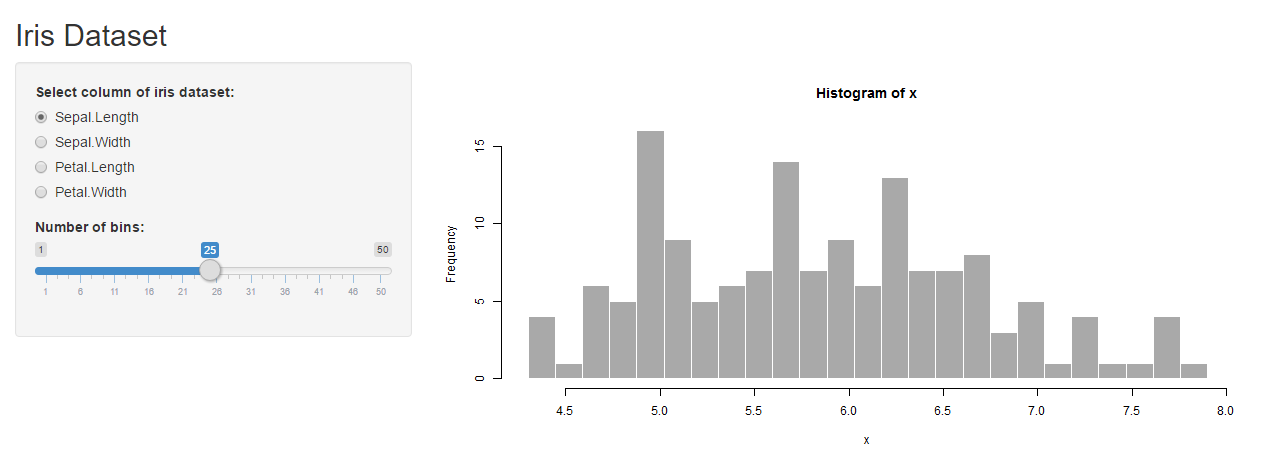
Example 4: Drawing histograms for iris dataset in R using Shiny
Creating Interactive data visualization using Shiny App in R (with examples)
1 | #UI.R |
1 | #SERVER.R |
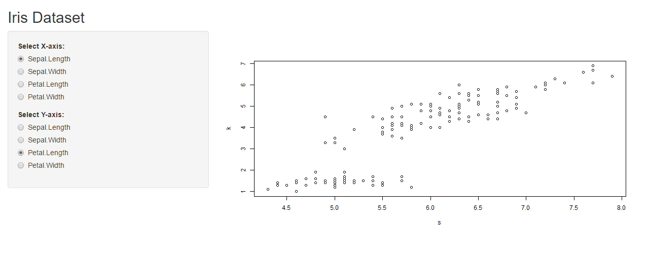
Example 5: Drawing Scatterplots for iris dataset in R using Shiny
Creating Interactive data visualization using Shiny App in R (with examples)
1 | #UI.R |
1 | #SERVER.R |
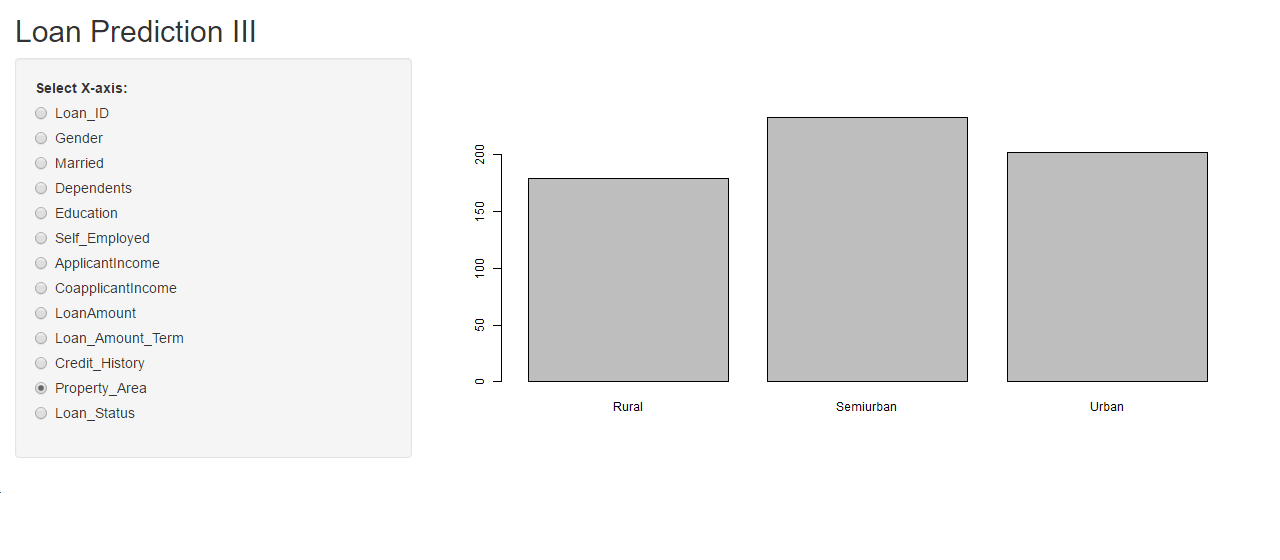
Example 6: Loan Prediction Practice problem
Creating Interactive data visualization using Shiny App in R (with examples)
To provide you hands on experience of creating shiny app, we will be using the Loan Prediction practice problem.
To brief you about the data set, the dataset we will be using is a Loan Prediction problem set in which Dream Housing Finance Company provides loans to customers based on their need. They want to automate the process of loan approval based on the personal details the customers provide like Gender, Marital Status, Education, Number of Dependents, Income, Loan Amount, Credit History and others.
- We will be creating an explanatory analysis of individual variables of the practice problem.
1 | #UI.R |
1 | #SERVER.R |
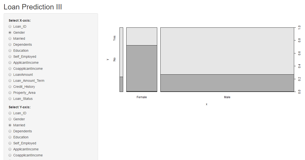
- Explanatory analysis of multiple variables of Loan Prediction Practice problem.
1 | #UI.R |
1 | #SERVER.R |
Advanced
Explore Shiny app with these add-on packages
Creating Interactive data visualization using Shiny App in R (with examples)
To add some more functionality to your Shiny App, there are some kick-ass packages available at your disposal. Here are few from RStudio.
- http://rstudio.github.io/shinythemes/
- http://rstudio.github.io/leaflet/
- https://rstudio.github.io/shinydashboard/
- http://shiny.rstudio.com/reference/shiny/latest/
Additional Resources
In the article I have covered the key areas of Shiny to help you get started with it. Personally to me Shiny is an interesting creation and to make the most of it, I think you should explore more. Here are few additional resources for you to become an adept in creating Shiny Apps.
- http://shiny.rstudio.com/tutorial/
- http://shiny.rstudio.com/images/shiny-cheatsheet.pdf
- http://shiny.rstudio.com/articles/
- http://www.showmeshiny.com/.
- http://www.shinyapps.io/
- http://shiny.rstudio.com/gallery/google-charts.html
- Shiny Google User Group
UI
sidebarPanel
A
actionButton
C
checkboxGroupInput
D
dateInput
dateRangeInput
F
fileInput
N
numericInput
P
passwordInput
R
radioButtons
S
selectInput
sliderInput
submitButton
T
textAreaInput
textInput
V
varSelectInput