AWS Machine Learning
Introduction
Machine learning for every data scientist and developer
AWS offers the broadest and deepest set of machine learning services and supporting cloud infrastructure, putting machine learning in the hands of every developer, data scientist and expert practitioner. AWS is helping more than one hundred thousand customers accelerate their machine learning journey.
Udacity
Course Overview
- Lesson 2: Introduction to Machine Learning – In this lesson, you will learn the fundamentals of supervised and unsupervised machine learning, including the process steps of solving machine learning problems, and explore several examples.
- Lesson 3: Machine Learning with AWS – In this lesson, you will learn about advanced machine learning techniques such as generative AI, reinforcement learning, and computer vision. You will also learn how to train these models with AWS AI/ML services.
- Lesson 4: Software Engineering Practices, part 1 – In this lesson, you will learn how to write well-documented, modularized code.
- Lesson 5: Software Engineering Practices, part 2 – In this lesson, you will learn how to test your code and log best practices.
- Lesson 6: Object-Oriented Programming – In this lesson, you will learn about this programming style and prepare to write your own Python package.
By the end of the course, you will be able to…
- Explain machine learning and the types of questions machine learning can help to solve.
- Explain what machine learning solutions AWS offers and how AWS AI devices put machine learning in the hands of every developer.
- Apply software engineering principles of modular code, code efficiency, refactoring, documentation, and version control to data science.
- Apply software engineering principles of testing code, logging, and conducting code reviews to data science.
Implement the basic principles of object-oriented programming to build a Python package.
Introduction to Machine Learning
Lesson Outline
Machine learning is creating rapid and exciting changes across all levels of society.
- It is the engine behind the recent advancements in industries such as autonomous vehicles.
- It allows for more accurate and rapid translation of the text into hundreds of languages.
- It powers the AI assistants you might find in your home.
- It can help improve worker safety.
- It can speed up drug design.
This lesson is divided into the following sections:
- First, we’ll discuss what machine learning is, common terminology, and common components involved in creating a machine learning project.
- Next, we’ll step into the shoes of a machine learning practitioner. Machine learning involves using trained models to generate predictions and detect patterns from data. To understand the process, we’ll break down the different steps involved and examine a common process that applies to the majority of machine learning projects.
- Finally, we’ll take you through three examples using the steps we described to solve real-life scenarios that might be faced by machine learning practitioners.
Learning Objectives
By the end of the Introduction to machine learning section, you will be able to do the following. Take a moment to read through these, checking off each item as you go through them.
Differentiate between supervised learning and unsupervised learning.
Identify problems that can be solved with machine learning.
Describe commonly used algorithms including linear regression, logistic regression, and k-means.
Describe how model training and testing works.
Evaluate the performance of a machine learning model using metrics.
What is Machine Learning?
Machine learning (ML) is a modern software development technique and a type of artificial intelligence (AI) that enables computers to solve problems by using examples of real-world data. It allows computers to automatically learn and improve from experience without being explicitly programmed to do so.
Summary
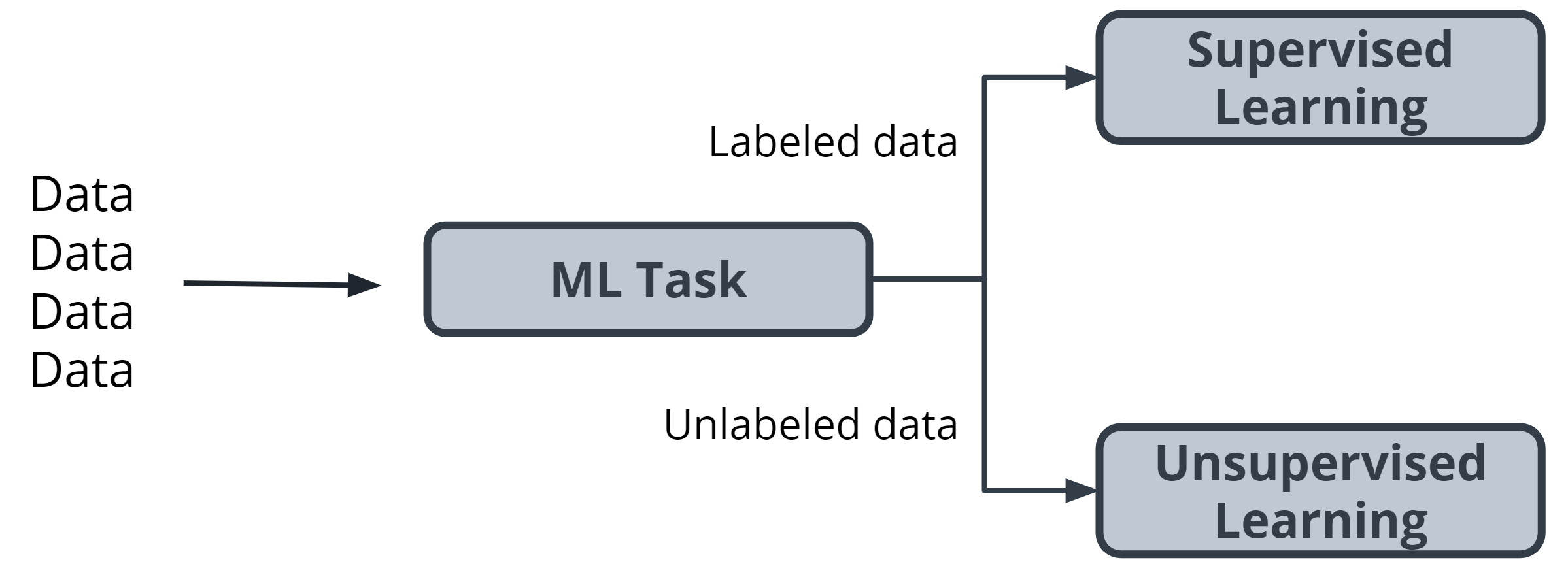
Machine learning is part of the broader field of artificial intelligence. This field is concerned with the capability of machines to perform activities using human-like intelligence. Within machine learning there are several different kinds of tasks or techniques:
- In supervised learning, every training sample from the dataset has a corresponding label or output value associated with it. As a result, the algorithm learns to predict labels or output values. We will explore this in-depth in this lesson.
- In unsupervised learning, there are no labels for the training data. A machine learning algorithm tries to learn the underlying patterns or distributions that govern the data. We will explore this in-depth in this lesson.
- In reinforcement learning, the algorithm figures out which actions to take in a situation to maximize a reward (in the form of a number) on the way to reaching a specific goal. This is a completely different approach than supervised and unsupervised learning. We will dive deep into this in the next lesson.
How does machine learning differ from traditional programming based approaches?
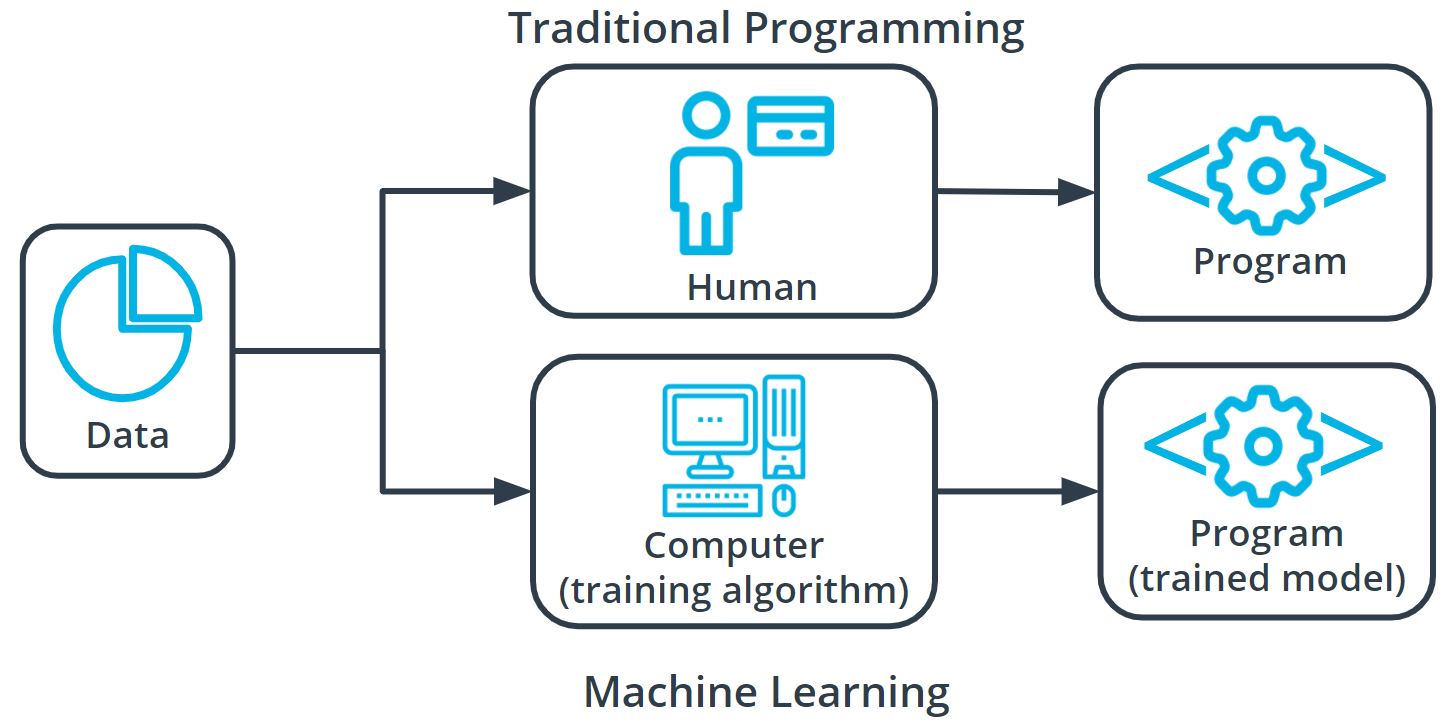
In traditional problem-solving with software, a person analyzes a problem and engineers a solution in code to solve that problem (image a bunch of if.. else conditions). For many real-world problems, this process can be laborious (or even impossible) because a correct solution would need to consider a vast number of edge cases.
Imagine, for example, the challenging task of writing a program that can detect if a cat is present in an image. Solving this in the traditional way would require careful attention to details like varying lighting conditions, different types of cats, and various poses a cat might be in.
In machine learning, the problem solver abstracts away part of their solution as a flexible component called a model, and uses a special program called a model training algorithm to adjust that model to real-world data. The result is a trained model which can be used to predict outcomes that are not part of the data set used to train it.
In a way, machine learning automates some of the statistical reasoning and pattern-matching the problem solver would traditionally do.
The overall goal is to use a model created by a model training algorithm to generate predictions or find patterns in data that can be used to solve a problem.
Understanding Terminology
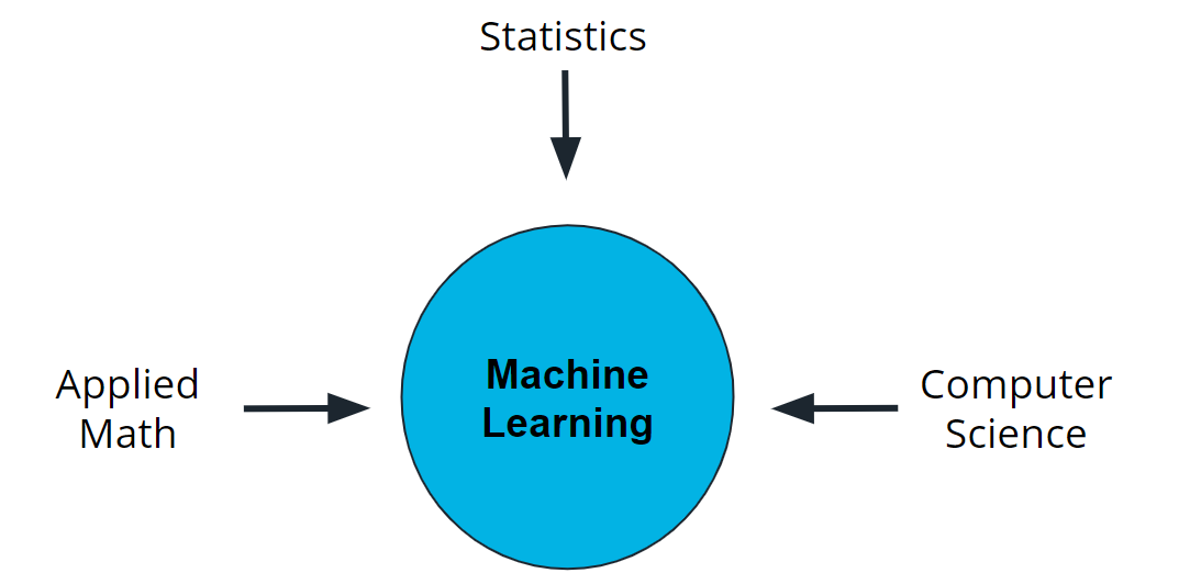
Machine learning is a new field created at the intersection of statistics, applied math, and computer science. Because of the rapid and recent growth of machine learning, each of these fields might use slightly different formal definitions of the same terms.
Terminology
Machine learning, or ML, is a modern software development technique that enables computers to solve problems by using examples of real-world data.
In supervised learning, every training sample from the dataset has a corresponding label or output value associated with it. As a result, the algorithm learns to predict labels or output values.
In reinforcement learning, the algorithm figures out which actions to take in a situation to maximize a reward (in the form of a number) on the way to reaching a specific goal.
In unsupervised learning, there are no labels for the training data. A machine learning algorithm tries to learn the underlying patterns or distributions that govern the data.
Additional Reading
- Want to learn more about how software and application come together? Reading through this entry about the software development process from Wikipedia can help.
Components of Machine Learning
Nearly all tasks solved with machine learning involve three primary components:
- A machine learning model
- A model training algorithm
- A model inference algorithm
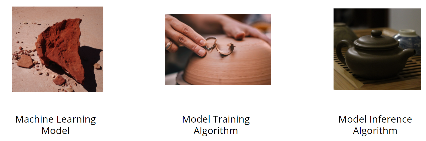
Clay Analogy for Machine Learning
You can understand the relationships between these components by imagining the stages of crafting a teapot from a lump of clay.
- First, you start with a block of raw clay. At this stage, the clay can be molded into many different forms and be used to serve many different purposes. You decide to use this lump of clay to make a teapot.
- So how do you create this teapot? You inspect and analyze the raw clay and decide how to change it to make it look more like the teapot you have in mind.
- Next, you mold the clay to make it look more like the teapot that is your goal.
Congratulations! You’ve completed your teapot. You’ve inspected the materials, evaluated how to change them to reach your goal, and made the changes, and the teapot is now ready for your enjoyment.
What are machine learning models?
A machine learning model, like a piece of clay, can be molded into many different forms and serve many different purposes. A more technical definition would be that a machine learning model is a block of code or framework that can be modified to solve different but related problems based on the data provided.
Important
- A model is an extremely generic program(or block of code), made specific by the data used to train it. It is used to solve different problems.
Two simple examples
Example 1
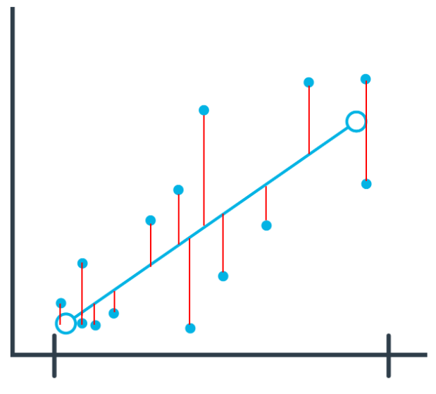
Imagine you own a snow cone cart, and you have some data about the average number of snow cones sold per day based on the high temperature. You want to better understand this relationship to make sure you have enough inventory on hand for those high sales days.
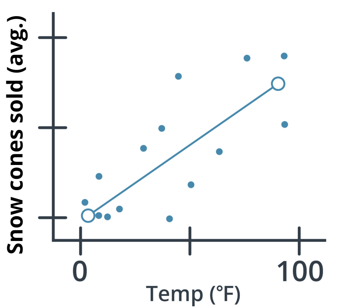
In the graph above, you can see one example of a model, a linear regression model (indicated by the solid line). You can see that, based on the data provided, the model predicts that as the high temperate for the day increases so do the average number of snow cones sold. Sweet!
Example 2
Let’s look at a different example that uses the same linear regression model, but with different data and to answer completely different questions.
Imagine that you work in higher education and you want to better understand the relationship between the cost of enrollment and the number of students attending college. In this example, our model predicts that as the cost of tuition increases the number of people attending college is likely to decrease.
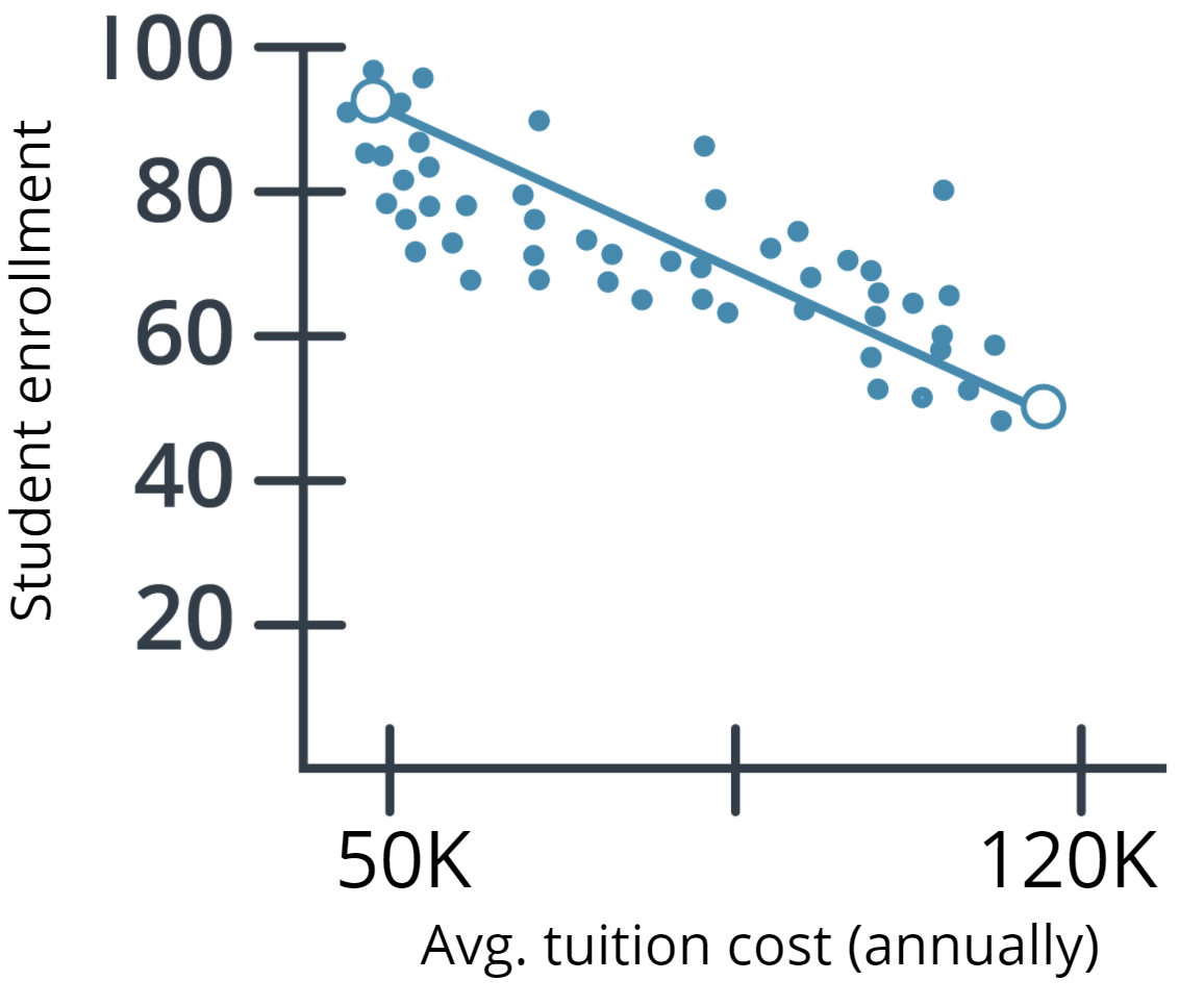
Using the same linear regression model (indicated by the solid line), you can see that the number of people attending college does go down as the cost increases.
Both examples showcase that a model is a generic program made specific by the data used to train it.
Model Training
How are model training algorithms used to train a model?
In the preceding section, we talked about two key pieces of information: a model and data. In this section, we show you how those two pieces of information are used to create a trained model. This process is called model training.
Model training algorithms work through an interactive process
Let’s revisit our clay teapot analogy. We’ve gotten our piece of clay, and now we want to make a teapot. Let’s look at the algorithm for molding clay and how it resembles a machine learning algorithm:
- Think about the changes that need to be made. The first thing you would do is inspect the raw clay and think about what changes can be made to make it look more like a teapot. Similarly, a model training algorithm uses the model to process data and then compares the results against some end goal, such as our clay teapot.
- Make those changes. Now, you mold the clay to make it look more like a teapot. Similarly, a model training algorithm gently nudges specific parts of the model in a direction that brings the model closer to achieving the goal.
- Repeat. By iterating over these steps over and over, you get closer and closer to what you want until you determine that you’re close enough that you can stop.


Model Inference: Using Your Trained Model
Now you have our completed teapot. You inspected the clay, evaluated the changes that needed to be made, and made them, and now the teapot is ready for you to use. Enjoy your tea!
So what does this mean from a machine learning perspective? We are ready to use the model inference algorithm to generate predictions using the trained model. This process is often referred to as model inference.

Terminology
A model is an extremely generic program, made specific by the data used to train it.
**Model training algorithms **work through an interactive process where the current model iteration is analyzed to determine what changes can be made to get closer to the goal. Those changes are made and the iteration continues until the model is evaluated to meet the goals.
Model inference is when the trained model is used to generate predictions.
Quiz: What is Machine Learning?
Think back to the clay teapot analogy. Is it true or false that you always need to have an idea of what you’re making when you’re handling your raw block of clay?
<span title=’Unsupervised learning uses unlabeled data and only works to find the patterns present in data, so you don’t always need to have a teapot in mind when you receive your raw block of clay.’> True
<span title=’You are correct that unsupervised learning uses unlabeled data and only works to find the patterns present in data, so you don’t always need to have a teapot in mind when you receive your raw block of clay.’> False
We introduced three common components of machine learning. Let’s review your new knowledge by matching each component to its definition.
| MACHINE LEARNING COMPONENT | DEFINITION |
|---|---|
| Machine learning model | Generic program, made specific by data |
| Model training algorithm | An iterative process fitting a generic model to specific data |
| Model inference algorithm | Process to use a rained model to sole a task |
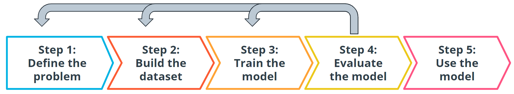
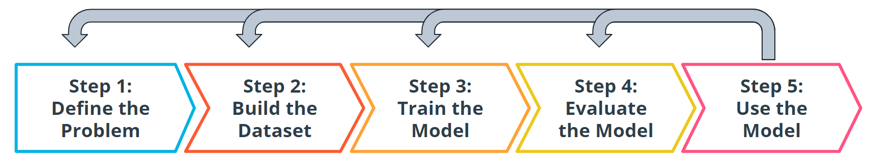
Introduction to the Five Machine Learning Steps
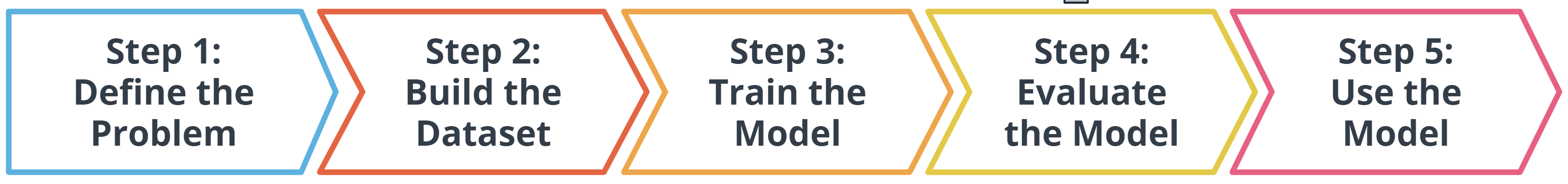
Major Steps in the Machine Learning Process
In the preceding diagram, you can see an outline of the major steps of the machine learning process. Regardless of the specific model or training algorithm used, machine learning practitioners practice a common workflow to accomplish machine learning tasks.
These steps are iterative. In practice, that means that at each step along the process, you review how the process is going. Are things operating as you expected? If not, go back and revisit your current step or previous steps to try and identify the breakdown.
Step 1: Define the Problem
How do You Start a Machine Learning Task?
- Define a very specific task.
- Think back to the snow cone sales example. Now imagine that you own a frozen treats store and you sell snow cones along with many other products. You wonder, “‘How do I increase sales?” It’s a valid question, but it’s the opposite of a very specific task. The following examples demonstrate how a machine learning practitioner might attempt to answer that question.
- “Does adding a $1.00 charge for sprinkles on a hot fudge sundae increase the sales of hot fudge sundaes?”
- “Does adding a $0.50 charge for organic flavors in your snow cone increase the sales of snow cones?”
- Think back to the snow cone sales example. Now imagine that you own a frozen treats store and you sell snow cones along with many other products. You wonder, “‘How do I increase sales?” It’s a valid question, but it’s the opposite of a very specific task. The following examples demonstrate how a machine learning practitioner might attempt to answer that question.
- Identify the machine learning task we might use to solve this problem.
- This helps you better understand the data you need for a project.
What is a Machine Learning Task?
All model training algorithms, and the models themselves, take data as their input. Their outputs can be very different and are classified into a few different groups based on the task they are designed to solve. Often, we use the kind of data required to train a model as part of defining a machine learning task.
In this lesson, we will focus on two common machine learning tasks:
- Supervised learning
- Unsupervised learning
Supervised and Unsupervised Learning
The presence or absence of labeling in your data is often used to identify a machine learning task.
Supervised tasks
A task is supervised if you are using labeled data. We use the term labeled to refer to data that already contains the solutions, called labels.
For example: Predicting the number of snow cones sold based on the temperatures is an example of supervised learning. In this example, the task is linear regression.
In the preceding graph, the data contains both a temperature and the number of snow cones sold. Both components are used to generate the linear regression shown on the graph. Our goal was to predict the number of snow cones sold, and we feed that value into the model. We are providing the model with labeled data and therefore, we are performing a supervised machine learning task.
Unsupervised tasks
A task is considered to be unsupervised if you are using unlabeled data. This means you don’t need to provide the model with any kind of label or solution while the model is being trained.
Let’s take a look at unlabeled data.


- Take a look at the preceding picture. Did you notice the tree in the picture? What you just did, when you noticed the object in the picture and identified it as a tree, is called labeling the picture. Unlike you, a computer just sees that image as a matrix of pixels of varying intensity.
- Since this image does not have the labeling in its original data, it is considered unlabeled.
How do we classify tasks when we don’t have a label?
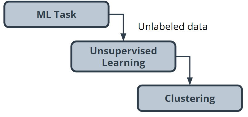
Unsupervised learning involves using data that doesn’t have a label. One common task is called clustering. Clustering helps to determine if there are any naturally occurring groupings in the data.
Let’s look at an example of how clustering in unlabeled data works.
Identifying book micro-genres with unsupervised learning
Imagine that you work for a company that recommends books to readers.
The assumption: You are fairly confident that micro-genres exist, and that there is one called Teen Vampire Romance. Because you don’t know which micro-genres exist, you can’t use supervised learning techniques.
This is where the unsupervised learning clustering technique might be able to detect some groupings in the data. The words and phrases used in the book description might provide some guidance on a book’s micro-genre.
Further Classifying by using Label Types
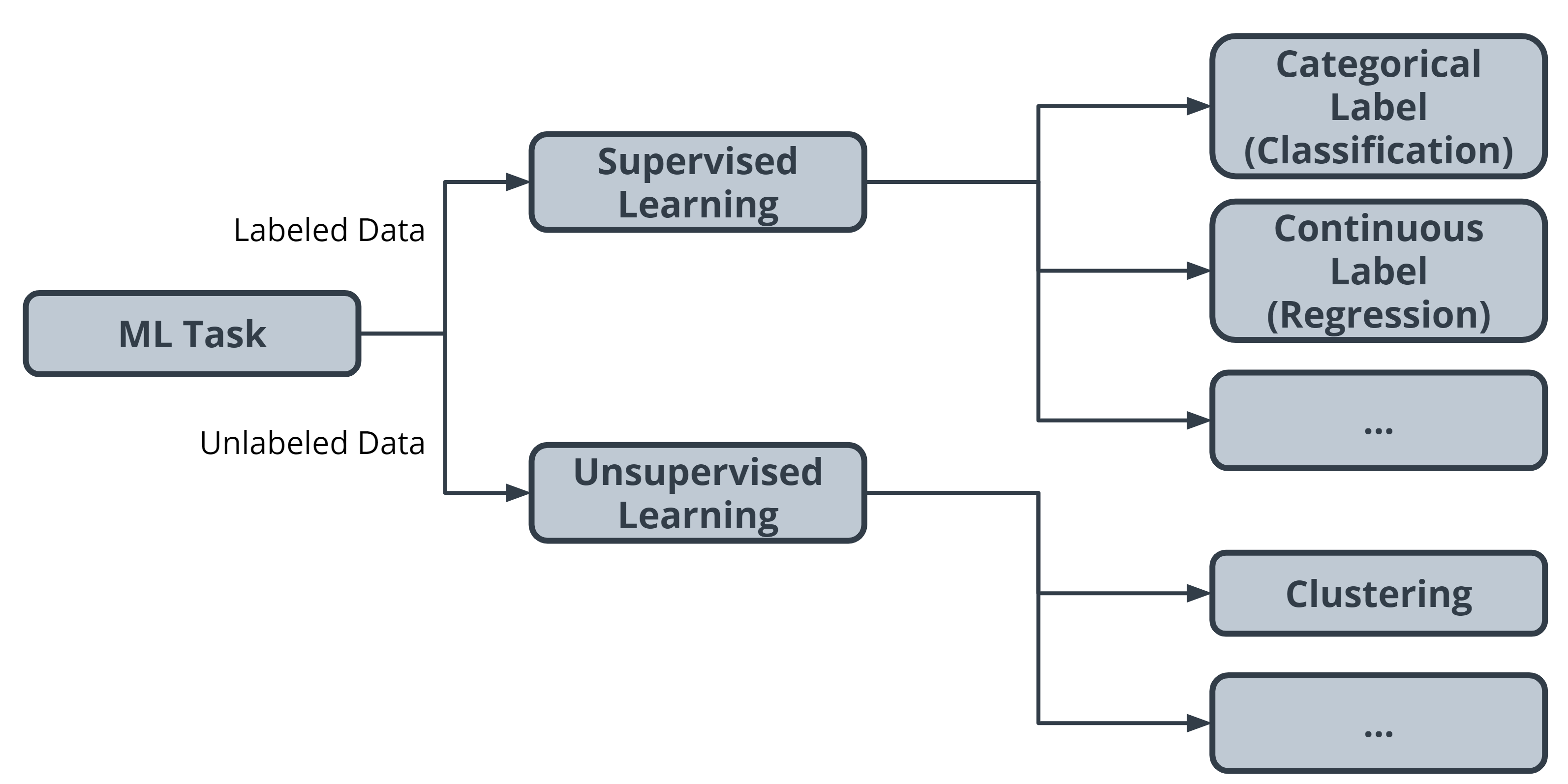
Initially, we divided tasks based on the presence or absence of labeled data while training our model. Often, tasks are further defined by the type of label which is present.
In supervised learning, there are two main identifiers you will see in machine learning:
- A categorical label has a discrete set of possible values. In a machine learning problem in which you want to identify the type of flower based on a picture, you would train your model using images that have been labeled with the categories of flower you would want to identify. Furthermore, when you work with categorical labels, you often carry out classification tasks, which are part of the supervised learning family.
- A continuous (regression) label does not have a discrete set of possible values, which often means you are working with numerical data. In the snow cone sales example, we are trying to predict the number of snow cones sold. Here, our label is a number that could, in theory, be any value.
In unsupervised learning, clustering is just one example. There are many other options, such as deep learning.
Terminology
- Clustering. Unsupervised learning task that helps to determine if there are any naturally occurring groupings in the data.
- A categorical label has a discrete set of possible values, such as “is a cat” and “is not a cat.”
- A continuous (regression) label does not have a discrete set of possible values, which means possibly an unlimited number of possibilities.
- Discrete: A term taken from statistics referring to an outcome taking on only a finite number of values (such as days of the week).
- A label refers to data that already contains the solution.
- Using unlabeled data means you don’t need to provide the model with any kind of label or solution while the model is being trained.
Additional Reading
- The AWS Machine Learning blog is a great resource for learning more about projects in machine learning.
- You can use Amazon SageMaker to calculate new stats in Major League Baseball.
- You can also find an article on Flagging suspicious healthcare claims with Amazon SageMaker on the AWS Machine Learning blog.
- What kinds of questions and problems are good for machine learning?
You can use supervised ML approaches for these specific machine learning tasks: binary classification (predicting one of two possible outcomes), multiclass classification (predicting one of more than two outcomes) and regression (predicting a numeric value).
Examples of binary classification problems:
- Will the customer buy this product or not buy this product?
- Is this email spam or not spam?
- Is this product a book or a farm animal?
- Is this review written by a customer or a robot?
Examples of multiclass classification problems:
- Is this product a book, movie, or clothing?
- Is this movie a romantic comedy, documentary, or thriller?
- Which category of products is most interesting to this customer?
Examples of regression classification problems:
- What will the temperature be in Seattle tomorrow?
- For this product, how many units will sell?
- How many days before this customer stops using the application?
- What price will this house sell for?
Quiz 1
Which of the following problem statements fit the definition of a regression-based task?
I want to detect when my cat jumps on the dinner table, so I set up a camera and write a program to determine if my cat is in the frame or not in the frame.
I want to determine the expected reading time for online news articles, so I collect data on my reading time for a week and write a browser plugin to use that data to predict the reading time for new articles.
I believe my customers fall into one of many customer segments, but I don’t know what those segments are in advance. After asking for permission, I collect a bunch of data on their actions when they use my product and try to determine if there are many collections of users that behave in similar ways.
I work for a shoe company and want to provide a service to help parents predict their children’s shoe size for any particular age. Within this system, I represent shoe size as a continuum of values and then round to the nearest shoe size.
Both answers chosen here involve trying to predict some unknown continuous attribute about your data.
Remember: Classification tasks involve predicting some unknown categorical attribute about your data.
Regression tasks involve predicting some unknown continuous attribute about your data.
Clustering tasks involve exploring how your data might be grouped together.
As a machine learning practitioner, you’re working with stakeholders on a music streaming app. Your supervisor asks, “How can we increase the average number of minutes a customer spends listening on our app?”
This is a broad question(too broad) with many different potential factors affecting how long a customer might spend listening to music.
How might you change the scope or redefine the question to be better suited, and more concise, for a machine learning task?
Will changing the frequency of when we start playing ad affect how long a customer listens to music on our service?
Will creating custom playlists encourage customers to listen to music longer?
Will creating artist interviews about their songs increase how long our customers spend listening to music?
Step 2: Build a Dataset
Summary
The next step in the machine learning process is to build a dataset that can be used to solve your machine learning-based problem. Understanding the data needed helps you select better models and algorithms so you can build more effective solutions.
The most important step of the machine learning process
Working with data is perhaps the most overlooked—yet most important—step of the machine learning process. In 2017, an O’Reilly study showed that machine learning practitioners spend 80% of their time working with their data.
The Four Aspects of Working with Data
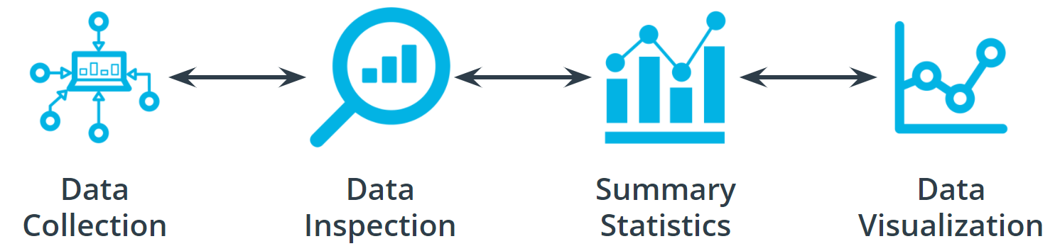
You can take an entire class just on working with, understanding, and processing data for machine learning applications. Good, high-quality data is essential for any kind of machine learning project. Let’s explore some of the common aspects of working with data.
Data collection
Data collection can be as straightforward as running the appropriate SQL queries or as complicated as building custom web scraper applications to collect data for your project. You might even have to run a model over your data to generate needed labels. Here is the fundamental question:
Does the data you’ve collected match the machine learning task and problem you have defined?
Data inspection
The quality of your data will ultimately be the largest factor that affects how well you can expect your model to perform. As you inspect your data, look for:
- Outliers
- Missing or incomplete values
- Data that needs to be transformed or preprocessed so it’s in the correct format to be used by your model
Summary statistics
Models can assume how your data is structured.
Now that you have some data in hand it is a good best practice to check that your data is in line with the underlying assumptions of your chosen machine learning model.
With many statistical tools, you can calculate things like the mean, inner-quartile range (IQR), and standard deviation. These tools can give you insight into the scope, scale, and shape of the dataset.
Data visualization
You can use data visualization to see outliers and trends in your data and to help stakeholders understand your data.
Look at the following two graphs. In the first graph, some data seems to have clustered into different groups. In the second graph, some data points might be outliers.


Terminology
- Impute is a common term referring to different statistical tools which can be used to calculate missing values from your dataset.
- Outliers are data points that are significantly different from others in the same sample.
Additional reading
- In machine learning, you use several statistical-based tools to better understand your data. The
sklearnlibrary has many examples and tutorials, such as this example demonstrating outlier detection on a real dataset.
Quiz 2
True or false: Your data requirements will not change based on the machine learning task you are using.
True
False
True or false: Models are universal, so the data is not relevant.
True
False
True or false: Data needs to be formatted so that is compatible with the model and model training algorithm you plan to use.
True
False
True or false: Data visualizations are the only way to identify outliers in your data.
True
False
True or false: After you start using your model (performing inference), you don’t need to check the new data that it receives.
True
False
Step 3: Model Training
1. Splitting your Dataset
The first step in model training is to randomly split the dataset. This allows you to keep some data hidden during training, so that data can be used to evaluate your model before you put it into production. Specifically, you do this to test against the bias-variance trade-off. If you’re interested in learning more, see the Further learning and reading section.
Splitting your dataset gives you two sets of data:
- Training dataset: The data on which the model will be trained. Most of your data will be here. Many developers estimate about 80%.
- Test dataset: The data withheld from the model during training, which is used to test how well your model will generalize to new data.
1 | X, y = ckd.drop(['Class'], axis=1), df['Class'] |
1 | from sklearn.model_selection import train_test_split |
Model Training Terminology
The model training algorithm iteratively updates a model’s parameters to minimize some loss function.
Let’s define those two terms:
- Model parameters: Model parameters are settings or configurations the training algorithm can update to change how the model behaves. Depending on the context, you’ll also hear other more specific terms used to describe model parameters such as weights and biases. Weights, which are values that change as the model learns, are more specific to neural networks.
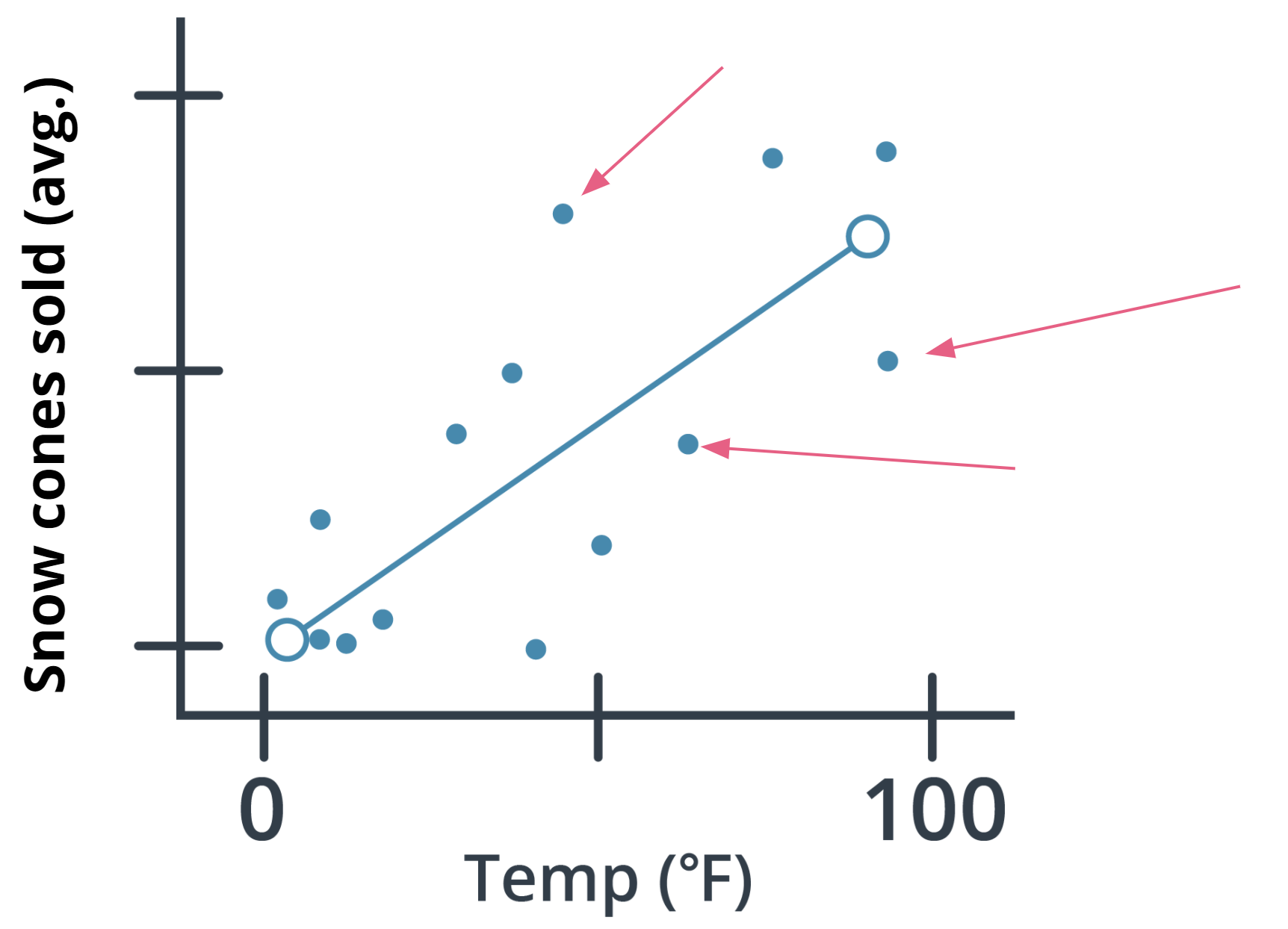
- Loss function: A loss function is used to codify the model’s distance from this goal. For example, if you were trying to predict a number of snow cone sales based on the day’s weather, you would care about making predictions that are as accurate as possible. So you might define a loss function to be “the average distance between your model’s predicted number of snow cone sales and the correct number.” You can see in the snow cone example this is the difference between the two purple dots.
Putting it All Together
The end-to-end training process is
- Feed the training data into the model.
- Compute the loss function on the results.
- Update the model parameters in a direction that reduces loss.
You continue to cycle through these steps until you reach a predefined stop condition. This might be based on a training time, the number of training cycles, or an even more intelligent or application-aware mechanism.
Advice From the Experts
Remember the following advice when training your model.
- Practitioners often use machine learning frameworks that already have working implementations of models and model training algorithms. You could implement these from scratch, but you probably won’t need to do so unless you’re developing new models or algorithms.
- Practitioners use a process called model selection to determine which model or models to use. The list of established models is constantly growing, and even seasoned machine learning practitioners may try many different types of models while solving a problem with machine learning.
- Hyperparameters are settings on the model which are not changed during training but can affect how quickly or how reliably the model trains, such as the number of clusters the model should identify.
- Be prepared to iterate.
Pragmatic problem solving with machine learning is rarely an exact science, and you might have assumptions about your data or problem which turn out to be false. Don’t get discouraged. Instead, foster a habit of trying new things, measuring success, and comparing results across iterations.
Extended Learning
This information hasn’t been covered in the above video but is provided for the advanced reader.
Linear models
One of the most common models covered in introductory coursework, linear models simply describe the relationship between a set of input numbers and a set of output numbers through a linear function (think of $y = mx + b$ or a line on a $x$ vs $y$ chart).
Classification tasks often use a strongly related logistic model, which adds an additional transformation mapping the output of the linear function to the range [0, 1] (correlation coefficient), interpreted as “probability of being in the target class.” Linear models are fast to train and give you a great baseline against which to compare more complex models. A lot of media buzz is given to more complex models, but for most new problems, consider starting with a simple model.
Tree-based models
Tree-based models are probably the second most common model type covered in introductory coursework. They learn to categorize or regress by building an extremely large structure of nested if/else blocks, splitting the world into different regions at each if/else block. Training determines exactly where these splits happen and what value is assigned at each leaf region.
For example, if you’re trying to determine if a light sensor is in sunlight or shadow, you might train tree of depth 1 with the final learned configuration being something like if (sensor_value > 0.698), then return 1; else return 0;. The tree-based model XGBoost is commonly used as an off-the-shelf implementation for this kind of model and includes enhancements beyond what is discussed here. Try tree-based models to quickly get a baseline before moving on to more complex models.
Deep learning models
Extremely popular and powerful, deep learning is a modern approach based around a conceptual model of how the human brain functions. The model (also called a neural network) is composed of collections of neurons (very simple computational units) connected together by weights (mathematical representations of how much information to allow to flow from one neuron to the next). The process of training involves finding values for each weight.
Various neural network structures have been determined for modeling different kinds of problems or processing different kinds of data.
A short (but not complete!) list of noteworthy examples includes:
- FFNN: The most straightforward way of structuring a neural network, the Feed Forward Neural Network (FFNN) structures neurons in a series of layers, with each neuron in a layer containing weights to all neurons in the previous layer.
- CNN: Convolutional Neural Networks (CNN) represent nested filters over grid-organized data. They are by far the most commonly used type of model when processing images.
- RNN/LSTM: Recurrent Neural Networks (RNN) and the related Long Short-Term Memory (LSTM) model types are structured to effectively represent for loops in traditional computing, collecting state while iterating over some object. They can be used for processing sequences of data.
- Transformer: A more modern replacement for RNN/LSTMs, the transformer architecture enables training over larger datasets involving sequences of data.
Machine Learning Using Python Libraries
- For more classical models (linear, tree-based) as well as a set of common ML-related tools, take a look at
scikit-learn. The web documentation for this library is also organized for those getting familiar with space and can be a great place to get familiar with some extremely useful tools and techniques. - For deep learning,
mxnet,tensorflow, andpytorchare the three most common libraries. For the purposes of the majority of machine learning needs, each of these is feature-paired and equivalent.
Terminology
- Hyperparameters are settings on the model which are not changed during training but can affect how quickly or how reliably the model trains, such as the number of clusters the model should identify.
- A loss function is used to codify the model’s distance from this goal
- Training dataset: The data on which the model will be trained. Most of your data will be here.
- Test dataset: The data withheld from the model during training, which is used to test how well your model will generalize to new data.
- Model parameters are settings or configurations the training algorithm can update to change how the model behaves.
Additional reading
- The Wikipedia entry on the bias-variance trade-off can help you understand more about this common machine learning concept.
- In this AWS Machine Learning blog post, you can see how to train a machine-learning algorithm to predict the impact of weather on air quality using Amazon SageMaker.
Quiz 3
True or false: The loss function measures how far the model is from its goal.
True
False
Why do you need to split the data into training and test data prior to beginning model training?
It is a requirement of supervised learning tasks.
If you use all the data you have collected during training, you won’t have any with which to test the model during the model evaluation phase.
Any regression-based task requires splitting the data.
Any classification-based task requires splitting the data.
What makes hyperparameters different than model parameters? There may be more than one correct answer.
Hyperparameters are updated during model training.
Hyperparameters are not updated during model training.
Hyperparameters are set manually.
Hyperparameters are not set manually.
Step 4: Model Evaluation
After you have collected your data and trained a model, you can start to evaluate how well your model is performing. The metrics used for evaluation are likely to be very specific to the problem you have defined. As you grow in your understanding of machine learning, you will be able to explore a wide variety of metrics that can enable you to evaluate effectively.
Using Model Accuracy
Model accuracy is a fairly common evaluation metric. Accuracy is the fraction of predictions a model gets right.
Here’s an example:

Imagine that you built a model to identify a flower as one of two common species based on measurable details like petal length. You want to know how often your model predicts the correct species. This would require you to look at your model’s accuracy.
Extended Learning
This information hasn’t been covered in the above video but is provided for the advanced reader.
Using Log Loss
Log loss seeks to calculate how uncertain your model is about the predictions it is generating. In this context, uncertainty refers to how likely a model thinks the predictions being generated are to be correct.

For example, let’s say you’re trying to predict how likely a customer is to buy either a jacket or t-shirt.
Log loss could be used to understand your model’s uncertainty about a given prediction. In a single instance, your model could predict with 5% certainty that a customer is going to buy a t-shirt. In another instance, your model could predict with 80% certainty that a customer is going to buy a t-shirt. Log loss enables you to measure how strongly the model believes that its prediction is accurate.
In both cases, the model predicts that a customer will buy a t-shirt, but the model’s certainty about that prediction can change.
Remember: This Process is Iterative
Every step we have gone through is highly iterative and can be changed or re-scoped during the course of a project. At each step, you might find that you need to go back and reevaluate some assumptions you had in previous steps. Don’t worry! This ambiguity is normal.
Terminology
- Log loss seeks to calculate how uncertain your model is about the predictions it is generating.
- Model Accuracy is the fraction of predictions a model gets right.
Additional reading
The tools used for model evaluation are often tailored to a specific use case, so it’s difficult to generalize rules for choosing them. The following articles provide use cases and examples of specific metrics in use.
- This healthcare-based example, which automates the prediction of spinal pathology conditions, demonstrates how important it is to avoid false positive and false negative predictions using the tree-based
xgboostmodel. - The popular open-source library
sklearnprovides information about common metrics and how to use them. - This entry from the AWS Machine Learning blog demonstrates the importance of choosing the correct model evaluation metrics for making accurate energy consumption estimates using Amazon Forecast.
Quiz 4
True or false: Model evaluation is not very use case–specific.
True
False
Thinking deeper about linear regression
This lesson has covered linear regression in detail, explaining how you can envision minimizing loss, how the model can be used in various scenarios, and the importance of data.
What are some methods or tools that could be useful to consider when evaluating a linear regression output? Can you provide an example of a situation in which you would apply that method or tool?
In my experience, to perform a linear regression, there are several important steps for minimizing loss (Python):
- Data Inspection. Use pandas.DataFrame to check the quality of the dataset and determine how to deal with the missing values.
- Summary Statistics. Use pandas.DataFrame to see the mean, median, scale, or other metrics of the dataset.
- Standardization. For most scenarios, we need to standardize or normalized the dataset.
- Data Visualization. Use plotly to visualize the dataset. We can see the pattern, distribution, and outliers of the dataset. In this step, we can make a decision that which attributes should we use for Machine Learning. For Linear Regression, pandas has a great method .corr() for quickly checking the correlations between every two attributes.
- Perform Linear Regression. Validate the Accuracy in different combinations of attributes.
There are many different tools that can be used to evaluate a linear regression model. Here are a few examples:
The Method of Least Squares
Mean absolute error (MAE): This is measured by taking the average of the absolute difference between the actual values and the predictions. Ideally, this difference is minimal.
Root mean square error (RMSE): This is similar MAE, but takes a slightly modified approach so values with large error receive a higher penalty. RMSE takes the square root of the average squared difference between the prediction and the actual value.
Coefficient of determination or R-squared (R^2): This measures how well-observed outcomes are actually predicted by the model, based on the proportion of total variation of outcomes.
Step 5: Model Inference
Summary
Congratulations! You’re ready to deploy your model.
Once you have trained your model, have evaluated its effectiveness, and are satisfied with the results, you’re ready to generate predictions on real-world problems using unseen data in the field. In machine learning, this process is often called inference.
Iterative Process
Even after you deploy your model, you’re always monitoring to make sure your model is producing the kinds of results that you expect. There may be times where you reinvestigate the data, modify some of the parameters in your model training algorithm, or even change the model type used for training.
Quiz 5
Choose the options which correctly complete the following phrase:
Model inference involves…
Generating predictions
Finding patterns in your data
Using a trained model
Testing your model on data it has not seen before
Introduction to Examples
Through the remainder of the lesson, we will be walking through 3 different case study examples of machine learning tasks actually solving problems in the real world.
Supervised learning
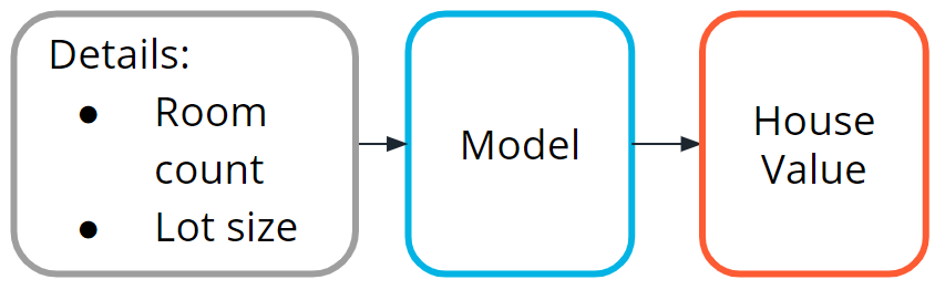
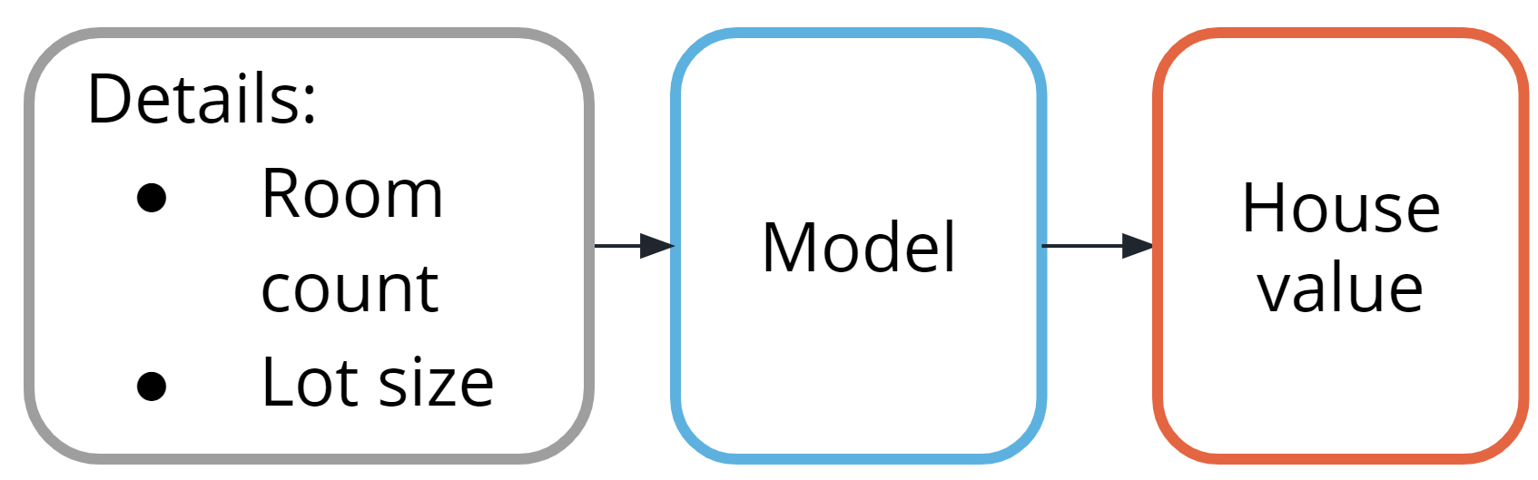
- Using machine learning to predict housing prices in a neighborhood based on lot size and number of bedrooms
Unsupervised learning
- Using machine learning to isolate micro-genres of books by analyzing the wording on the back cover description.
Deep neural network
- While this type of task is beyond the scope of this lesson, we wanted to show you the power and versatility of modern machine learning. You will see how it can be used to analyze raw images from lab video footage from security cameras, trying to detect chemical spills.
Example One: House Price Prediction
House price prediction is one of the most common examples used to introduce machine learning.
Traditionally, real estate appraisers use many quantifiable details about a home (such as number of rooms, lot size, and year of construction) to help them estimate the value of a house.
You detect this relationship and believe that you could use machine learning to predict home prices.
Step One: Define the Problem
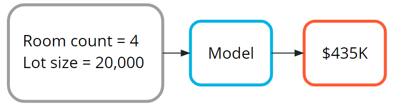
Can we estimate the price of a house based on lot size or the number of bedrooms?
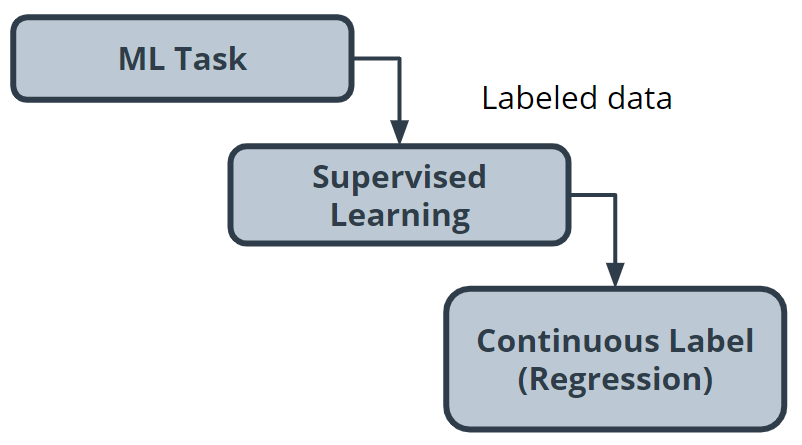
You access the sale prices for recently sold homes or have them appraised. Since you have this data, this is a supervised learning task. You want to predict a continuous numeric value, so this task is also a regression task.
Step Two: Building a Dataset
- Data collection: You collect numerous examples of homes sold in your neighborhood within the past year, and pay a real estate appraiser to appraise the homes whose selling price is not known.
- Data exploration: You confirm that all of your data is numerical because most machine learning models operate on sequences of numbers. If there is textual data, you need to transform it into numbers. You’ll see this in the next example.
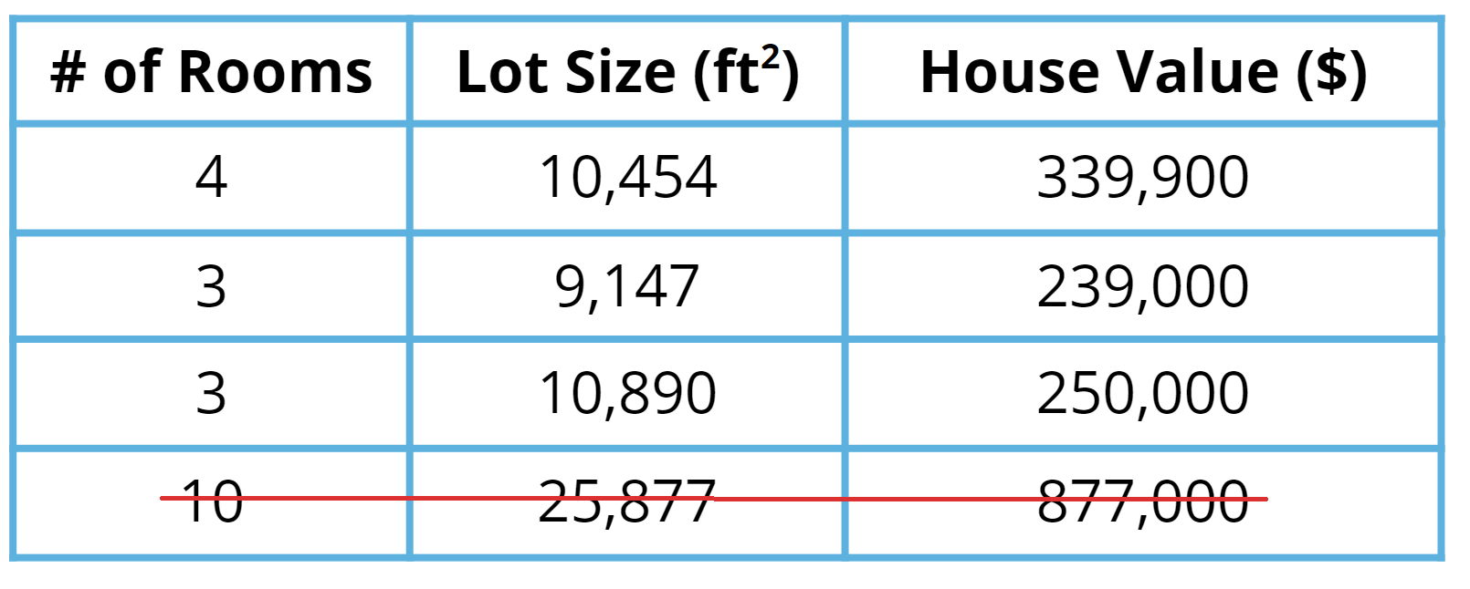
- Data cleaning: Look for things such as missing information or outliers, such as the 10-room mansion. Several techniques can be used to handle outliers, but you can also just remove those from your dataset.
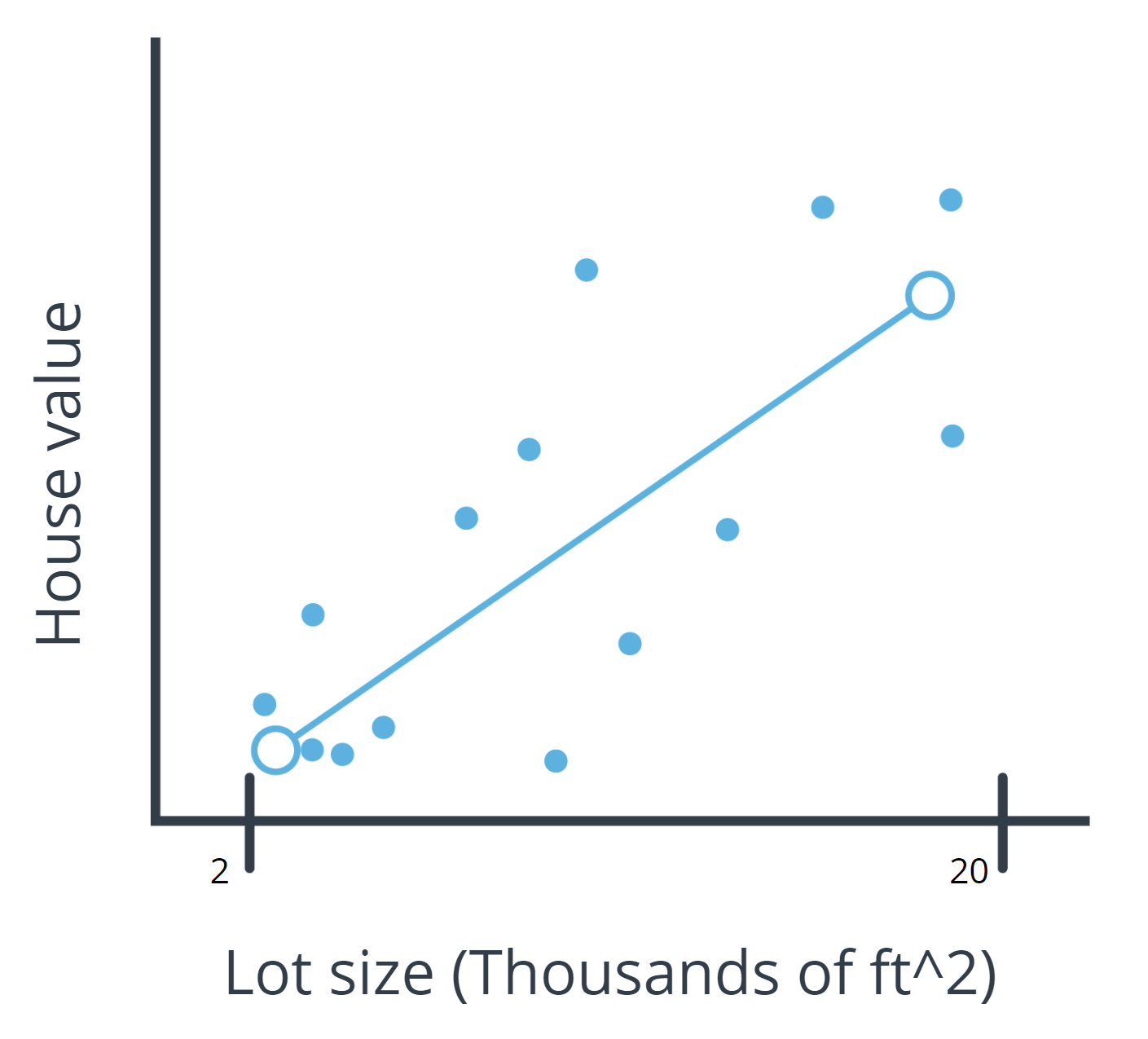
- Data visualization: You can plot home values against each of your input variables to look for trends in your data. In the following chart, you see that when lot size increases, the house value increases.
Step Three: Model Training
Prior to actually training your model, you need to split your data. The standard practice is to put 80% of your dataset into a training dataset and 20% into a test dataset.
Linear model selection
As you see in the preceding chart, when lot size increases, home values increase too. This relationship is simple enough that a linear model can be used to represent this relationship.
A linear model across a single input variable can be represented as a line. It becomes a plane for two variables, and then a hyperplane for more than two variables. The intuition, as a line with a constant slope, doesn’t change.
Using a Python library
The Python scikit-learn library has tools that can handle the implementation of the model training algorithm for you.
Step Four: Evaluation
One of the most common evaluation metrics in a regression scenario is called root mean square or RMS. The math is beyond the scope of this lesson, but RMS can be thought of roughly as the “average error” across your test dataset, so you want this value to be low.
$$\displaystyle RMS = \sqrt{\frac{1}{n}\sum_i{x_i^2}}$$
In the following chart, you can see where the data points are in relation to the blue line. You want the data points to be as close to the “average” line as possible, which would mean less net error.
You compute the root mean square between your model’s prediction for a data point in your test dataset and the true value from your data. This actual calculation is beyond the scope of this lesson, but it’s good to understand the process at a high level.
Interpreting Results
In general, as your model improves, you see a better RMS result. You may still not be confident about whether the specific value you’ve computed is good or bad.
Many machine learning engineers manually count how many predictions were off by a threshold (for example, $50,000 in this house pricing problem) to help determine and verify the model’s accuracy.
Step Five: Inference: Try out your model
Now you are ready to put your model into action. As you can see in the following image, this means seeing how well it predicts with new data not seen during model training.
Terminology
- Continuous: Floating-point values with an infinite range of possible values. The opposite of categorical or discrete values, which take on a limited number of possible values.
- Hyperplane: A mathematical term for a surface that contains more than two planes.
- Plane: A mathematical term for a flat surface (like a piece of paper) on which two points can be joined by a straight line.
- Regression: A common task in supervised machine learning.
Additional reading
The Machine Learning Mastery blog is a fantastic resource for learning more about machine learning. The following example blog posts dive deeper into training regression-based machine learning models.
- How to Develop Ridge Regression Models in Python offers another approach to solving the problem in the example from this lesson.
- Regression is a popular machine learning task, and you can use several different model evaluation metrics with it.
Quiz: Example One
True or False: The model used in this example is an unsupervised machine learning task.
True
False
In this example, we used a linear model to solve a simple regression supervised learning task. This model type is a great first choice when exploring a machine learning problem because it’s very fast and straightforward to train. It typically works well when you have relationships in your data that are linear (when input changes by X, output changes by some fixed multiple of X).
Can you think of an example of a problem that would not be solvable by a linear model?
Linear models typically fail when there is no helpful linear relationship between the input variables and the label.
For example, imagine predicting the height (label) of a thrown projectile over time (input variable). You know the trajectory is not linear; it’s curved. Any straight line you try to use to describe this phenomenon would be invalid for a large range of the projectile’s trajectory.
Techniques do exist to modify your data so you can still use linear models in these situations. Such methods are out of scope for this course but are called kernel methods.
Example Two: Book Genre Exploration
In this video, you saw how the machine learning process can be applied to an unsupervised machine learning task that uses book description text to identify different micro-genres.
Step One: Define the Problem
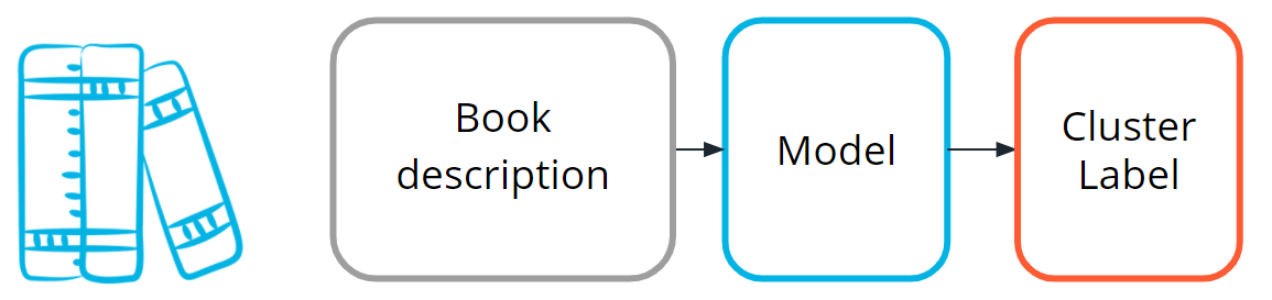
Find clusters of similar books based on the presence of common words in the book descriptions.
You do editorial work for a book recommendation company, and you want to write an article on the largest book trends of the year. You believe that a trend called “micro-genres” exists, and you have confidence that you can use the book description text to identify these micro-genres.
By using an unsupervised machine learning technique called clustering, you can test your hypothesis that the book description text can be used to identify these “hidden” micro-genres.
Earlier in this lesson, you were introduced to the idea of unsupervised learning. This machine learning task is especially useful when your data is not labeled.
Step Two: Build your Dataset
To test the hypothesis, you gather book description text for 800 romance books published in the current year.
Data exploration, cleaning and preprocessing
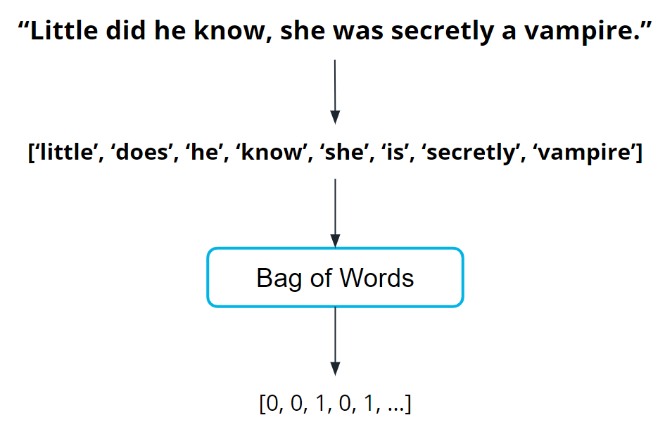
For this project, you believe capitalization and verb tense will not matter, and therefore you remove capitals and convert all verbs to the same tense using a Python library built for processing human language. You also remove punctuation and words you don’t think have useful meaning, like ‘a‘ and ‘the‘. The machine learning community refers to these words as stop words.
Before you can train the model, you need to do some data preprocessing, called data vectorization, to convert text into numbers.
You transform this book description text into what is called a bag of words representation shown in the following image so that it is understandable by machine learning models.
How the bag of words representation works is beyond the scope of this course. If you are interested in learning more, see the Additional Reading section at the bottom of the page.
Step Three: Train the Model
Now you are ready to train your model.
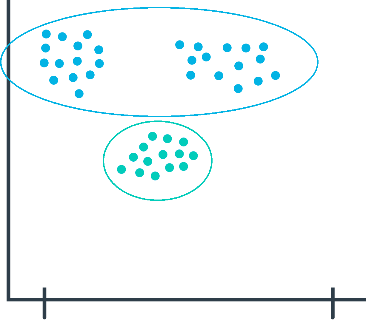
You pick a common cluster-finding model called k-means. In this model, you can change a model parameter, k, to be equal to how many clusters the model will try to find in your dataset.
Your data is unlabeled: you don’t how many microgenres might exist. So you train your model multiple times using different values for k each time.
What does this even mean? In the following graphs, you can see examples of when k=2 and when k=3.
During the model evaluation phase, you plan on using a metric to find which value for k is most appropriate.
Step Four: Model Evaluation
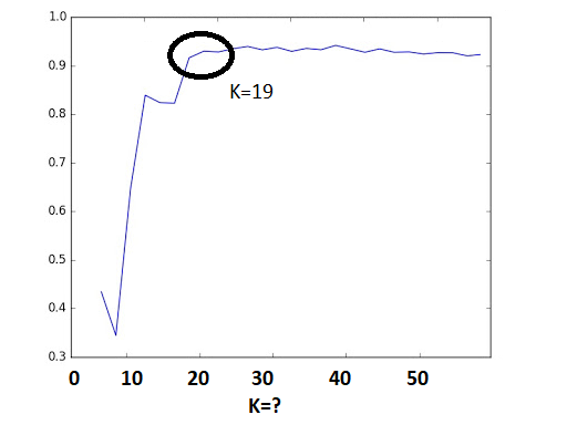
In machine learning, numerous statistical metrics or methods are available to evaluate a model. In this use case, the silhouette coefficient is a good choice. This metric describes how well your data was clustered by the model. To find the optimal number of clusters, you plot the silhouette coefficient as shown in the following image below. You find the optimal value is when k=19.
Often, machine learning practitioners do a manual evaluation of the model’s findings.
You find one cluster that contains a large collection of books you can categorize as “paranormal teen romance.” This trend is known in your industry, and therefore you feel somewhat confident in your machine learning approach. You don’t know if every cluster is going to be as cohesive as this, but you decide to use this model to see if you can find anything interesting about which to write an article.
Step Five: Inference (Use the Model)
As you inspect the different clusters found when k=19, you find a surprisingly large cluster of books. Here’s an example from fictionalized cluster #7.
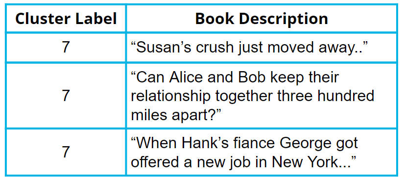
As you inspect the preceding table, you can see that most of these text snippets are indicating that the characters are in some kind of long-distance relationship. You see a few other self-consistent clusters and feel you now have enough useful data to begin writing an article on unexpected modern romance microgenres.
Terminology
- Bag of words: A technique used to extract features from the text. It counts how many times a word appears in a document (corpus), and then transforms that information into a dataset.
- Data vectorization: A process that converts non-numeric data into a numerical format so that it can be used by a machine learning model.
- Silhouette coefficient: A score from
-1to1describing the clusters found during modeling. A score near zero indicates overlapping clusters, and scores less than zero indicate data points assigned to incorrect clusters. A score approaching 1 indicates successful identification of discrete non-overlapping clusters. - Stop words: A list of words removed by natural language processing tools when building your dataset. There is no single universal list of stop words used by all-natural language processing tools.
Additional reading
Machine Learning Mastery is a great resource for finding examples of machine learning projects.
- The How to Develop a Deep Learning Bag-of-Words Model for Sentiment Analysis (Text Classification) blog post provides an example using a bag of words–based approach pair with a deep learning model.
Quiz: Example Two
What kind of machine learning task was used in the book micro-genre example?
Supervised Learning
Unsupervised Learning
In the k-means model used for this example, what does the value for “k” indicate?
The number of clusters the model will try to find during training.
That we are performing an unsupervised learning task.
The silhouette score.
That we are performing a supervised learning task.
True or false: An unsupervised learning approach is the only approach that can be used to solve problems of the kind described in this lesson (book micro-genres).
True
False
Example Three: Spill Detection from Video
In the previous two examples, we used classical methods like linear models and k-means to solve machine learning tasks. In this example, we’ll use a more modern model type.
Note: This example uses a neural network. The algorithm for how a neural network works is beyond the scope of this lesson. However, there is still value in seeing how machine learning applies in this case.
Step One: Defining the Problem
Imagine you run a company that offers specialized on-site janitorial services. A client, an industrial chemical plant, requires a fast response for spills and other health hazards. You realize if you could automatically detect spills using the plant’s surveillance system, you could mobilize your janitorial team faster.
Machine learning could be a valuable tool to solve this problem.
Step Two: Building a Dataset
- Collecting
- Using historical data, as well as safely staged spills, you quickly build a collection of images that contain both spills and non-spills in multiple lighting conditions and environments.
- Exploring and cleaning
- You go through all the photos to ensure the spill is clearly in the shot. There are Python tools and other techniques available to improve image quality, which you can use later if you determine a need to iterate.
- Data vectorization (converting to numbers)
- Many models require numerical data, so all your image data needs to be transformed into a numerical format. Python tools can help you do this automatically.
- In the following image, you can see how each pixel in the image on the left can be represented in the image on the right by a number between 0 and 1, with 0 being completely black and 1 being completely white.


- Split the data
- You split your image data into a training dataset and a test dataset.
Step Three: Model Training
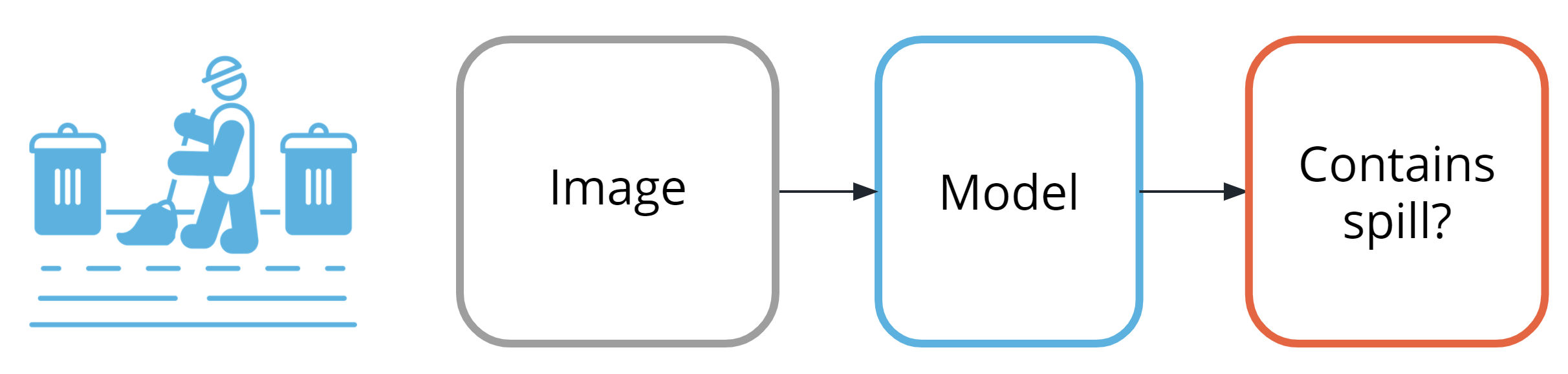
This task is a supervised classification task, as shown in the following image. As shown in the image above, your goal will be to predict if each image belongs to one of the following classes:
- Contains spill
- Does not contain spill
Traditionally, solving this problem would require hand-engineering features on top of the underlying pixels (for example, locations of prominent edges and corners in the image), and then training a model on these features.
Today, deep neural networks are the most common tool used for solving this kind of problem. Many deep neural network models are structured to learn the features on top of the underlying pixels so you don’t have to learn them. You’ll have a chance to take a deeper look at this in the next lesson, so we’ll keep things high-level for now.
CNN (convolutional neural network)
Neural networks are beyond the scope of this lesson, but you can think of them as a collection of very simple models connected together. These simple models are called neurons, and the connections between these models are trainable model parameters called weights.
Convolutional Neural Networks are a special type of neural network particularly good at processing images.
Step Four: Model Evaluation
As you saw in the last example, there are many different statistical metrics you can use to evaluate your model. As you gain more experience in machine learning, you will learn how to research which metrics can help you evaluate your model most effectively. Here’s a list of common metrics:
| Accuracy | False positive rate | Precision |
| Confusion matrix | False negative rate | Recall |
| F1 Score | Log Loss | ROC curve |
| Negative predictive value | Specificity |
In cases such as this, accuracy might not be the best evaluation mechanism.
Why not? You realize the model will see the ‘Does not contain spill‘ class almost all the time, so any model that just predicts “no spill” most of the time will seem pretty accurate.
What you really care about is an evaluation tool that rarely misses a real spill.
After doing some internet sleuthing, you realize this is a common problem and that Precision and Recall will be effective. You can think of precision as answering the question, “Of all predictions of a spill, how many were right?” and recall as answering the question, “Of all actual spills, how many did we detect?”
Manual evaluation plays an important role. You are unsure if your staged spills are sufficiently realistic compared to actual spills. To get a better sense how well your model performs with actual spills, you find additional examples from historical records. This allows you to confirm that your model is performing satisfactorily.
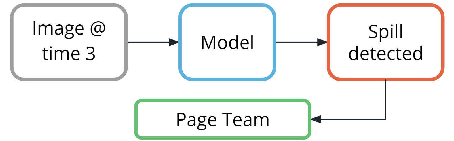
Step Five: Model Inference
The model can be deployed on a system that enables you to run machine learning workloads such as AWS Panorama.
Thankfully, most of the time, the results will be from the class ‘Does not contain spill.’
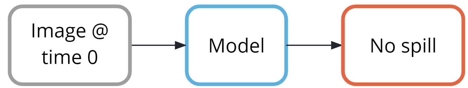
But, when the class ‘Contains spill‘ is detected, a simple paging system could alert the team to respond.
Terminology
- Convolutional neural networks(CNN) are a special type of neural network particularly good at processing images.
- Neural networks: a collection of very simple models connected together.
- These simple models are called neurons
- the connections between these models are trainable model parameters called weights.
Additional reading
As you continue your machine learning journey, you will start to recognize problems that are excellent candidates for machine learning.
The AWS Machine Learning Blog is a great resource for finding more examples of machine learning projects.
- In the Protecting people from hazardous areas through virtual boundaries with Computer Vision blog post, you can see a more detailed example of the deep learning process described in this lesson.
Quiz: Example Three
Now that you’ve seen a few examples, let’s double-check our understanding of the process. Match each step with an action you might take during that step.
| MACHINE LEARNING STEP | ACTION TAKEN AT THIS STEP |
|---|---|
| Step 1: Define the problem | Thinking of this problem as a classification task. |
| Step 2: Build the dataset | Flipping through photos to ensure the spill is clearly in shot. |
| Step 3: Train the model | Identifying a CNN as having a good chance of matching your data and task. |
| Step 4: Evaluate the model | Measuring model accuracy alone won’t give you confidence that the trained model is performing as intended. |
| Step 5: Use the model | Deploying the model to a system capable of processing images in the surveillance system. |
Final Quiz
Only a single metric can be used to evaluate a machine learning model.
True
False
Complete this phrase. There may be more than one correct answer.
A loss function…
is a model hyperparameter.
is a model parameter.
measures how close the model is towards its goal.
The model training algorithm iteratively updates a model’s parameters to minimize some loss function.
True
False
Supervised learning uses labeled data while training a model, and unsupervised learning uses unlabeled data while training a model.
True
False
Lesson Review
Congratulations on making it through the lesson. Let’s review what you learning
- In the first part of the lesson, we talked about what machine learning actually is, introduced you to some of the most common terms and ideas used in machine learning, and identified the common components involved in machine learning projects.
- We learned that machine learning involves using trained models to generate predictions and detect patterns from data. We looked behind the scenes to see what is really happening. We also broke down the different steps or tasks involved in machine learning.
- We looked at three machine learning examples to demonstrate how each works to solve real-world situations.
- A supervised learning task in which you used machine learning to predict housing prices for homes in your neighborhood, based on the lot size and the number of bedrooms.
- An unsupervised learning task in which you used machine learning to find interesting collections of books in a book dataset, based on the descriptive words in the book description text.
- Using a deep neural network to detect chemical spills in a lab from video and images.
Learning Objectives
If you watched all the videos, read through all the text and images, and completed all the quizzes, then you should’ve mastered the learning objectives for the lesson. You should recognize all of these by now. Please read through and check off each as you go through them.
Differentiate between supervised learning and unsupervised learning.
Identify problems that can be solved with machine learning.
Describe commonly used algorithms including linear regression, logistic regression, and k-means.
Describe how model training and testing works.
Evaluate the performance of a machine learning model using metrics.
Glossary
Bag of words: A technique used to extract features from the text. It counts how many times a word appears in a document (corpus), and then transforms that information into a dataset.
A categorical label has a discrete set of possible values, such as “is a cat” and “is not a cat.”
Clustering. Unsupervised learning task that helps to determine if there are any naturally occurring groupings in the data.
CNN: Convolutional Neural Networks (CNN) represent nested filters over grid-organized data. They are by far the most commonly used type of model when processing images.
A continuous (regression) label does not have a discrete set of possible values, which means possibly an unlimited number of possibilities.
Data vectorization: A process that converts non-numeric data into a numerical format so that it can be used by a machine learning model.
Discrete: A term taken from statistics referring to an outcome taking on only a finite number of values (such as days of the week).
FFNN: The most straightforward way of structuring a neural network, the Feed Forward Neural Network (FFNN) structures neurons in a series of layers, with each neuron in a layer containing weights to all neurons in the previous layer.
Hyperparameters are settings on the model which are not changed during training but can affect how quickly or how reliably the model trains, such as the number of clusters the model should identify.
Log loss is used to calculate how uncertain your model is about the predictions it is generating.
Hyperplane: A mathematical term for a surface that contains more than two planes.
Impute is a common term referring to different statistical tools which can be used to calculate missing values from your dataset.
label refers to data that already contains the solution.
loss function is used to codify the model’s distance from this goal (loss function is a model Hyperparameter).
Machine learning, or ML, is a modern software development technique that enables computers to solve problems by using examples of real-world data.
Model accuracy is the fraction of predictions a model gets right.
Discrete: A term taken from statistics referring to an outcome taking on only a finite number of values (such as days of the week).
Continuous: Floating-point values with an infinite range of possible values. The opposite of categorical or discrete values, which take on a limited number of possible values.
Model inference is when the trained model is used to generate predictions.
Model is an extremely generic program, made specific by the data used to train it.
Model parameters are settings or configurations the training algorithm can update to change how the model behaves.
Model training algorithms work through an interactive process where the current model iteration is analyzed to determine what changes can be made to get closer to the goal. Those changes are made and the iteration continues until the model is evaluated to meet the goals.
Neural networks: a collection of very simple models connected together. These simple models are called neurons. The connections between these models are trainable model parameters called weights.
Outliers are data points that are significantly different from others in the same sample.
Plane: A mathematical term for a flat surface (like a piece of paper) on which two points can be joined by a straight line.
Regression: A common task in supervised machine learning.
In reinforcement learning, the algorithm figures out which actions to take in a situation to maximize a reward (in the form of a number) on the way to reaching a specific goal.
RNN/LSTM: Recurrent Neural Networks (RNN) and the related Long Short-Term Memory (LSTM) model types are structured to effectively represent for loops in traditional computing, collecting state while iterating over some object. They can be used for processing sequences of data.
Silhouette coefficient: A score from -1 to 1 describing the clusters found during modeling. A score near zero indicates overlapping clusters, and scores less than zero indicate data points assigned to incorrect clusters. A score approaching 1 indicates successful identification of discrete non-overlapping clusters.
Stop words: A list of words removed by natural language processing tools when building your dataset. There is no single universal list of stop words used by all-natural language processing tools.
In supervised learning, every training sample from the dataset has a corresponding label or output value associated with it. As a result, the algorithm learns to predict labels or output values.
Test dataset: The data withheld from the model during training, which is used to test how well your model will generalize to new data.
Training dataset: The data on which the model will be trained. Most of your data will be here.
Transformer: A more modern replacement for RNN/LSTMs, the transformer architecture enables training over larger datasets involving sequences of data.
In unlabeled data, you don’t need to provide the model with any kind of label or solution while the model is being trained.
In unsupervised learning, there are no labels for the training data. A machine learning algorithm tries to learn the underlying patterns or distributions that govern the data.
Machine Learning with AWS
Machine Learning with AWS
Why AWS?
The AWS machine learning mission is to put machine learning in the hands of every developer.
- AWS offers the broadest and deepest set of artificial intelligence (AI) and machine learning (ML) services with unmatched flexibility.
- You can accelerate your adoption of machine learning with AWS SageMaker. Models that previously took months to build and required specialized expertise can now be built in weeks or even days.
- AWS offers the most comprehensive cloud offering optimized for machine learning.
- More machine learning happens at AWS than anywhere else.
AWS Machine Learning offerings
AWS AI services
By using AWS pre-trained AI services, you can apply ready-made intelligence to a wide range of applications such as personalized recommendations, modernizing your contact center, improving safety and security, and increasing customer engagement.
Industry-specific solutions
With no knowledge in machine learning needed, add intelligence to a wide range of applications in different industries including healthcare and manufacturing.
AWS Machine Learning services
With AWS, you can build, train, and deploy your models fast. Amazon SageMaker is a fully managed service that removes complexity from ML workflows so every developer and data scientist can deploy machine learning for a wide range of use cases.
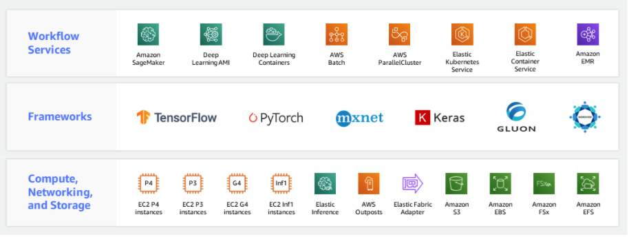
ML infrastructure and frameworks
AWS Workflow services make it easier for you to manage and scale your underlying ML infrastructure.
Getting started
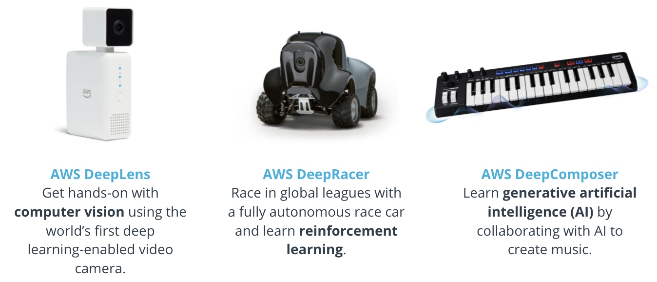
In addition to educational resources such as AWS Training and Certification, AWS has created a portfolio of educational devices to help put new machine learning techniques into the hands of developers in unique and fun ways, with AWS DeepLens, AWS DeepRacer, and AWS DeepComposer.
- AWS DeepLens: A deep learning–enabled video camera
- AWS DeepRacer: An autonomous race car designed to test reinforcement learning models by racing on a physical track
- AWS DeepComposer: A composing device powered by generative AI that creates a melody that transforms into a completely original song
- AWS ML Training and Certification: Curriculum used to train Amazon developers
Additional Reading
- To learn more about AWS AI Services, see Explore AWS AI services.
- To learn more about AWS ML Training and Certification offerings, see Training and Certification.
Lesson Overview
In this lesson, you’ll get an introduction to machine learning (ML) with AWS and AWS AI devices: AWS DeepLens, AWS DeepComposer, and AWS DeepRacer. Learn the basics of computer vision with AWS DeepLens, race around a track and get familiar with reinforcement learning with AWS DeepRacer, and discover the power of generative AI by creating music using AWS DeepComposer.

By the end of the lesson, you will be able to:
- Identify AWS machine learning offerings and understand how different services are used for different applications.
- Explain the fundamentals of computer vision and provide examples of popular tasks.
- Describe how reinforcement learning works in the context of AWS DeepRacer.
- Explain the fundamentals of generative AI and its applications, and describe three famous generative AI models in the context of music and AWS DeepComposer.
AWS Account Requirements
An AWS account is required
To complete the exercises in this course, you need an AWS Account ID.
To set up a new AWS Account ID, follow the directions in How do I create and activate a new Amazon Web Services account?
You are required to provide a payment method when you create the account. To learn about which services are available at no cost, see the AWS Free Tier documentation.
Will these exercises cost anything?
This lesson contains many demos and exercises. You do not need to purchase any AWS devices to complete the lesson. However, please carefully read the following list of AWS services you may need in order to follow the demos and complete the exercises.
Train your computer vision model with AWS DeepLens (optional)
- To train and deploy custom models to AWS DeepLens, you use Amazon SageMaker. Amazon SageMaker is a separate service and has its own service pricing and billing tier. It’s not required to train a model for this course. If you’re interested in training a custom model, please note that it incurs a cost. To learn more about SageMaker costs, see the Amazon SageMaker Pricing.
Train your reinforcement learning model with AWS DeepRacer
- To get started with AWS DeepRacer, you receive 10 free hours to train or evaluate models and 5GB of free storage during your first month. This is enough to train your first time-trial model, evaluate it, tune it, and then enter it into the AWS DeepRacer League. This offer is valid for 30 days after you have used the service for the first time.
- Beyond 10 hours of training and evaluation, you pay for training, evaluating, and storing your machine learning models. Charges are based on the amount of time you train and evaluate a new model and the size of the model stored. To learn more about AWS DeepRacer pricing, see the AWS DeepRacer Pricing
Generate music using AWS DeepComposer
- To get started, AWS DeepComposer provides a 12-month Free Tier for first-time users. With the Free Tier, you can perform up to 500 inference jobs translating to 500 pieces of music using the AWS DeepComposer Music studio. You can use one of these instances to complete the exercise at no cost. To learn more about AWS DeepComposer costs, see the AWS DeepComposer Pricing.
Build a custom generative AI model (GAN) using Amazon SageMaker (optional)
- Amazon SageMaker is a separate service and has its own service pricing and billing tier. To train the custom generative AI model, the instructor uses an instance type that is not covered in the Amazon SageMaker free tier. If you want to code along with the instructor and train your own custom model, you may incur a cost. Please note, that creating your own custom model is completely optional. You are not required to do this exercise to complete the course. To learn more about SageMaker costs, see the Amazon SageMaker Pricing.
Computer Vision and Its Applications
This section introduces you to common concepts in computer vision (CV), and explains how you can use AWS DeepLens to start learning with computer vision projects. By the end of this section, you will be able to explain how to create, train, deploy, and evaluate a trash-sorting project that uses AWS DeepLens.
Introduction to Computer Vision
Summary
Computer vision got its start in the 1960s in academia. Since its inception, it has been an interdisciplinary field. Machine learning practitioners use computers to understand and automate tasks associated with the visual word.
Modern-day applications of computer vision use neural networks. These networks can quickly be trained on millions of images and produce highly accurate predictions.
Since 2010, there has been exponential growth in the field of computer vision. You can start with simple tasks like image classification and objection detection and then scale all the way up to the nearly real-time video analysis required for self-driving cars to work at scale.
In the video, you have learned:
How computer vision got started
- Early applications of computer vision needed hand-annotated images to successfully train a model.
- These early applications had limited applications because of the human labor required to annotate images.
Three main components of neural networks
- Input Layer: This layer receives data during training and when inference is performed after the model has been trained.
- Hidden Layer: This layer finds important features in the input data that have predictive power based on the labels provided during training.
- Output Layer: This layer generates the output or prediction of your model.
Modern computer vision
- Modern-day applications of computer vision use neural networks call convolutional neural networks or CNNs.
- In these neural networks, the hidden layers are used to extract different information about images. We call this process feature extraction.
- These models can be trained much faster on millions of images and generate a better prediction than earlier models.
How this growth occurred
- Since 2010, we have seen a rapid decrease in the computational costs required to train the complex neural networks used in computer vision.
- Larger and larger pre-labeled datasets have become generally available. This has decreased the time required to collect the data needed to train many models.
Computer Vision Applications
Summary
Computer vision (CV) has many real-world applications. In this video, we cover examples of image classification, object detection, semantic segmentation, and activity recognition. Here’s a brief summary of what you learn about each topic in the video:
- Image classification is the most common application of computer vision in use today. Image classification can be used to answer questions like What’s in this image? This type of task has applications in text detection or optical character recognition (OCR) and content moderation.
- Object detection is closely related to image classification, but it allows users to gather more granular detail about an image. For example, rather than just knowing whether an object is present in an image, a user might want to know if there are multiple instances of the same object present in an image, or if objects from different classes appear in the same image.
- Semantic segmentation is another common application of computer vision that takes a pixel-by-pixel approach. Instead of just identifying whether an object is present or not, it tries to identify down the pixel level which part of the image is part of the object.
- Activity recognition is an application of computer vision that is based around videos rather than just images. Video has the added dimension of time and, therefore, models are able to detect changes that occur over time.
New Terms
- Input Layer: The first layer in a neural network. This layer receives all data that passes through the neural network.
- Hidden Layer: A layer that occurs between the output and input layers. Hidden layers are tailored to a specific task.
- Output Layer: The last layer in a neural network. This layer is where the predictions are generated based on the information captured in the hidden layers.
Additional Reading
- You can use the AWS DeepLens Recipes website to find different learning paths based on your level of expertise. For example, you can choose either a student or teacher path. Additionally, you can choose between beginner, intermediate, and advanced projects which have been created and vetted by the AWS DeepLens team.
- You can check out the AWS machine learning blog to learn about recent advancements in machine learning. Additionally, you can use the AWS DeepLens tag to see projects which have been created by the AWS DeepLens team.
- Ready to get started? Check out the Getting started guide in the AWS DeepLens Developer Guide.
Computer Vision with AWS DeepLens
AWS DeepLens
AWS DeepLens allows you to create and deploy end-to-end computer vision–based applications. The following video provides a brief introduction to how AWS DeepLens works and how it uses other AWS services.
Summary
AWS DeepLens is a deep learning–enabled camera that allows you to deploy trained models directly to the device. You can either use sample templates and recipes or train your own model.
AWS DeepLens is integrated with several AWS machine learning services and can perform local inference against deployed models provisioned from the AWS Cloud. It enables you to learn and explore the latest artificial intelligence (AI) tools and techniques for developing computer vision applications based on a deep learning model.
The AWS DeepLens device
The AWS DeepLens camera is powered by an Intel® Atom processor, which can process 100 billion floating-point operations per second (GFLOPS). This gives you all the computing power you need to perform inference on your device. The micro HDMI display port, audio out, and USB ports allow you to attach peripherals, so you can get creative with your computer vision applications.
You can use AWS DeepLens as soon as you register it.

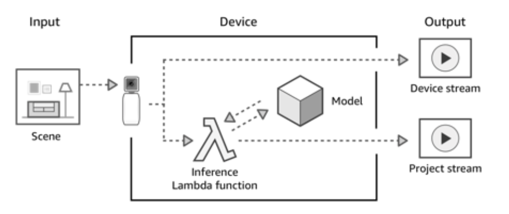
How AWS DeepLens works
AWS DeepLens is integrated with multiple AWS services. You use these services to create, train, and launch your AWS DeepLens project. You can think of an AWS DeepLens project as being divided into two different streams as the image shown above.
- First, you use the AWS console to create your project, store your data, and train your model.
- Then, you use your trained model on the AWS DeepLens device. On the device, the video stream from the camera is processed, inference is performed, and the output from inference is passed into two output streams:
- Device stream – The video stream passed through without processing.
- Project stream – The results of the model’s processing of the video frames.
Additional Reading
- To learn more about the specifics of the AWS DeepLens device, see the AWS DeepLens Hardware Specifications in the AWS DeepLens Developer Guide.
- You can buy an AWS DeepLens device on Amazon.com.
A Sample Project with AWS DeepLens
This section provides a hands-on demonstration of a project created as part of an AWS DeepLens sponsored hack-a-thon. In this project, we use an AWS DeepLens device to do an image classification–based task. We train a model to detect if a piece of trash is from three potential classes: landfill, compost, or recycling.
Important
- Storing data, training a model, and using AWS Lambda to deploy your model incur costs on your AWS account. For more information, see the AWS account requirements page.
- You are not required to follow this demo on the AWS console. However, we recommend you watch it and understand the flow of completing a computer vision project with AWS DeepLens.
Demo Part 1: Getting Setup and Running the Code
Summary: demo part 1
In this demo, you first saw how you can use Amazon S3 to store the image data needed for training your computer vision model. Then, you saw how to use Amazon SageMaker to train your model using a Jupyter Notebook
Demo Part 2: Deployment and Testing
Summary: demo part 2
Next, you used AWS Lambda to deploy your model onto an AWS DeepLens device. Finally, once your model has been deployed to your device, you can use AWS IoT Greengrass to view the inference output from your model actively running on your AWS DeepLens device.
Lab
More Projects on AWS DeepLens and Other AWS Services
- In this blog post on the AWS Machine Learning blog, you learn about how computer vision–based applications can be used to protect workers in workplaces with autonomous robots. The post demonstrates you how you can create a virtual boundary using a computer and AWS DeepLens.
- Using Amazon Rekognition and AWS DeepLens, you can create an application that uses OCR or optical character recognition to recognize a car’s license plate, and open a garage door.
- You can use Amazon Alexa and AWS DeepLens to create a Pictionary style game. First, you deploy a trained model to your AWS DeepLens which can recognize sketches drawn on a whiteboard and pair it with an Alexa skill that serves as the official scorekeeper.
Quiz: Computer Vision

To detect both the cat and the dog present in this image, what kind of computer vision model would you use?
Image classification
Object detection
Semantic segmentation
Activity recognition
Which computer vision–based task would you use to detect that the dog in the image is sleeping?
Image classification
Object detection
Semantic segmentation
Activity recognition
Which computer vision–based task would you use to detect the exact location of the cat and dog in the image?
Image classification
Object detection
Semantic segmentation
Activity recognition
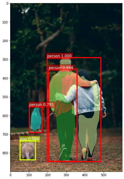
In the preceding image, which computer vision–based task would you use to identify where the people and the dog are?
Image classification
Object detection
Semantic segmentation
Activity recognition

In the preceding image, what kind of computer vision model would you use to count the number of cars?
Image classification
Object detection
Semantic segmentation
Activity recognition
Which of the following are computer vision tasks? Select all the answers that apply.
Object detection
Semantic segmentation
Generative adversarial networks
Natural language processing
Reinforcement learning
What type of computer vision task is the trash-sorting project?
Image classification
Object detection
Semantic segmentation
Activity recognition
Reinforcement Learning and Its Applications
This section introduces you to a type of machine learning (ML) called reinforcement learning (RL). You’ll hear about its real-world applications and learn basic concepts using AWS DeepRacer as an example. By the end of the section, you will be able to create, train, and evaluate a reinforcement learning model in the AWS DeepRacer console.
Introduction to Reinforcement Learning
Summary
In reinforcement learning (RL), an agent is trained to achieve a goal based on the feedback it receives as it interacts with an environment. It collects a number as a reward for each action it takes. Actions that help the agent achieve its goal are incentivized with higher numbers. Unhelpful actions result in a low reward or no reward.
With a learning objective of maximizing total cumulative reward, over time, the agent learns, through trial and error, to map gainful actions to situations. The better trained the agent, the more efficiently it chooses actions that accomplish its goal.
Reinforcement Learning Applications
Summary
Reinforcement learning is used in a variety of fields to solve real-world problems. It’s particularly useful for addressing sequential problems with long-term goals. Let’s take a look at some examples.
RL is great at playing games:
- Go (board game) was mastered by the AlphaGo Zero software.
- Atari classic video games are commonly used as a learning tool for creating and testing RL software.
- StarCraft II, the real-time strategy video game, was mastered by the AlphaStar software.
RL is used in video game level design:
- Video game level design determines how complex each stage of a game is and directly affects how boring, frustrating, or fun it is to play that game.
- Video game companies create an agent that plays the game over and over again to collect data that can be visualized on graphs.
- This visual data gives designers a quick way to assess how easy or difficult it is for a player to make progress, which enables them to find that “just right” balance between boredom and frustration faster.
RL is used in wind energy optimization:
- RL models can also be used to power robotics in physical devices.
- When multiple turbines work together in a wind farm, the turbines in the front, which receive the wind first, can cause poor wind conditions for the turbines behind them. This is called wake turbulence and it reduces the amount of energy that is captured and converted into electrical power.
- Wind energy organizations around the world use reinforcement learning to test solutions. Their models respond to changing wind conditions by changing the angle of the turbine blades. When the upstream turbines slow down it helps the downstream turbines capture more energy.
Other examples of real-world RL include:
- Industrial robotics
- Fraud detection
- Stock trading
- Autonomous driving
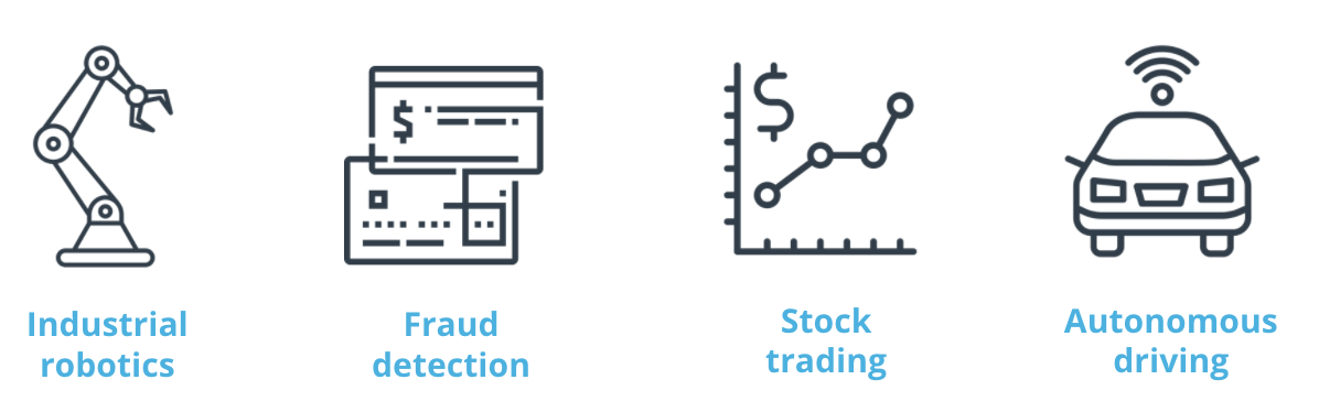
New Terms
- Agent: The piece of software you are training is called an agent. It makes decisions in an environment to reach a goal.
- Environment: The environment is the surrounding area with which the agent interacts.
- Reward: Feedback is given to an agent for each action it takes in a given state. This feedback is a numerical reward.
- Action: For every state, an agent needs to take an action toward achieving its goal.
Reinforcement Learning with AWS DeepRacer
Reinforcement Learning Concepts
In this section, we’ll learn some basic reinforcement learning terms and concepts using AWS DeepRacer as an example.
Summary
This section introduces six basic reinforcement learning terms and provides an example for each in the context of AWS DeepRacer.
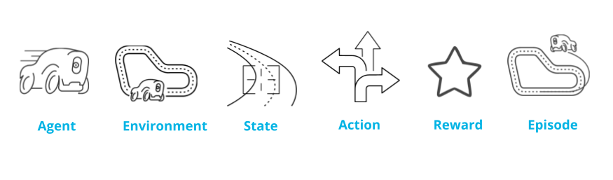
Agent
- The piece of software you are training is called an agent.
- It makes decisions in an environment to reach a goal.
- In AWS DeepRacer, the agent is the AWS DeepRacer car and its goal is to finish * laps around the track as fast as it can - while, in some cases, avoiding obstacles.
Environment
- The environment is the surrounding area within which our agent interacts.
- For AWS DeepRacer, this is a track in our simulator or in real life.
State
- The state is defined by the current position within the environment that is visible, or known, to an agent.
- In AWS DeepRacer’s case, each state is an image captured by its camera.
- The car’s initial state is the starting line of the track and its terminal state is when the car finishes a lap, bumps into an obstacle, or drives off the track.
Action
- For every state, an agent needs to take an action toward achieving its goal.
- An AWS DeepRacer car approaching a turn can choose to accelerate or brake and turn left, right, or go straight.
Reward
- Feedback is given to an agent for each action it takes in a given state.
- This feedback is a numerical reward.
- A reward function is an incentive plan that assigns scores as rewards to different zones on the track.
Episode
- An episode represents a period of trial and error when an agent makes decisions and gets feedback from its environment.
- For AWS DeepRacer, an episode begins at the initial state, when the car leaves the starting position, and ends at the terminal state, when it finishes a lap, bumps into an obstacle, or drives off the track.
In a reinforcement learning model, an agent learns in an interactive real-time environment by trial and error using feedback from its own actions. Feedback is given in the form of rewards.
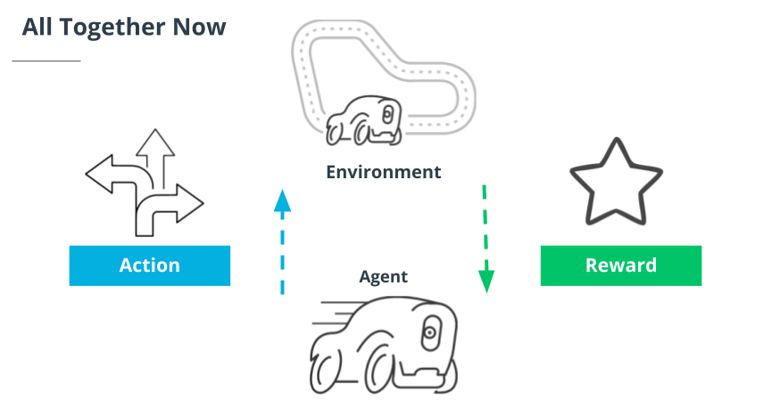
In a reinforcement learning model, an agent learns in an interactive real-time environment by trial and error using feedback from its own actions. Feedback is given in the form of rewards.
Putting Your Spin on AWS DeepRacer: The Practitioner’s Role in RL
Summary
AWS DeepRacer may be autonomous, but you still have an important role to play in the success of your model. In this section, we introduce the training algorithm, action space, hyperparameters, and reward function and discuss how your ideas make a difference.
- An algorithm is a set of instructions that tells a computer what to do. ML is special because it enables computers to learn without being explicitly programmed to do so.
- The training algorithm defines your model’s learning objective, which is to maximize total cumulative reward. Different algorithms have different strategies for going about this.
- A soft actor critic (SAC) embraces exploration and is data-efficient, but can lack stability.
- A proximal policy optimization (PPO) is stable but data-hungry.
- An action space is the set of all valid actions, or choices, available to an agent as it interacts with an environment.
- Discrete action space represents all of an agent’s possible actions for each state in a finite set of steering angle and throttle value combinations.
- Continuous action space allows the agent to select an action from a range of values that you define for each state.
- Hyperparameters are variables that control the performance of your agent during training. There is a variety of different categories with which to experiment. Change the values to increase or decrease the influence of different parts of your model.
- For example, the learning rate is a hyperparameter that controls how many new experiences are counted in learning at each step. A higher learning rate results in faster training but may reduce the model’s quality.
- The reward function‘s purpose is to encourage the agent to reach its goal. Figuring out how to reward which actions is one of your most important jobs.
Putting Reinforcement Learning into Action with AWS DeepRacer
Summary
This video put the concepts we’ve learned into action by imagining the reward function as a grid mapped over the race track in AWS DeepRacer’s training environment, and visualizing it as metrics plotted on a graph. It also introduced the trade-off between exploration and exploitation, an important challenge unique to this type of machine learning.
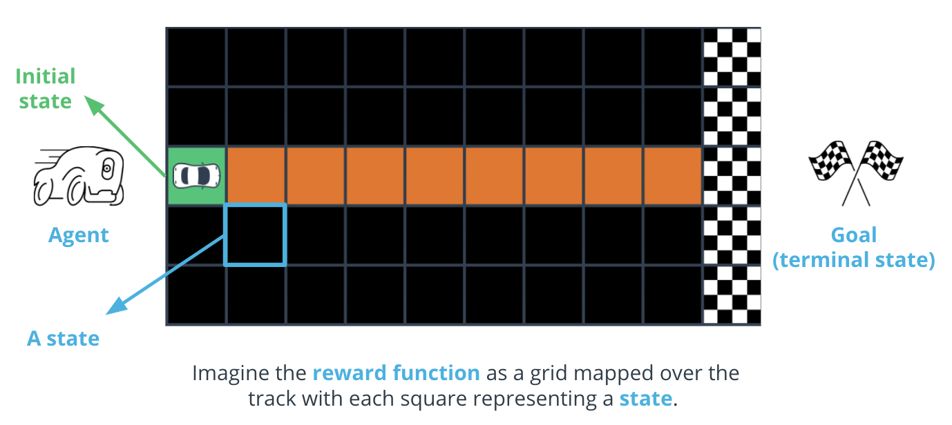
Each square is a state. The green square is the starting position, or initial state, and the finish line is the goal, or terminal state.
Key points to remember about reward functions:
- Each state on the grid is assigned a score by your reward function. You incentivize behavior that supports your car’s goal of completing fast laps by giving the highest numbers to the parts of the track on which you want it to drive.
- The reward function is the actual code you’ll write to help your agent determine if the action it just took was good or bad, and how good or bad it was.
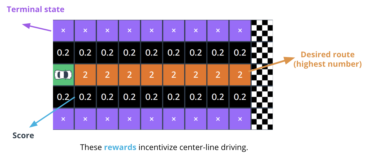
The squares containing [x] are the track edges and defined as terminal states, which tell your car it has gone off track.
Key points to remember about exploration versus exploitation:
- When a car first starts out, it explores by wandering in random directions. However, the more training an agent gets, the more it learns about an environment. This experience helps it become more confident about the actions it chooses.
- Exploitation means the car begins to exploit or use information from previous experiences to help it reach its goal. Different training algorithms utilize exploration and exploitation differently.
Key points to remember about the reward graph:
- While training your car in the AWS DeepRacer console, your training metrics are displayed on a reward graph.
- Plotting the total reward from each episode allows you to see how the model performs over time. The more reward your car gets, the better your model performs.
Key points to remember about AWS DeepRacer:
- AWS DeepRacer is a combination of a physical car and a virtual simulator in the AWS Console, the AWS DeepRacer League, and community races.
- An AWS DeepRacer device is not required to start learning: you can start now in the AWS console. The 3D simulator in the AWS console is where training and evaluation take place.
New Terms
- Exploration versus exploitation: An agent should exploit known information from previous experiences to achieve higher cumulative rewards, but it also needs to explore to gain new experiences that can be used in choosing the best actions in the future.
Additional Reading
- If you are interested in more tips, workshops, classes, and other resources for improving your model, you’ll find a wealth of resources on the AWS DeepRacer Pit Stop page.
- For detailed step-by-step instructions and troubleshooting support, see the AWS DeepRacer Developer Documentation.
- If you’re interested in reading more posts on a range of DeepRacer topics as well as staying up to date on the newest releases, check out the AWS Discussion Forums.
- If you’re interested in connecting with a thriving global community of reinforcement learning racing enthusiasts, join the AWS DeepRacer Slack community.
If you’re interested in tinkering with DeepRacer’s open-source device software and collaborating with robotics innovators, check out our AWS DeepRacer GitHub Organization.
Demo: Reinforcement Learning with AWS DeepRacer
To get you started with AWS DeepRacer, you receive 10 free hours to train or evaluate models and 5GB of free storage during your first month. This offer is valid for 30 days after you have used the service for the first time. Beyond 10 hours of training and evaluation, you pay for training, evaluating, and storing your machine learning models. Please read the AWS account requirements page for more information.
Demo Part 1: Create your car
Click here to go to the AWS DeepRacer console.
Summary
This demonstration introduces you to the AWS DeepRacer console and walks you through how to use it to build your first reinforcement learning model. You’ll use your knowledge of basic reinforcement learning concepts and terminology to make choices about your model. In addition, you’ll learn about the following features of the AWS DeepRacer service:
- Pro and Open Leagues
- Digital rewards
- Racer profile
- Garage
- Sensor configuration
- Race types
- Time trial
- Object avoidance
- Head-to-head
Demo Part 2: Train your car
This demonstration walks you through the training process in the AWS DeepRacer console. You’ve learned about:
- The reward graph
- The training video
Demo Part 3: Testing your car
Summary
This demonstration walks the evaluation process in the AWS DeepRacer console.
Once you’ve created a successful model, you’ll learn how to enter it into a race for the chance to win awards, prizes, and the opportunity to compete in the worldwide AWS DeepRacer Championship.
Lab
Quiz: Reinforcement Learning
In which type of machine learning are models trained using labeled data?
Reinforcement learning
Supervised learning
Unsupervised learning
In reinforcement learning, what is an “agent”?
A tool for designing an incentive plan which specifies which actions will be rewarded.
The piece of software you are training that makes decisions in an environment to reach a goal.
A popular supervised learning technique that is used to predict continuous values in house prices
TRUE or FALSE: In reinforcement learning, “Exploration” is using experience to decide.
FALSE
TRUE
How does a balance of “Exploration” and “Exploitation” help a reinforcement learning model?
The more an agent learns about its environment, the more confident it becomes about the action it chooses.
If an agent doesn’t explore enough, it often sticks to information its already learned even if this knowledge doesn’t help the agent achieve its goal.
The agent can use information from previous experiences to help it make future decisions that enable it to reach its goal.
An agent should not explore an environment because random actions just lead to low reward.
The reward function gives an agent all the information it needs to reach its goal.
| TERM | DEFINITION |
|---|---|
| State | The current position within the environment that is visible, or known, to an agent |
| Action | For every state, an agent needs to do this toward achieving its goal. |
| Episode | Represents a period of trial and error when an agent makes decision and gets feedback from its environment. |
| Reward | Feedback given to an agent for each action it takes in a given state. |
| Environment | The surrounding area our agent interacts with. |
AWS DeepRacer Reinforcement Learning Exercise
Exercise Solution: AWS DeepRacer
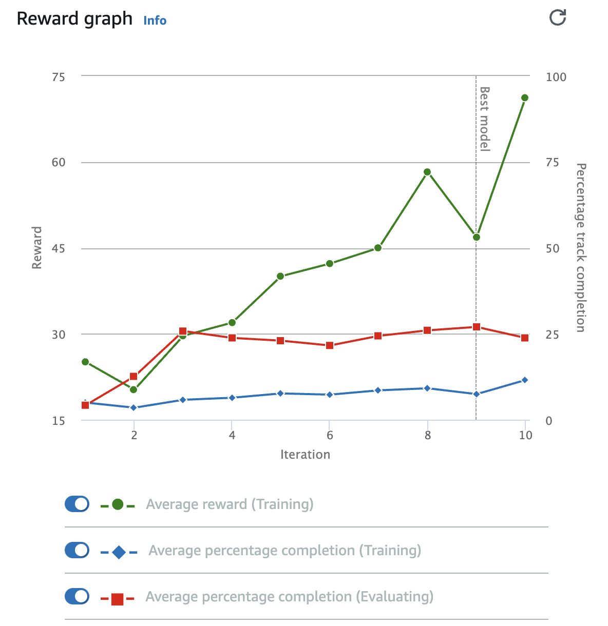
Exercise Solution
To get a sense of how well your training is going, watch the reward graph. Here is a list of its parts and what they do:
- Average reward
- This graph represents the average reward the agent earns during a training iteration. The average is calculated by averaging the reward earned across all episodes in the training iteration. An episode begins at the starting line and ends when the agent completes one loop around the track or at the place the vehicle left the track or collided with an object. Toggle the switch to hide this data.
- Average percentage completion (training)
- The training graph represents the average percentage of the track completed by the agent in all training episodes in the current training. It shows the performance of the vehicle while experience is being gathered.
Average percentage completion (evaluation)
- While the model is being updated, the performance of the existing model is evaluated. The evaluation graph line is the average percentage of the track completed by the agent in all episodes run during the evaluation period.
- Best model line
- This line allows you to see which of your model iterations had the highest average progress during the evaluation. The checkpoint for this iteration will be stored. A checkpoint is a snapshot of a model that is captured after each training (policy-updating) iteration.
- Reward primary y-axis
- This shows the reward earned during a training iteration. To read the exact value of a reward, hover your mouse over the data point on the graph.
- Percentage track completion secondary y-axis
- This shows you the percentage of the track the agent completed during a training iteration.
Iteration x-axis
- This shows the number of iterations completed during your training job.
Reward Graph Interpretation
The following four examples give you a sense of how to interpret the success of your model based on the reward graph. Learning to read these graphs is as much of an art as it is a science and takes time, but reviewing the following four examples will give you a start.
Needs more training
In the following example, we see there have only been 600 iterations, and the graphs are still going up. We see the evaluation completion percentage has just reached 100%, which is a good sign but isn’t fully consistent yet, and the training completion graph still has a ways to go. This reward function and model are showing promise, but need more training time.
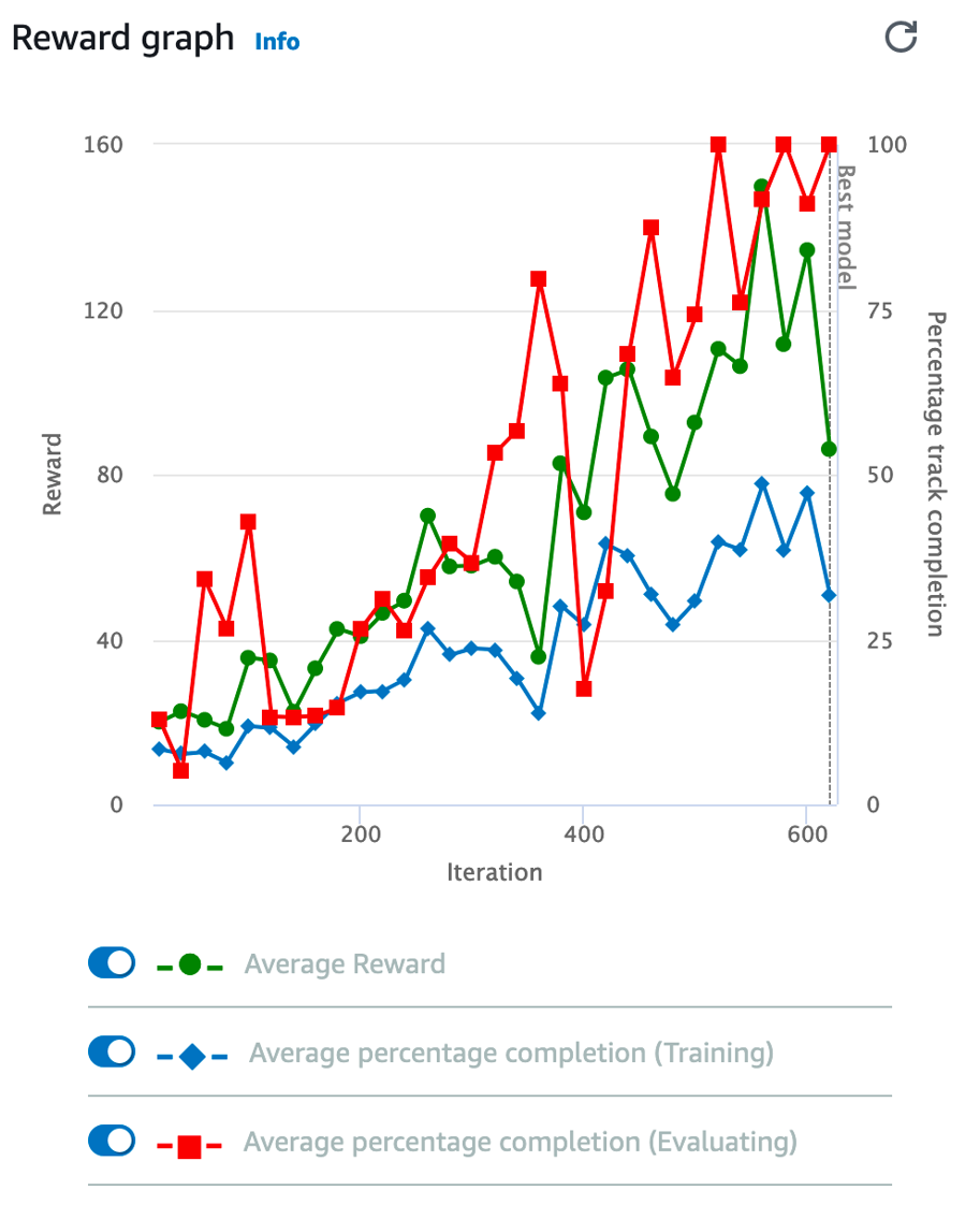
No improvement
In the next example, we can see that the percentage of track completions haven’t gone above around 15 percent and it’s been training for quite some time—probably around 6000 iterations or so. This is not a good sign! Consider throwing this model and reward function away and trying a different strategy.
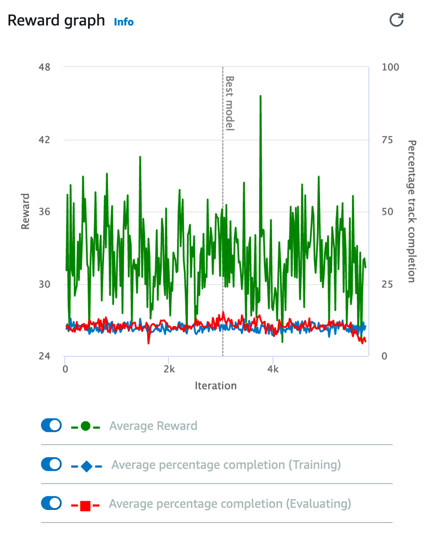
A well-trained model
In the following example graph, we see the evaluation percentage completion reached 100% a while ago, and the training percentage reached 100% roughly 100 or so iterations ago. At this point, the model is well trained. Training it further might lead to the model becoming overfit to this track.
Avoid overfitting
Overfitting or overtraining is a really important concept in machine learning. With AWS DeepRacer, this can become an issue when a model is trained on a specific track for too long. A good model should be able to make decisions based on the features of the road, such as the sidelines and centerlines, and be able to drive on just about any track.
An overtrained model, on the other hand, learns to navigate using landmarks specific to an individual track. For example, the agent turns a certain direction when it sees uniquely shaped grass in the background or a specific angle the corner of the wall makes. The resulting model will run beautifully on that specific track, but perform badly on a different virtual track, or even on the same track in a physical environment due to slight variations in angles, textures, and lighting.
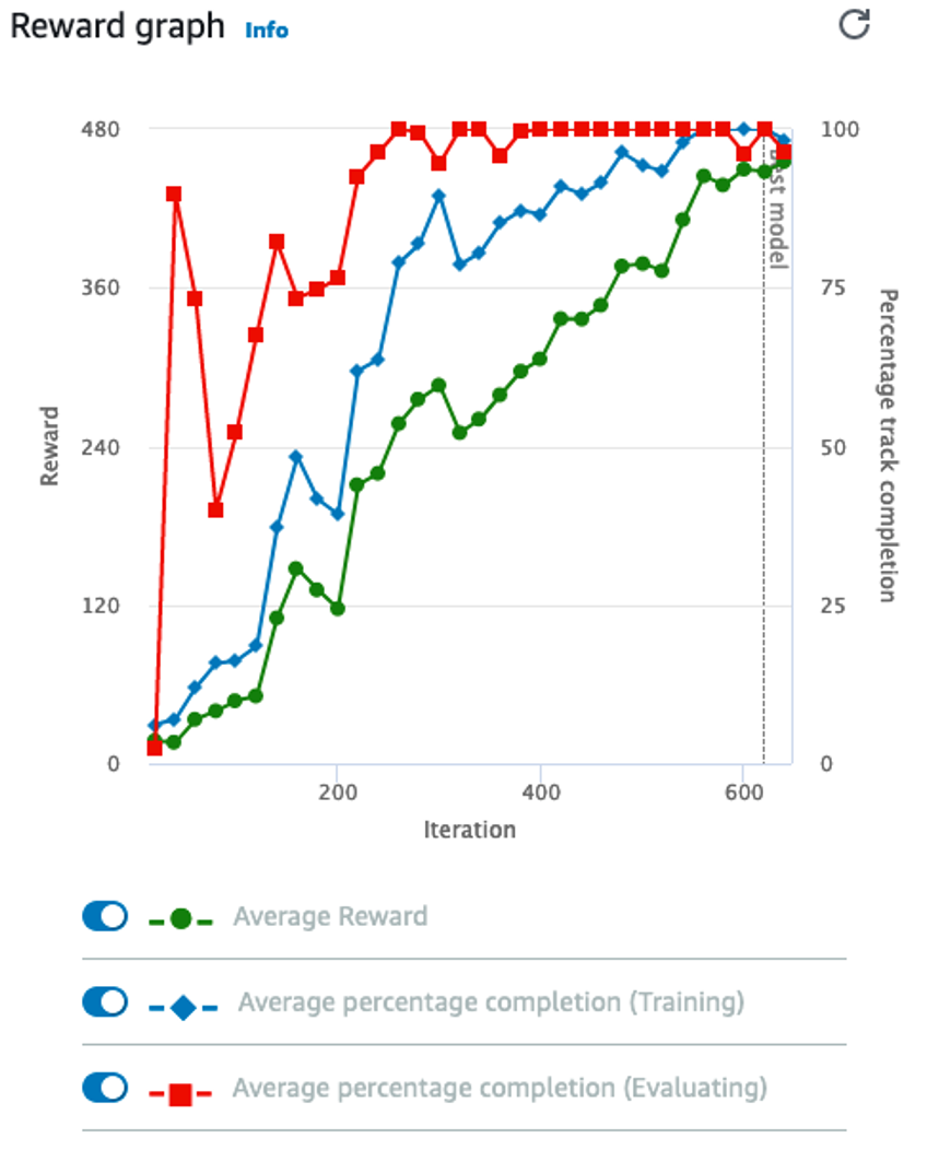
Adjust hyperparameters
The AWS DeepRacer console’s default hyperparameters are quite effective, but occasionally you may consider adjusting the training hyperparameters. The hyperparameters are variables that essentially act as settings for the training algorithm that control the performance of your agent during training. We learned, for example, that the learning rate controls how many new experiences are counted in learning at each step.
In this reward graph example, the training completion graph and the reward graph are swinging high and low. This might suggest an inability to converge, which may be helped by adjusting the learning rate. Imagine if the current weight for a given node is .03, and the optimal weight should be .035, but your learning rate was set to .01. The next training iteration would then swing past optimal to .04, and the following iteration would swing under it to .03 again. If you suspect this, you can reduce the learning rate to .001. A lower learning rate makes learning take longer but can help increase the quality of your model.
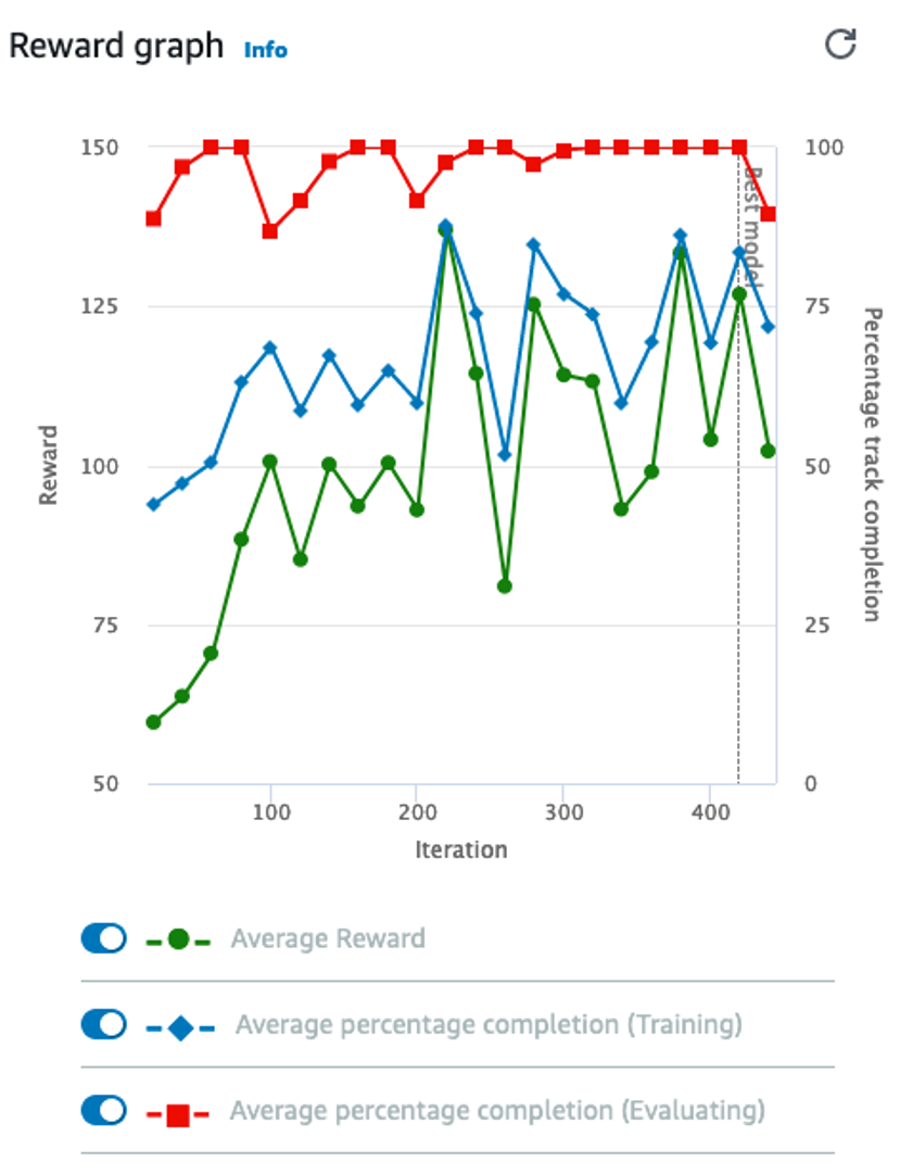
Good Job and Good Luck!
Remember: training experience helps both model and reinforcement learning practitioners become a better team. Enter your model in the monthly AWS DeepRacer League races for chances to win prizes and glory while improving your machine learning development skills!
Introduction to Generative AI
Generative AI and Its Applications
Generative AI is one of the biggest recent advancements in artificial intelligence because of its ability to create new things.
Until recently, the majority of machine learning applications were powered by discriminative models. A discriminative model aims to answer the question, “If I’m looking at some data, how can I best classify this data or predict a value?” For example, we could use discriminative models to detect if a camera was pointed at a cat.
As we train this model over a collection of images (some of which contain cats and others which do not), we expect the model to find patterns in images which help make this prediction.
A generative model aims to answer the question,”Have I seen data like this before?” In our image classification example, we might still use a generative model by framing the problem in terms of whether an image with the label “cat” is more similar to data you’ve seen before than an image with the label “no cat.”
However, generative models can be used to support a second use case. The patterns learned in generative models can be used to create brand new examples of data which look similar to the data it seen before.
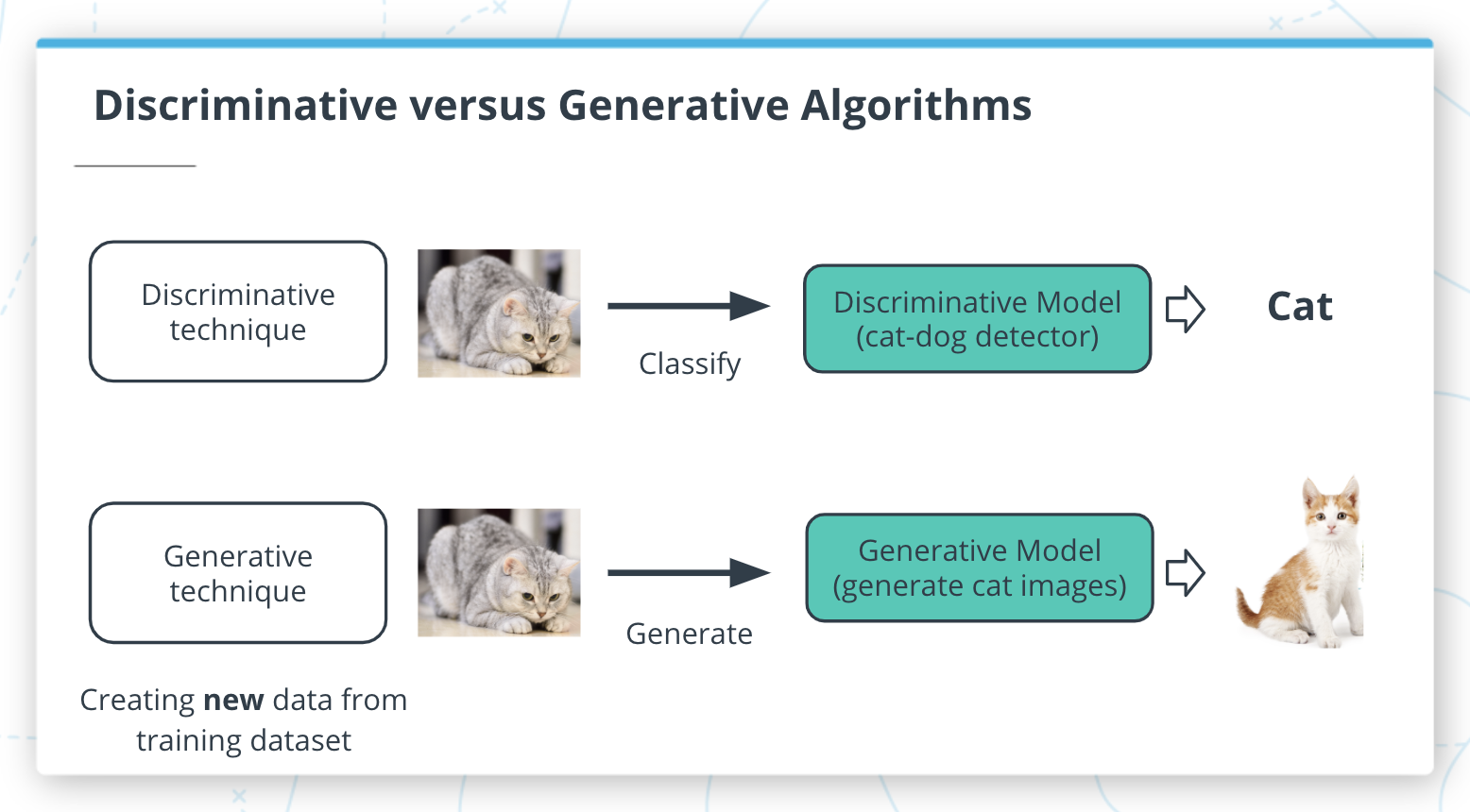
Generative AI Models
In this lesson, you will learn how to create three popular types of generative models: generative adversarial networks (GANs), general autoregressive models, and transformer-based models. Each of these is accessible through AWS DeepComposer to give you hands-on experience with using these techniques to generate new examples of music.
Autoregressive models
Autoregressive convolutional neural networks (AR-CNNs) are used to study systems that evolve over time and assume that the likelihood of some data depends only on what has happened in the past. It’s a useful way of looking at many systems, from weather prediction to stock prediction.
Generative adversarial networks (GANs)
Generative adversarial networks (GANs), are a machine learning model format that involves pitting two networks against each other to generate new content. The training algorithm swaps back and forth between training a generator network (responsible for producing new data) and a discriminator network (responsible for measuring how closely the generator network’s data represents the training dataset).
Transformer-based models
Transformer-based models are most often used to study data with some sequential structure (such as the sequence of words in a sentence). Transformer-based methods are now a common modern tool for modeling natural language.
We won’t cover this approach in this course but you can learn more about transformers and how AWS DeepComposer uses transformers in AWS DeepComposer learning capsules.
Generative AI with AWS DeepComposer
What is AWS DeepComposer?
AWS DeepComposer gives you a creative and easy way to get started with machine learning (ML), specifically generative AI. It consists of a USB keyboard that connects to your computer to input melody and the AWS DeepComposer console, which includes AWS DeepComposer Music studio to generate music, learning capsules to dive deep into generative AI models, and AWS DeepComposer Chartbusters challenges to showcase your ML skills.

Summary
AWS DeepComposer keyboard
You don’t need an AWS DeepComposer keyboard to finish this course. You can import your own MIDI file, use one of the provided sample melodies, or use the virtual keyboard in the AWS DeepComposer Music studio.
AWS DeepComposer music studio
To generate, create, and edit compositions with AWS DeepComposer, you use the AWS DeepComposer Music studio. To get started, you need an input track and a trained model.
For the input track, you can use a sample track, record a custom track, or import a track.
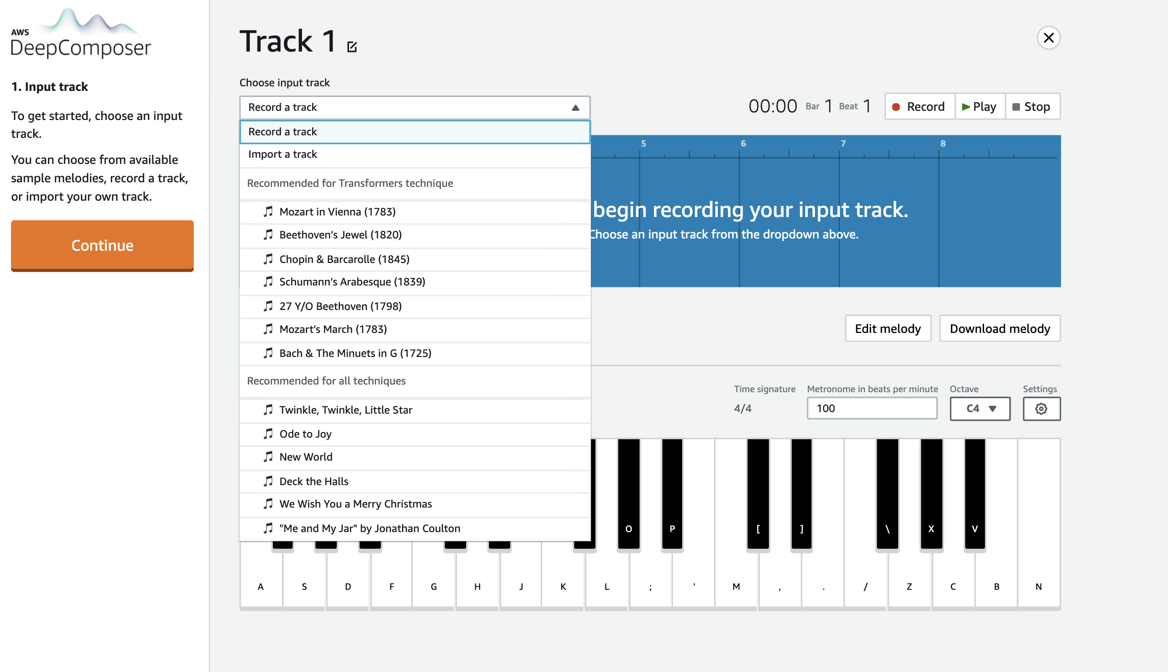
For the ML technique, you can use either a sample model or a custom model.
Each AWS DeepComposer Music studio experience supports three different generative AI techniques: generative adversarial networks (GANs), autoregressive convolutional neural network (AR-CNNs), and transformers.
- Use the GAN technique to create accompaniment tracks.
- Use the AR-CNN technique to modify notes in your input track.
- Use the transformers technique to extend your input track by up to 30 seconds.
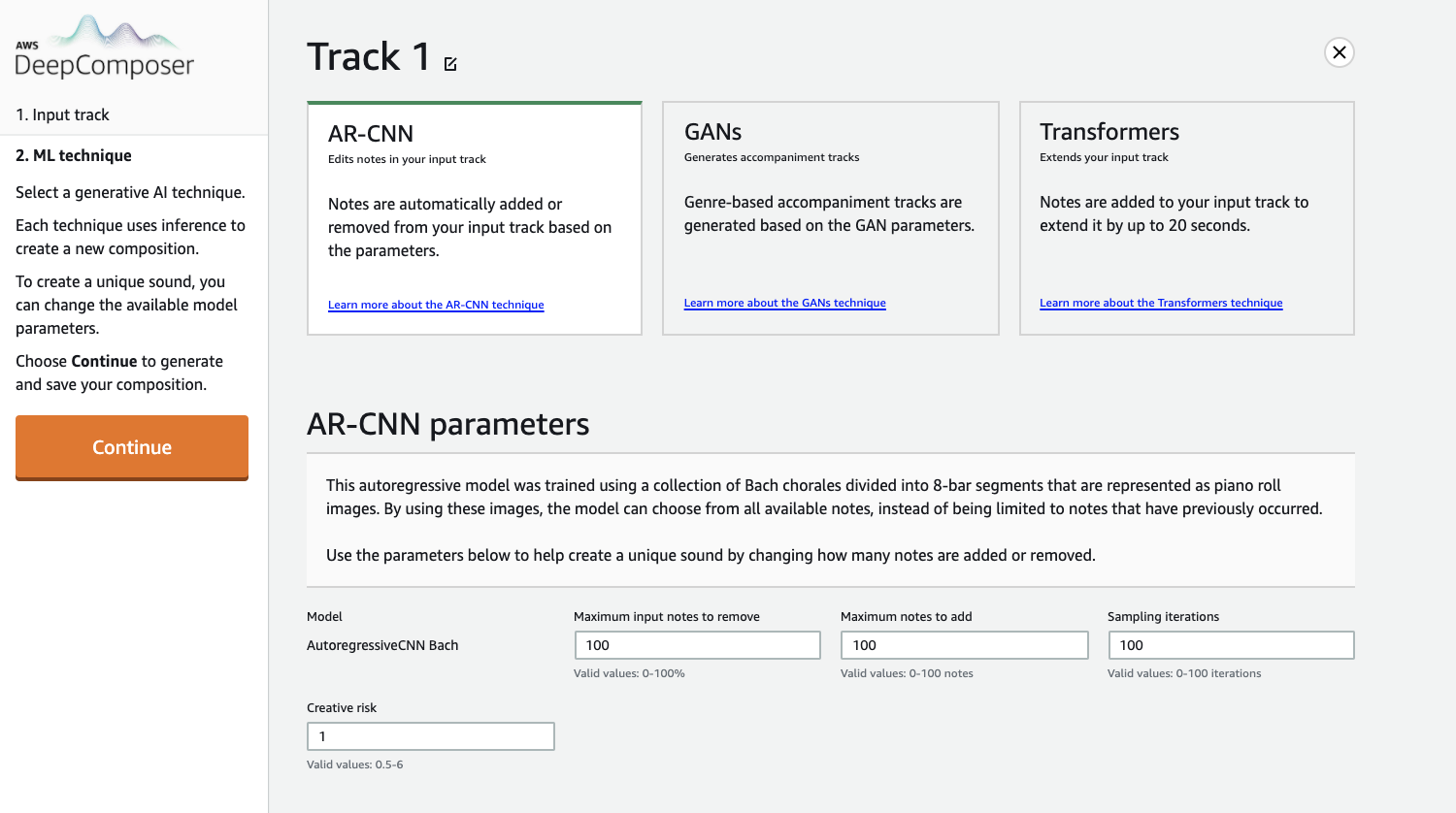
Demo: AWS DeepComposer
Summary
In this demo, you went through the AWS DeepComposer console where you can learn about deep learning, input your music, and train deep learning models to create new music.
AWS DeepComposer learning capsules
To learn the details behind generative AI and ML techniques used in AWS DeepComposer you can use easy-to-consume, bite-sized learning capsules in the AWS DeepComposer console.

AWS DeepComposer Chartbusters challenges
Chartbusters is a global challenge where you can use AWS DeepComposer to create original compositions and compete in monthly challenges to showcase your machine learning and generative AI skills.
You don’t need to participate in this challenge to finish this course, but the course teaches everything you need to win in both challenges we launched this season. Regardless of your background in music or ML, you can find a competition just right for you.
You can choose between two different challenges this season:
- In the Basic challenge, “Melody-Go-Round“, you can use any machine learning technique in the AWS DeepComposer Music studio to create new compositions.
- In the Advanced challenge, “Melody Harvest“, you train a custom generative AI model using Amazon SageMaker.
GANs with AWS DeepComposer
Summary
We’ll begin our journey of popular generative models in AWS DeepComposer with generative adversarial networks or GANs. Within an AWS DeepComposer GAN, models are used to solve a creative task: adding accompaniments that match the style of an input track you provide. Listen to the input melody and the output composition created by the AWS DeepComposer GAN model:
What are GANs?
A GAN is a type of generative machine learning model which pits two neural networks against each other to generate new content: a generator and a discriminator.
- A generator is a neural network that learns to create new data resembling the source data on which it was trained.
- A discriminator is another neural network trained to differentiate between real and synthetic data.
The generator and the discriminator are trained in alternating cycles. The generator learns to produce more and more realistic data while the discriminator iteratively gets better at learning to differentiate real data from the newly created data.
Collaboration between an orchestra and its conductor
A simple metaphor of an orchestra and its conductor can be used to understand a GAN. The orchestra trains, practices, and tries to generate polished music, and then the conductor works with them, as both judge and coach. The conductor judges the quality of the output and at the same time provides feedback to achieve a specific style. The more they work together, the better the orchestra can perform.
The GAN models that AWS DeepComposer uses work in a similar fashion. There are two competing networks working together to learn how to generate musical compositions in distinctive styles.
A GAN’s generator produces new music as the orchestra does. And the discriminator judges whether the music generator creates is realistic and provides feedback on how to make its data more realistic, just as a conductor provides feedback to make an orchestra sound better.

Training Methodology
Let’s dig one level deeper by looking at how GANs are trained and used within AWS DeepComposer. During training, the generator and discriminator work in a tight loop as depicted in the following image.
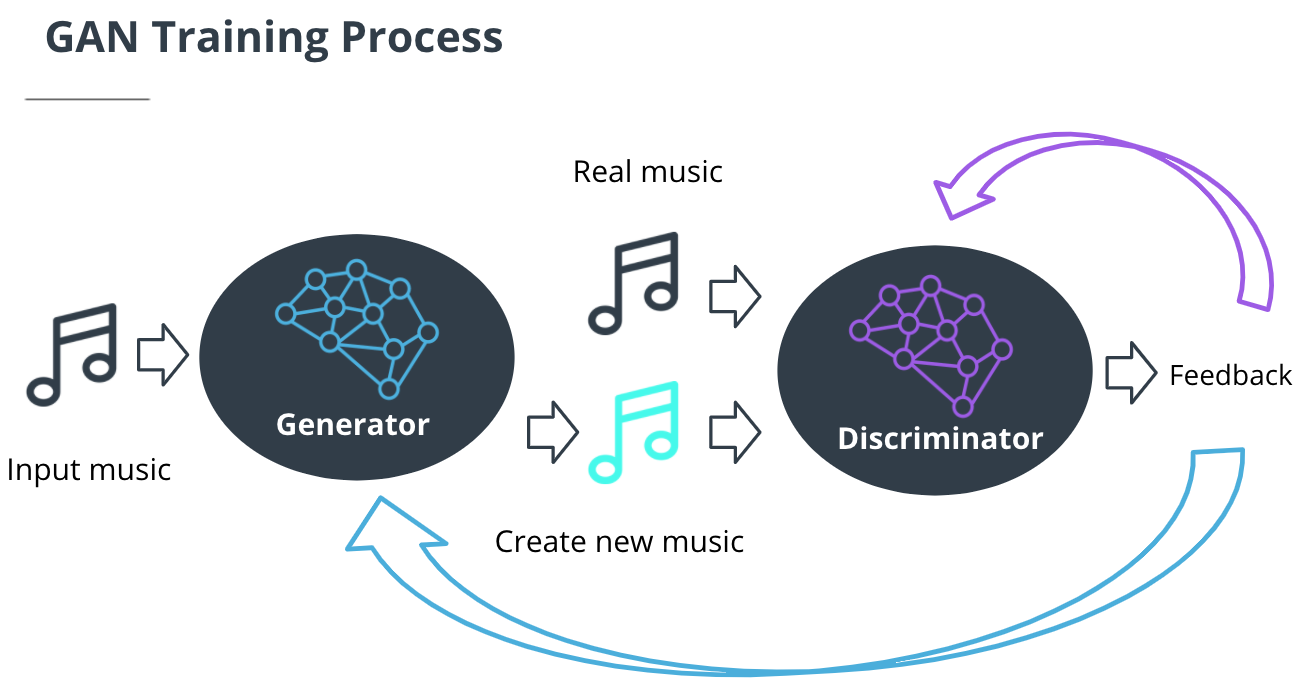
Note: While this figure shows the generator taking input on the left, GANs in general can also generate new data without any input.
Generator
- The generator takes in a batch of single-track piano rolls (melody) as the input and generates a batch of multi-track piano rolls as the output by adding accompaniments to each of the input music tracks.
- The discriminator then takes these generated music tracks and predicts how far they deviate from the real data present in the training dataset. This deviation is called the generator loss. This feedback from the discriminator is used by the generator to incrementally get better at creating realistic output.
Discriminator
- As the generator gets better at creating music accompaniments, it begins fooling the discriminator. So, the discriminator needs to be retrained as well. The discriminator measures the discriminator loss to evaluate how well it is differentiating between real and fake data.
Beginning with the discriminator on the first iteration, we alternate training these two networks until we reach some stop condition; for example, the algorithm has seen the entire dataset a certain number of times or the generator and discriminator loss reach some plateau (as shown in the following image).
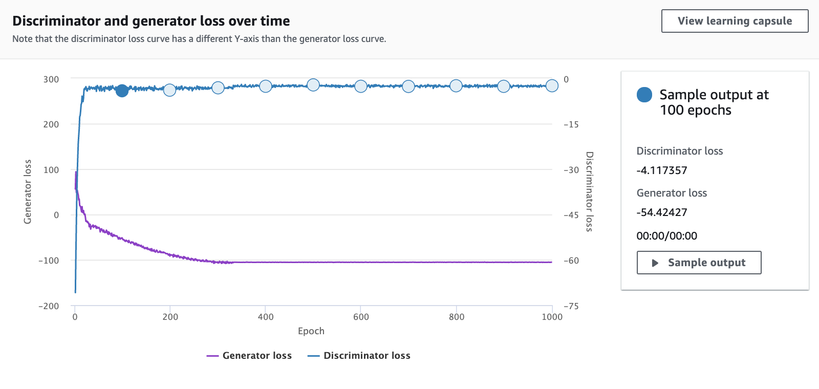
New Terms
- Generator: A neural network that learns to create new data resembling the source data on which it was trained.
- Discriminator: A neural network trained to differentiate between real and synthetic data.
- Generator loss: Measures how far the output data deviates from the real data present in the training dataset.
- Discriminator loss: Evaluates how well the discriminator differentiates between real and fake data.
Support Materials
AR-CNN with AWS DeepComposer
Summary
Our next popular generative model is the autoregressive convolutional neural network (AR-CNN). Autoregressive convolutional neural networks make iterative changes over time to create new data.
To better understand how the AR-CNN model works, let’s first discuss how music is represented so it is machine-readable.
Image-based representation
Nearly all machine learning algorithms operate on data as numbers or sequences of numbers. In AWS DeepComposer, the input tracks are represented as a piano roll. In each two-dimensional piano roll, time is on the horizontal axis and pitch is on the vertical axis. You might notice this representation looks similar to an image.
The AR-CNN model uses a piano roll image to represent the audio files from the dataset. You can see an example in the following image where on top is a musical score and below is a piano roll image of that same score.
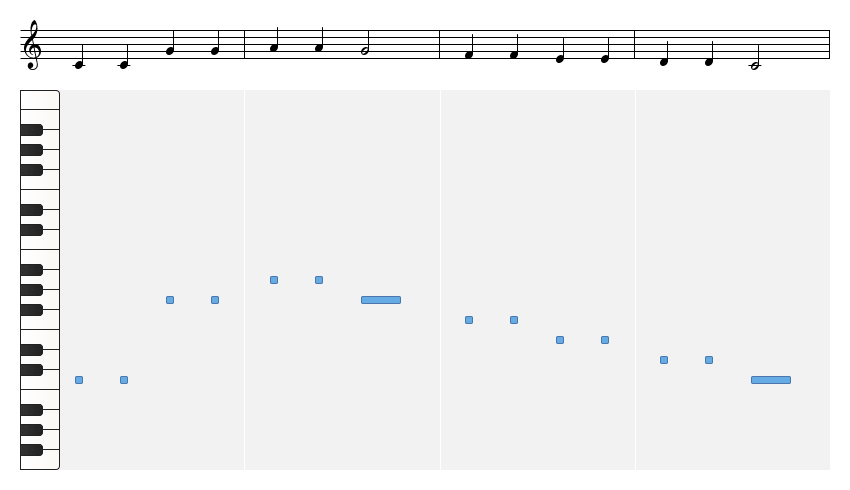
How the AR-CNN Model Works
When a note is either added or removed from your input track during inference, we call it an edit event. To train the AR-CNN model to predict when notes need to be added or removed from your input track (edit event), the model iteratively updates the input track to sounds more like the training dataset. During training, the model is also challenged to detect differences between an original piano roll and a newly modified piano roll.
New Terms
- Piano roll: A two-dimensional piano roll matrix that represents input tracks. Time is on the horizontal axis and pitch is on the vertical axis.
- Edit event: When a note is either added or removed from your input track during inference.
Quiz: Generative AI
Which is the following statements is false in the context of AR-CNNs?
2D images can be used to represent music.
AR-CNN generates output music iteratively over time.
“Edit event” refers to a note added to the input track during inference.
Autoregressive model can be used to study weather forecasting.
Please identify which of the following statements are true about a generative adversarial network (GAN). There may be more than one correct answer.
The generator and discriminator both use source data only.
The generator learns leans to produce more realistic data and the discriminator learns to differentiate real data from the newly created data.
The discriminator learns from both real Bach music and realistic Bach music.
The generator is responsible for both creating new music and providing feedback.
Which model is responsible for each of these roles in generative AI?
| Roles | Name |
|---|---|
| Evaluating the output quality | Discriminator |
| Creating new output | Generator |
| Providing feedback | Discriminator |
True or false: Loss functions help us determine when to stop training a model.
True
False
Demo: Create Music with AWS DeepComposer
Below you find a video demonstrating how you can use AWS DeepComposer to experiment with GANs and AR-CNN models.
Important
- To get you started, AWS DeepComposer provides a 12-month Free Tier for first-time users. With the Free Tier, you can perform up to 500 inference jobs, translating to 500 pieces of music, using the AWS DeepComposer Music studio. You can use one of these instances to complete the exercise at no cost. For more information, please read the AWS account requirements page.
Demo Part 1:
Demo Part 2:
Summary
In the demo, you have learned how to create music using AWS Deepcomposer.
You will need a music track to get started. There are several ways to do it. You can record your own using the AWS keyboard device or the virtual keyboard provided in the console. Or you can input a MIDI file or choose a provided music track.
Once the music track is inputted, choose “Continue” to create a model. The models you can choose are AR-CNN, GAN, and transformers. Each of them has a slightly different function. After choosing a model, you can then adjust the parameters used to train the model.
Once you are done with model creation, you can select “Continue” to listen and improve your output melody. To edit the melody, you can either drag or extend notes directly on the piano roll or adjust the model parameters and train it again. Keep tuning your melody until you are happy with it then click “Continue” to finish the composition.
If you want to enhance your music further with another generative model, you can do it too. Simply choose a model under the “Next step” section and create a new model to enhance your music.
Congratulations on creating your first piece of music using AWS DeepComposer! Now you can download the melody or submit it to a competition. Hope you enjoy the journey of creating music with AWS DeepComposer.
Exercise: Generate music with AWS DeepComposer
Build a Custom GAN Model (Optional): Part 1
Build a Custom GAN Model (Optional): Part 1
Build a Custom GAN Model
Build a Custom GAN Model (Optional): Part 2
Build a Custom GAN Model (Optional): Part 2
Build a Custom GAN Model
Lesson Review

In this lesson, we learned many advanced machine learning techniques. Specifically, we learned:
- Computer vision and its application
- How to train a computer vision project with AWS DeepLens
- Reinforcement learning and its application
- How to train a reinforcement learning model with AWS DeepRacer
- Generative AI
- How to train a GAN and AR-CNN model with AWS DeepComposer
Now, you should be able to:
- Identify AWS machine learning offerings and how different services are used for different applications
- Explain the fundamentals of computer vision and a couple of popular tasks
- Describe how reinforcement learning works in the context of AWS DeepRacer
- Explain the fundamentals of Generative AI, its applications, and three famous generative AI model in the context of music and AWS DeepComposer
Glossary
- Action: For every state, an agent needs to take an action toward achieving its goal.
- Agent: The piece of software you are training is called an agent. It makes decisions in an environment to reach a goal.
- Discriminator: A neural network trained to differentiate between real and synthetic data.
- Discriminator loss: Evaluates how well the discriminator differentiates between real and fake data.
- Edit event: When a note is either added or removed from your input track during inference.
- Environment: The environment is the surrounding area within which the agent interacts.
- Exploration versus exploitation: An agent should exploit known information from previous experiences to achieve higher cumulative rewards, but it also needs to explore to gain new experiences that can be used in choosing the best actions in the future.
- Generator: A neural network that learns to create new data resembling the source data on which it was trained.
- Generator loss: Measures how far the output data deviates from the real data present in the training dataset.
- Hidden layer: A layer that occurs between the output and input layers. Hidden layers are tailored to a specific task.
- Input layer: The first layer in a neural network. This layer receives all data that passes through the neural network.
- Output layer: The last layer in a neural network. This layer is where the predictions are generated based on the information captured in the hidden layers.
- Piano roll: A two-dimensional piano roll matrix that represents input tracks. Time is on the horizontal axis and pitch is on the vertical axis.
- Reward: Feedback is given to an agent for each action it takes in a given state. This feedback is a numerical reward.
Resources
Neural Network
Software Engineering Practices, Part I
Introduction
In this lesson, you’ll learn about the following software engineering practices and how they apply in data science.
- Writing clean and modular code
- Writing efficient code
- Code refactoring
- Adding meaningful documentation
- Using version control
In the lesson following this one (part 2), you’ll also learn about the following software engineering practices:
- Testing
- Logging
- Code reviews
Clean and Modular Code
- Production code: Software running on production servers to handle live users and data of the intended audience. Note that this is different from production-quality code, which describes code that meets expectations for production in reliability, efficiency, and other aspects. Ideally, all code in production meets these expectations, but this is not always the case.
- Clean code: Code that is readable, simple, and concise. Clean production-quality code is crucial for collaboration and maintainability in software development.
- Modular code: Code that is logically broken up into functions and modules. Modular production-quality code that makes your code more organized, efficient, and reusable.
- Module: A file. Modules allow code to be reused by encapsulating them into files that can be imported into other files.
Which of the following describes code that is clean? Select all the answers that apply.
Repetitive
Simple
Readable
Vague
Concise
Making your code modular makes it easier to do which of the following things? There may be more than one correct answer.
Reuse your code
Write less code
Read your code
Collaborate your code
Refactoring Code
Refactoring Code
- Refactoring: Restructuring your code to improve its internal structure without changing its external functionality. This gives you a chance to clean and modularize your program after you’ve got it working.
- Since it isn’t easy to write your best code while you’re still trying to just get it working, allocating time to do this is essential to producing high-quality code. Despite the initial time and effort required, this really pays off by speeding up your development time in the long run.
- You become a much stronger programmer when you’re constantly looking to improve your code. The more you refactor, the easier it will be to structure and write good code the first time.
Writing Clean Code
Writing clean code: Meaningful names
Use meaningful names
- Be descriptive and imply type: For booleans, you can prefix with
is_orhas_to make it clear it is a condition. You can also use parts of speech to imply types, like using verbs for functions and nouns for variables. - Be consistent but clearly differentiate:
age_listandageis easier to differentiate thanagesandage. - Avoid abbreviations and single letters: You can determine when to make these exceptions based on the audience for your code. If you work with other data scientists, certain variables may be common knowledge. While if you work with full stack engineers, it might be necessary to provide more descriptive names in these cases as well. (Exceptions include counters and common math variables.)
- Long names aren’t the same as descriptive names: You should be descriptive, but only with relevant information. For example, good function names describe what they do well without including details about implementation or highly specific uses.
Try testing how effective your names are by asking a fellow programmer to guess the purpose of a function or variable based on its name, without looking at your code. Coming up with meaningful names often requires effort to get right.
Writing clean code: Nice whitespace
Use whitespace properly.
- Organize your code with consistent indentation: the standard is to use four spaces for each indent. You can make this a default in your text editor.
- Separate sections with blank lines to keep your code well organized and readable.
- Try to limit your lines to around 79 characters, which is the guideline given in the PEP 8 style guide. In many good text editors, there is a setting to display a subtle line that indicates where the 79 character limit is.
For more guidelines, check out the code layout section of PEP 8 in the following notes.
References
Quiz: Clean Code
Quiz: Categorizing tasks
Imagine you are writing a program that executes a number of tasks and categorizes each task based on its execution time. Below is a small snippet of this program. Which of the following naming changes could make this code cleaner? There may be more than one correct answer.
1 | t = end_time - start # compute execution time |
None
Rename the variable start to start_time to make it consistent with end_time
Rename the variable t to execution_time to make it more descriptive.
Rename the function category to categorize_task to math the part of speech.
Rename the variable c to category to make it more descriptive.
Quiz: Buying stocks
Imagine you analyzed several stocks and calculated the ideal price, or limit price, at which you’d want to buy each stock. You write a program to iterate through your stocks and buy it if the current price is below or equal to the limit price you computed. Otherwise, you put it on a watchlist. Below are three ways of writing this code. Which of the following is the most clean?
1 | # Choice A |
Choice A
Choice B
Choice C
Writing Modular Code
Writing Modular Code
Follow the tips below to write modular code.
Tip: DRY (Don’t Repeat Yourself)
Don’t repeat yourself! Modularization allows you to reuse parts of your code. Generalize and consolidate repeated code in functions or loops.
Tip: Abstract out logic to improve readability
Abstracting out code into a function not only makes it less repetitive, but also improves readability with descriptive function names. Although your code can become more readable when you abstract out logic into functions, it is possible to over-engineer this and have way too many modules, so use your judgement.
Tip: Minimize the number of entities (functions, classes, modules, etc.)
There are trade-offs to having function calls instead of inline logic. If you have broken up your code into an unnecessary amount of functions and modules, you’ll have to jump around everywhere if you want to view the implementation details for something that may be too small to be worth it. Creating more modules doesn’t necessarily result in effective modularization.
Tip: Functions should do one thing
Each function you write should be focused on doing one thing. If a function is doing multiple things, it becomes more difficult to generalize and reuse. Generally, if there’s an “and” in your function name, consider refactoring.
Tip: Arbitrary variable names can be more effective in certain functions
Arbitrary variable names in general functions can actually make the code more readable.
Tip: Try to use fewer than three arguments per function
Try to use no more than three arguments when possible. This is not a hard rule and there are times when it is more appropriate to use many parameters. But in many cases, it’s more effective to use fewer arguments. Remember we are modularizing to simplify our code and make it more efficient. If your function has a lot of parameters, you may want to rethink how you are splitting this up.
Exercise: Refactoring - Wine quality
In this exercise, you’ll refactor code that analyzes a wine quality dataset taken from the UCI Machine Learning Repository. Each row contains data on a wine sample, including several physicochemical properties gathered from tests, as well as a quality rating evaluated by wine experts.
Download the notebook file refactor_wine_quality.ipynb and the dataset winequality-red.csv. Open the notebook file using the Jupyter Notebook. Follow the instructions in the notebook to complete the exercise.
Supporting Materials
Solution: Refactoring – Wine quality
The following code shows the solution code. You can download the solution notebook file that contains the solution code.
1 | import pandas as pd |
My solution.
1 | import pandas as pd |
Supporting Materials
Efficient Code
Efficient Code
Knowing how to write code that runs efficiently is another essential skill in software development. Optimizing code to be more efficient can mean making it:
- Execute faster
- Take up less space in memory/storage
The project on which you’re working determines which of these is more important to optimize for your company or product. When you’re performing lots of different transformations on large
Optimizing - Common Books
Resources:
Exercise: Optimizing – Common books
We provide the code your coworker wrote to find the common book IDs in books_published_last_two_years.txt and all_coding_books.txt to obtain a list of recent coding books. Can you optimize it?
Download the notebook file optimizing_code_common_books.ipynb and the text files. Open the notebook file using the Jupyter Notebook. Follow the instructions in the notebook to complete the exercise.
You can also take a look at the example notebook optimizing_code_common_books_example.ipynb to help you finish the exercise.
Supporting Materials
- All Coding Books
- Books Published Last Two Years
- Optimizing Code Common Books
- Optimizing Code Common Books Example
Solution: Optimizing - Common books
The following code shows the solution code. You can download the solution notebook file that contains the solution code.
1 | import time |
Supporting Materials
Exercise: Optimizing - Holiday Gifts
In the last example, you learned that using vectorized operations and more efficient data structures can optimize your code. Let’s use these tips for one more exercise.
Your online gift store has one million users that each listed a gift on a wishlist. You have the prices for each of these gifts stored in gift_costs.txt. For the holidays, you’re going to give each customer their wishlist gift for free if the cost is under $25. Now, you want to calculate the total cost of all gifts under $25 to see how much you’d spend on free gifts.
Download the notebook file optimizing_code_holiday_gifts.ipynb and the gift_costs.txt file. Open the notebook file using the Jupyter Notebook. Follow the instructions in the notebook to complete the exercise.
Supporting Materials
Solution: Optimizing – Holiday gifts
The following code shows the solution code. You can download the solution notebook file that contains the solution code.
1 | import time |
My Solution
1 | # Refactoring Soltuion 1 |
Supporting Materials
Documentation
Documentation
- Documentation: Additional text or illustrated information that comes with or is embedded in the code of software.
- Documentation is helpful for clarifying complex parts of code, making your code easier to navigate, and quickly conveying how and why different components of your program are used.
- Several types of documentation can be added at different levels of your program:
- Inline comments - line level
- Docstrings - module and function level
- Project documentation - project level
Inline Comments
Inline Comments
- Inline comments are text following hash symbols throughout your code. They are used to explain parts of your code, and really help future contributors understand your work.
- Comments often document the major steps of complex code. Readers may not have to understand the code to follow what it does if the comments explain it. However, others would argue that this is using comments to justify bad code, and that if code requires comments to follow, it is a sign refactoring is needed.
- Comments are valuable for explaining where code cannot. For example, the history behind why a certain method was implemented a specific way. Sometimes an unconventional or seemingly arbitrary approach may be applied because of some obscure external variable causing side effects. These things are difficult to explain with code.
Docstrings
Docstrings
Docstring, or documentation strings, are valuable pieces of documentation that explain the functionality of any function or module in your code. Ideally, each of your functions should always have a docstring.
Docstrings are surrounded by triple quotes. The first line of the docstring is a brief explanation of the function’s purpose.
One-line docstring
1 | def population_density(population, land_area): |
If you think that the function is complicated enough to warrant a longer description, you can add a more thorough paragraph after the one-line summary.
Multi-line docstring
1 | def population_density(population, land_area): |
The next element of a docstring is an explanation of the function’s arguments. Here, you list the arguments, state their purpose, and state what types the arguments should be. Finally, it is common to provide some description of the output of the function. Every piece of the docstring is optional; however, doc strings are a part of good coding practice.
Resources
Project Documentation
Project documentation is essential for getting others to understand why and how your code is relevant to them, whether they are potentials users of your project or developers who may contribute to your code. A great first step in project documentation is your README file. It will often be the first interaction most users will have with your project.
Whether it’s an application or a package, your project should absolutely come with a README file. At a minimum, this should explain what it does, list its dependencies, and provide sufficiently detailed instructions on how to use it. Make it as simple as possible for others to understand the purpose of your project and quickly get something working.
Translating all your ideas and thoughts formally on paper can be a little difficult, but you’ll get better over time, and doing so makes a significant difference in helping others realize the value of your project. Writing this documentation can also help you improve the design of your code, as you’re forced to think through your design decisions more thoroughly. It also helps future contributors to follow your original intentions.
There is a full Udacity course on this topic.
Here are a few READMEs from some popular projects:
Quiz: Documentation
Which of the following statements about in-line comments are true? There may be more than one correct answer.
Comments are useful for clarifying complex code.
You never have too many comments.
Comments are only for unreadable parts of code.
Readable code is preferable over having comments to make your code readable.
Which of the following statements about docstrings are true?
Multiline docstrings are better than single line docstrings.
Docstrings explain the purpose of a function or module.
Docstrings and comments are interchangeable.
You can add whatever details you want in a docstring.
Not including a docstring will cause an error.
Version Control in Data Science
Version Control In Data Science
If you need a refresher on using Git for version control, check out the course linked in the extracurriculars. If you’re ready, let’s see how Git is used in real data science scenarios!
Scenario #1
Scenario #1
Let’s walk through the Git commands that go along with each step in the scenario you just observed in the video.
Step 1: You have a local version of this repository on your laptop, and to get the latest stable version, you pull from the develop branch.
1 | git checkout develop |
1 | git pull |
Step 2: When you start working on this demographic feature, you create a new branch called demographic, and start working on your code in this branch.
1 | git checkout -b demographic |
1 | git commit -m 'added gender recommendations' |
Step 3: However, in the middle of your work, you need to work on another feature. So you commit your changes on this demographic branch, and switch back to the develop branch.
1 | git commit -m 'refactored demographic gender and location recommendations ' |
1 | git checkout develop |
Step 4: From this stable develop branch, you create another branch for a new feature called friend_groups.
1 | git checkout -b friend_groups |
Step 5: After you finish your work on the friend_groups branch, you commit your changes, switch back to the development branch, merge it back to the develop branch, and push this to the remote repository’s develop branch.
1 | git commit -m 'finalized friend_groups recommendations ' |
1 | git checkout develop |
1 | git merge --no-ff friends_groups |
1 | git push origin develop |
Step 6: Now, you can switch back to the demographic branch to continue your progress on that feature.
1 | git checkout demographic |
Scenario #2
Scenario #2
Let’s walk through the Git commands that go along with each step in the scenario you just observed in the video.
Step 1: You check your commit history, seeing messages about the changes you made and how well the code performed.
1 | git log |
Step 2: The model at this commit seemed to score the highest, so you decide to take a look.
1 | git checkout bc90f2cbc9dc4e802b46e7a153aa106dc9a88560 |
After inspecting your code, you realize what modifications made it perform well, and use those for your model.
Step 3: Now, you’re confident merging your changes back into the development branch and pushing the updated recommendation engine.
1 | git checkout develop |
1 | git merge --no-ff friend_groups |
1 | git push origin develop |
Scenario #3
Scenario #3
Let’s walk through the Git commands that go along with each step in the scenario you just observed in the video.
Step 1: Andrew commits his changes to the documentation branch, switches to the development branch, and pulls down the latest changes from the cloud on this development branch, including the change I merged previously for the friends group feature.
1 | git commit -m "standardized all docstrings in process.py" |
1 | git checkout develop |
1 | git pull |
Step 2: Andrew merges his documentation branch into the develop branch on his local repository, and then pushes his changes up to update the develop branch on the remote repository.
1 | git merge --no-ff documentation |
1 | git push origin develop |
Step 3: After the team reviews your work and Andrew’s work, they merge the updates from the development branch into the master branch. Then, they push the changes to the master branch on the remote repository. These changes are now in production.
1 | git merge --no-ff develop |
1 | git push origin master |
Resources
Read this great article on a successful Git branching strategy.
Note on merge conflicts
For the most part, Git makes merging changes between branches really simple. However, there are some cases where Git can become confused about how to combine two changes, and asks you for help. This is called a merge conflict.
Mostly commonly, this happens when two branches modify the same file.
For example, in this situation, let’s say you deleted a line that Andrew modified on his branch. Git wouldn’t know whether to delete the line or modify it. You need to tell Git which change to take, and some tools even allow you to edit the change manually. If it isn’t straightforward, you may have to consult with the developer of the other branch to handle a merge conflict.
To learn more about merge conflicts and methods to handle them, see About merge conflicts.
Model versioning
In the previous example, you may have noticed that each commit was documented with a score for that model. This is one simple way to help you keep track of model versions. Version control in data science can be tricky, because there are many pieces involved that can be hard to track, such as large amounts of data, model versions, seeds, and hyperparameters.
The following resources offer useful methods and tools for managing model versions and large amounts of data. These are here for you to explore, but are not necessary to know now as you start your journey as a data scientist. On the job, you’ll always be learning new skills, and many of them will be specific to the processes set in your company.
Conclusion
Software Engineering Practices, part 2
Introduction
Welcome To Software Engineering Practices, Part 2
In part 2 of software engineering practices, you’ll learn about the following practices of software engineering and how they apply in data science.
- Testing
- Logging
- Code reviews
Testing
Testing
Testing your code is essential before deployment. It helps you catch errors and faulty conclusions before they make any major impact. Today, employers are looking for data scientists with the skills to properly prepare their code for an industry setting, which includes testing their code.
Testing and Data Science
Testing And Data Science
- Problems that could occur in data science aren’t always easily detectable; you might have values being encoded incorrectly, features being used inappropriately, or unexpected data breaking assumptions.
- To catch these errors, you have to check for the quality and accuracy of your analysis in addition to the quality of your code. Proper testing is necessary to avoid unexpected surprises and have confidence in your results.
- Test-driven development (TDD): A development process in which you write tests for tasks before you even write the code to implement those tasks.
- Unit test: A type of test that covers a “unit” of code—usually a single function—independently from the rest of the program.
Resources
- Four Ways Data Science Goes Wrong and How Test-Driven Data Analysis Can Help: Blog Post
- Ned Batchelder: Getting Started Testing: Slide Deck and Presentation Video
Unit Tests
Unit tests
We want to test our functions in a way that is repeatable and automated. Ideally, we’d run a test program that runs all our unit tests and cleanly lets us know which ones failed and which ones succeeded. Fortunately, there are great tools available in Python that we can use to create effective unit tests!
Unit test advantages and disadvantages
The advantage of unit tests is that they are isolated from the rest of your program, and thus, no dependencies are involved. They don’t require access to databases, APIs, or other external sources of information. However, passing unit tests isn’t always enough to prove that our program is working successfully. To show that all the parts of our program work with each other properly, communicating and transferring data between them correctly, we use integration tests. In this lesson, we’ll focus on unit tests; however, when you start building larger programs, you will want to use integration tests as well.
To learn more about integration testing and how integration tests relate to unit tests, see Integration Testing. That article contains other very useful links as well.
Unit Testing Tools
Unit Testing Tools
To install pytest, run pip install -U pytest in your terminal. You can see more information on getting started here.
- Create a test file starting with
test_. - Define unit test functions that start with
test_inside the test file. - Enter
pytestinto your terminal in the directory of your test file and it detects these tests for you.
test_ is the default; if you wish to change this, you can learn how in this pytest configuration.
In the test output, periods represent successful unit tests and Fs represent failed unit tests. Since all you see is which test functions failed, it’s wise to have only one assert statement per test. Otherwise, you won’t know exactly how many tests failed or which tests failed.
Your test won’t be stopped by failed assert statements, but it will stop if you have syntax errors.
Exercise: Unit tests
Download README.md, compute_launch.py, and test_compute_launch.py.
Follow the instructions in README.md to complete the exercise.
Supporting Materials
Test-driven development and data science
Test-driven development and data science
- Test-driven development: Writing tests before you write the code that’s being tested. Your test fails at first, and you know you’ve finished implementing a task when the test passes.
- Tests can check for different scenarios and edge cases before you even start to write your function. When start implementing your function, you can run the test to get immediate feedback on whether it works or not as you tweak your function.
- When refactoring or adding to your code, tests help you rest assured that the rest of your code didn’t break while you were making those changes. Tests also helps ensure that your function behavior is repeatable, regardless of external parameters such as hardware and time.
Test-driven development for data science is relatively new and is experiencing a lot of experimentation and breakthroughs. You can learn more about it by exploring the following resources.
- Data Science TDD
- TDD for Data Science
- TDD is Essential for Good Data Science Here’s Why
- Testing Your Code (general python TDD)
Logging
Logging
Logging is valuable for understanding the events that occur while running your program. For example, if you run your model overnight and the results the following morning are not what you expect, log messages can help you understand more about the context in those results occurred. Let’s learn about the qualities that make a log message effective.
Log Messages
Logging is the process of recording messages to describe events that have occurred while running your software. Let’s take a look at a few examples, and learn tips for writing good log messages.
Tip: Be professional and clear
1 | Bad: Hmmm... this isn't working??? |
Tip: Be concise and use normal capitalization
1 | Bad: Start Product Recommendation Process |
Tip: Choose the appropriate level for logging
- Debug: Use this level for anything that happens in the program.
- Error: Use this level to record any error that occurs.
- Info: Use this level to record all actions that are user driven or system specific, such as regularly scheduled operations.
Tip: Provide any useful information
1 | Bad: Failed to read location data |
Quiz: Logging
What are some ways this log message could be improved? There may be more than one correct answer.
1 | ERROR - Failed to compute product similarity. I made sure to fix the error from October so not sure why this would occur again. |
Use the DEBUG level rather the ERROR level for this log message.
Add more details about this error, such as what step or product the program was on when this occurred.
Use title case for the message.
Remove the second sentence.
None of the above: this is a great log message.
Code Reviewers
Code reviews
Code reviews benefit everyone in a team to promote best programming practices and prepare code for production. Let’s go over what to look for in a code review and some tips on how to conduct one.
Questions to ask yourself when conducting a code review
First, let’s look over some of the questions we might ask ourselves while reviewing code. These are drawn from the concepts we’ve covered in these last two lessons.
Is the code clean and modular?
- Can I understand the code easily?
- Does it use meaningful names and whitespace?
- Is there duplicated code?
- Can I provide another layer of abstraction?
- Is each function and module necessary?
- Is each function or module too long?
Is the code efficient?
- Are there loops or other steps I can vectorize?
- Can I use better data structures to optimize any steps?
- Can I shorten the number of calculations needed for any steps?
- Can I use generators or multiprocessing to optimize any steps?
Is the documentation effective?
- Are inline comments concise and meaningful?
- Is there complex code that’s missing documentation?
- Do functions use effective docstrings?
- Is the necessary project documentation provided?
Is the code well tested?
- Does the code high test coverage?
- Do tests check for interesting cases?
- Are the tests readable?
- Can the tests be made more efficient?
Is the logging effective?
- Are log messages clear, concise, and professional?
- Do they include all relevant and useful information?
- Do they use the appropriate logging level?
Tips for conducting a code review
Now that we know what we’re looking for, let’s go over some tips on how to actually write your code review. When your coworker finishes up some code that they want to merge to the team’s code base, they might send it to you for review. You provide feedback and suggestions, and then they may make changes and send it back to you. When you are happy with the code, you approve it and it gets merged to the team’s code base.
As you may have noticed, with code reviews you are now dealing with people, not just computers. So it’s important to be thoughtful of their ideas and efforts. You are in a team and there will be differences in preferences. The goal of code review isn’t to make all code follow your personal preferences, but to ensure it meets a standard of quality for the whole team.
Tip: Use a code linter
This isn’t really a tip for code review, but it can save you lots of time in a code review. Using a Python code linter like pylint can automatically check for coding standards and PEP 8 guidelines for you. It’s also a good idea to agree on a style guide as a team to handle disagreements on code style, whether that’s an existing style guide or one you create together incrementally as a team.
Tip: Explain issues and make suggestions
Rather than commanding people to change their code a specific way because it’s better, it will go a long way to explain to them the consequences of the current code and suggest changes to improve it. They will be much more receptive to your feedback if they understand your thought process and are accepting recommendations, rather than following commands. They also may have done it a certain way intentionally, and framing it as a suggestion promotes a constructive discussion, rather than opposition.
1 | BAD: Make model evaluation code its own module - too repetitive. |
Tip: Keep your comments objective
Try to avoid using the words “I” and “you” in your comments. You want to avoid comments that sound personal to bring the attention of the review to the code and not to themselves.
1 | BAD: I wouldn't groupby genre twice like you did here... Just compute it once and use that for your aggregations. |
Tip: Provide code examples
When providing a code review, you can save the author time and make it easy for them to act on your feedback by writing out your code suggestions. This shows you are willing to spend some extra time to review their code and help them out. It can also just be much quicker for you to demonstrate concepts through code rather than explanations.
Let’s say you were reviewing code that included the following lines:
1 | first_names = [] |
1 | BAD: You can do this all in one step by using the pandas str.split method. |
1 | df['first_name'], df['last_name'] = df['name'].str.split(' ', 1).str |
Conclusion
Introduction to Object-Oriented Programming
Introduction
Lesson outline
- Object-oriented programming syntax
- Procedural vs. object-oriented programming
- Classes, objects, methods and attributes
- Coding a class
- Magic methods
- Inheritance
- Using object-oriented programming to make a Python package
- Making a package
- Tour of
scikit-learnsource code - Putting your package on PyPi
Why object-oriented programming?
Object-oriented programming has a few benefits over procedural programming, which is the programming style you most likely first learned. As you’ll see in this lesson:
- Object-oriented programming allows you to create large, modular programs that can easily expand over time.
- Object-oriented programs hide the implementation from the end user.
Consider Python packages like Scikit-learn, pandas, and NumPy. These are all Python packages built with object-oriented programming. Scikit-learn, for example, is a relatively large and complex package built with object-oriented programming. This package has expanded over the years with new functionality and new algorithms.
When you train a machine learning algorithm with Scikit-learn, you don’t have to know anything about how the algorithms work or how they were coded. You can focus directly on the modeling.
Here’s an example taken from the Scikit-learn website:
1 | from sklearn import svm |
How does Scikit-learn train the SVM model? You don’t need to know because the implementation is hidden with object-oriented programming. If the implementation changes, you (as a user of Scikit-learn) might not ever find out. Whether or not you should understand how SVM works is a different question.
In this lesson, you’ll practice the fundamentals of object-oriented programming. By the end of the lesson, you’ll have built a Python package using object-oriented programming.
Lesson files
This lesson uses classroom workspaces that contain all of the files and functionality you need. You can also find the files in the data scientist nanodegree term 2 GitHub repo.
Procedural vs. object-oriented programming
Procedural vs. object-oriented programming
Objects are defined by characteristics and actions
Here is a reminder of what is a characteristic and what is an action.
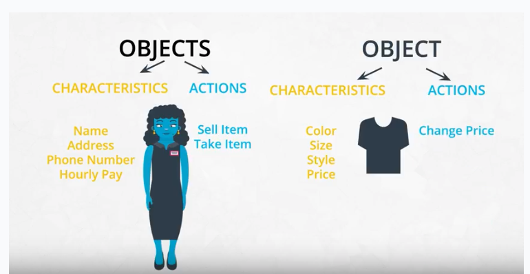
Characteristics and actions in English grammar
You can also think about characteristics and actions is in terms of English grammar. A characteristic corresponds to a noun and an action corresponds to a verb.
Let’s pick something from the real world: a dog. Some characteristics of the dog include the dog’s weight, color, breed, and height. These are all nouns. Some actions a dog can take include to bark, to run, to bite, and to eat. These are all verbs.
Quiz: Characteristics versus actions
Select the characteristics of a tree object. There may be more than one correct answer.
Height
Color
To grow
Width
To fall down
Species
Which of the following would be considered actions for a laptop computer object?
Memory
Width
To turn on
Operating system
To turn off
Thickness
Weight
To erase
Class, object, method, and attribute
Class, object, method, and attribute
Object-oriented programming (OOP) vocabulary
- Class: A blueprint consisting of methods and attributes.
- Object: An instance of a class. It can help to think of objects as something in the real world like a yellow pencil, a small dog, or a blue shirt. However, as you’ll see later in the lesson, objects can be more abstract.
- Attribute: A descriptor or characteristic. Examples would be color, length, size, etc. These attributes can take on specific values like blue, 3 inches, large, etc.
- Method: An action that a class or object could take.
- OOP: A commonly used abbreviation for object-oriented programming.
- Encapsulation: One of the fundamental ideas behind object-oriented programming is called encapsulation: you can combine functions and data all into a single entity. In object-oriented programming, this single entity is called a class.
- Encapsulation allows you to hide implementation details, much like how the
scikit-learnpackage hides the implementation of machine learning algorithms.
In English, you might hear an attribute described as a property, description, feature, quality, trait, or characteristic. All of these are saying the same thing.
Here is a reminder of how a class, an object, attributes, and methods relate to each other.
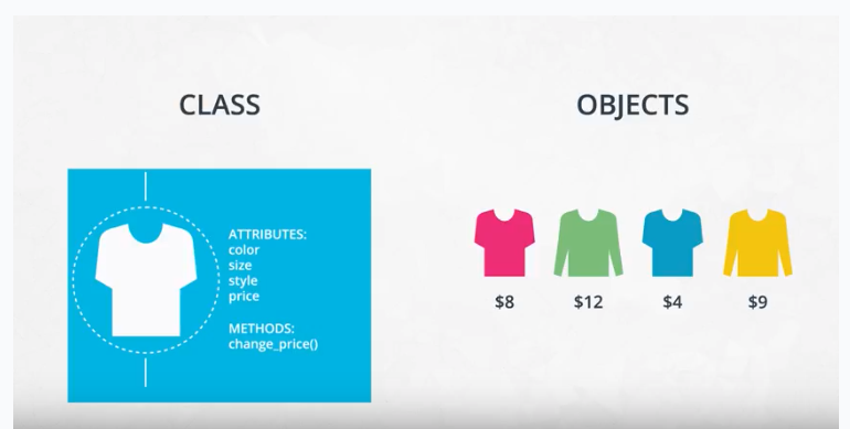
Match the vocabulary term on the left with the examples on the right.
| TERM | EXAMPLES |
|---|---|
| Object | Stephen Hawking, Angela Merkel, Brad Pitt |
| Class | Scientist, chancellor, actor |
| Attribute | Color, size, shape |
| Method | To rain, to ring, to ripen |
| Value | Gray, large, round |
OOP syntax
Object-oriented programming syntax
In this video, you’ll see what a class and object look like in Python. In the next section, you’ll have the chance to play around with the code. Finally, you’ll write your own class.
Function versus method
In the video above, at 1:44, the dialogue mistakenly calls init a function rather than a method. Why is init not a function?
A function and a method look very similar. They both use the def keyword. They also have inputs and return outputs. The difference is that a method is inside of a class whereas a function is outside of a class.
What is self?
If you instantiate two objects, how does Python differentiate between these two objects?
1 | shirt_one = Shirt('red', 'S', 'short-sleeve', 15) |
That’s where self comes into play. If you call the change_price method on shirt_one, how does Python know to change the price of shirt_one and not of shirt_two?
1 | shirt_one.change_price(12) |
Behind the scenes, Python is calling the change_price method:
1 | def change_price(self, new_price): |
Self tells Python where to look in the computer’s memory for the shirt_one object. Then, Python changes the price of the shirt_one object. When you call the change_price method, shirt_one.change_price(12), self is implicitly passed in.
The word self is just a convention. You could actually use any other name as long as you are consistent, but you should use self to avoid confusing people.
Exercise: OOP syntax practice, part 1
Exercise: Use the Shirt class

You’ve seen what a class looks like and how to instantiate an object. Now it’s your turn to write code that instantiates a shirt object.
You need to download three files for this exercise. These files are located on this page in the Supporting materials section.
Shirt_exercise.ipynbcontains explanations and instructions.Answer.pycontaining solution to the exercise.Tests.pytests for checking your code: You can run these tests using the last code cell at the bottom of the notebook.
Getting started
Open the Shirt Exercise.ipynb notebook file using Jupyter Notebook and follow the instructions in the notebook to complete the exercise.
Supporting Materials
Notes about OOP
Notes about OOP
Set and get methods
The last part of the video mentioned that accessing attributes in Python can be somewhat different than in other programming languages like Java and C++. This section goes into further detail.
The Shirt class has a method to change the price of the shirt: shirt_one.change_price(20). In Python, you can also change the values of an attribute with the following syntax:
1 | shirt_one.price = 10 |
This code accesses and changes the price, color, size, and style attributes directly. Accessing attributes directly would be frowned upon in many other languages, but not in Python. Instead, the general object-oriented programming convention is to use methods to access attributes or change attribute values. These methods are called set and get methods or setter and getter methods.
A get method is for obtaining an attribute value. A set method is for changing an attribute value. If you were writing a Shirt class, you could use the following code:
1 | class Shirt: |
Instantiating and using an object might look like the following code:
1 | shirt_one = Shirt('yellow', 'M', 'long-sleeve', 15) |
In the class definition, the underscore in front of price is a somewhat controversial Python convention. In other languages like C++ or Java, price could be explicitly labeled as a private variable. This would prohibit an object from accessing the price attribute directly like shirt_one._price = 15. Unlike other languages, Python does not distinguish between private and public variables. Therefore, there is some controversy about using the underscore convention as well as get and set methods in Python. Why use get and set methods in Python when Python wasn’t designed to use them?
At the same time, you’ll find that some Python programmers develop object-oriented programs using get and set methods anyway. Following the Python convention, the underscore in front of price is to let a programmer know that price should only be accessed with get and set methods rather than accessing price directly with shirt_one._price. However, a programmer could still access _price directly because there is nothing in the Python language to prevent the direct access.
To reiterate, a programmer could technically still do something like shirt_one._price = 10, and the code would work. But accessing price directly, in this case, would not be following the intent of how the Shirt class was designed.
One of the benefits of set and get methods is that, as previously mentioned in the course, you can hide the implementation from your user. Perhaps, originally, a variable was coded as a list and later became a dictionary. With set and get methods, you could easily change how that variable gets accessed. Without set and get methods, you’d have to go to every place in the code that accessed the variable directly and change the code.
You can read more about get and set methods in Python on this Python Tutorial site.
Attributes
There are some drawbacks to accessing attributes directly versus writing a method for accessing attributes.
In terms of object-oriented programming, the rules in Python are a bit looser than in other programming languages. As previously mentioned, in some languages, like C++, you can explicitly state whether or not an object should be allowed to change or access an attribute’s values directly. Python does not have this option.
Why might it be better to change a value with a method instead of directly? Changing values via a method gives you more flexibility in the long-term. What if the units of measurement change, like if the store was originally meant to work in US dollars and now has to handle Euros? Here’s an example:
Example: Dollars versus Euros
If you’ve changed attribute values directly, you’ll have to go through your code and find all the places where US dollars were used, such as in the following:
1 | shirt_one.price = 10 # US dollars |
Then, you’ll have to manually change them to Euros.
1 | shirt_one.price = 8 # Euros |
If you had used a method, then you would only have to change the method to convert from dollars to Euros.
1 | def change_price(self, new_price): |
For the purposes of this introduction to object-oriented programming, you don’t need to worry about updating attributes directly versus with a method; however, if you decide to further your study of object-oriented programming, especially in another language such as C++ or Java, you’ll have to take this into consideration.
Modularized code
Thus far in the lesson, all of the code has been in Jupyter Notebooks. For example, in the previous exercise, a code cell loaded the Shirt class, which gave you access to the shirt class throughout the rest of the notebook.
If you were developing a software program, you would want to modularize this code. You would put the Shirt class into its own Python script, which you might call shirt.py. In another Python script, you would import the Shirt class with a line like from shirt import Shirt.
For now, as you get used to OOP syntax, you’ll be completing exercises in Jupyter Notebooks. Midway through the lesson, you’ll modularize object-oriented code into separate files.
Exercise: OOP syntax practice, part 2
Exercise: Use the Pants class
Now that you’ve had some practice instantiating objects, it’s time to write your own class from scratch.
This lesson has two parts.
- In the first part, you’ll write a
Pantsclass. This class is similar to theShirtclass with a couple of changes. Then you’ll practice instantiatingPantsobjects. - In the second part, you’ll write another class called
SalesPerson. You’ll also instantiate objects for theSalesPerson.
This exercise requires two files, which are located on this page in the Supporting Materials section.
exercise.ipynbcontainsexplanations and instructions.answer.pycontains solution to the exercise.
Getting started
Open the exercise.ipynb notebook file using Jupyter Notebook and follow the instructions in the notebook to complete the exercise.
Supporting Materials
Commenting object-oriented code
Commenting object-oriented code
Did you notice anything special about the answer key in the previous exercise? The Pants class and the SalesPerson class contained docstrings! A docstring is a type of comment that describes how a Python module, function, class, or method works. Docstrings are not unique to object-oriented programming.
For this section of the course, you just need to remember to use docstrings and to comment your code. It will help you understand and maintain your code and even make you a better job candidate.
From this point on, please always comment your code. Use both inline comments and document-level comments as appropriate.
To learn more about docstrings, see Example Google Style Python Docstrings.
Example Google Style Python Docstrings
Example NumPy Style Python Docstrings
Docstrings and object-oriented code
The following example shows a class with docstrings. Here are a few things to keep in mind:
- Make sure to indent your docstrings correctly or the code will not run. A docstring should be indented one indentation underneath the class or method being described.
- You don’t have to define
selfin your method docstrings. It’s understood that any method will haveselfas the first method input.
1 | class Pants: |
Gaussian class
Gaussian class
Resources for review
The example in the next part of the lesson assumes you are familiar with Gaussian and binomial distributions.
Here are a few formulas that might be helpful:
Gaussian distribution formulas
probability density function:
$$\displaystyle f(x | \mu, \sigma^2) = \frac{1}{\sqrt{2\pi\sigma^2}}e^{-(x - \mu)^2/2\sigma^2}$$
- $\mu$ is the mean
- $\sigma$ is the standard deviation
- $\sigma^2$ is the variance
Binomial distribution formulas
- mean: $\displaystyle \mu = n \times p$
In other words, a fair coin has a probability of a positive outcome (heads) $p = 0.5$. If you flip a coin 20 times, the mean would be $20 * 0.5 = 10$; you’d expect to get 10 heads.
- variance: $\displaystyle \sigma^2 = np(1 - p)$
Continuing with the coin example, $n$ would be the number of coin tosses and $p$ would be the probability of getting heads.
- Standard deviation: $\displaystyle \sigma = \sqrt{np(1-p)}$
In other words, the standard deviation is the square root of the variance.
probability density function
$$\displaystyle f(k, n, p) = \frac{n!}{k!(n-k)!}p^k(1-p)^{(n-k)}$$
Further resources
If you would like to review the Gaussian (normal) distribution and binomial distribution, here are a few resources:
This free Udacity course, Intro to Statistics, has a lesson on Gaussian distributions as well as the binomial distribution.
This free course, Intro to Descriptive Statistics, also has a Gaussian distributions lesson.
There are also relevant Wikipedia articles:
Gaussian Distributions Wikipedia
Binomial Distributions Wikipedia
Quiz
How to Use and Create a Z-Table (Standard Normal Table)
Quiz - Gaussian class
Here are a few quiz questions to help you determine how well you understand the Gaussian and binomial distributions. Even if you can’t remember how to answer these types of questions, feel free to move on to the next part of the lesson; however, the material assumes you know what these distributions are and that you know the basics of how to work with them.
Assume the average weight of an American adult male is 180 pounds, with a standard deviation of 34 pounds. The distribution of weights follows a normal distribution. What is the probability that a man weighs exactly 185 pounds?
0.56
0
0.44
0.059
$\mu = 180, \sigma = 34, \sigma^2 = 34^2 = 1156$
Assume the average weight of an American adult male is 180 pounds, with a standard deviation of 34 pounds. The distribution of weights follows a normal distribution. What is the probability that a man weighs somewhere between 120 and 155 pounds?
0
0.23
0.27
0.19
Now, consider a binomial distribution. Assume that 15% of the population is allergic to cats. If you randomly select 60 people for a medical trial, what is the probability that 7 of those people are allergic to cats?
.01
.14
0
.05
.12
How the Gaussian class works
Exercise: Code the Gaussian class
In this exercise, you will use the Gaussian distribution class for calculating and visualizing a Gaussian distribution.
This exercise requires three files, which are located on this page in the Supporting materials section.
Gaussian_code_exercise.ipynbcontains explanations and instructions.Answer.pycontains the solution to the exercise .Numbers.txtcan be read in by theread_data_file()method.
Getting started
Open the Gaussian_code_exercise.ipynb notebook file using Jupyter Notebook and follow the instructions in the notebook to complete the exercise.
Supporting Materials
Magic methods
Magic methods
Magic methods in code
Exercise: Code magic methods
Exercise: Code magic methods
Extend the code from the previous exercise by using two new methods, add and repr.
This exercise requires three files, which are located on this page in the Supporting materials section.
Magic_methods.ipynbcontains explanations and instructions.Answer.pycontains the solution to the exercise.Numbers.txtcan be read in by the read_data_file() method.
Getting started
Open the Magic_methods.ipynb notebook file using Jupyter Notebook and follow the instructions in the notebook to complete the exercise.
Supporting Materials
Inheritance
Inheritance
Inheritance code
In the following video, you’ll see how to code inheritance using Python.
Check the boxes next to the statements that are true. There may be more than one correct answer.
Inheritance helps organize code with a more general version of a class and then specific children.
Inheritance makes code much more difficult to maintain.
Inheritance can make object-oriented programs more efficient to write.
Updates to a parent class automatically trickle down to its children.
Exercise: Inheritance with clothing
Exercise: Inheritance with clothing
Using the Clothing parent class and two children classes, Shirt and Pants, you will code a new class called Blouse.
This exercise requires two files, which are located on this page in the Supporting materials section.
Inheritance_exercise_clothing.ipynbcontains explanations and instructions.Answer.pycontains the solution to the exercise.
Getting started
Open the Inheritance_exercise_clothing.ipynb notebook file using Jupyter Notebook and follow the instructions in the notebook to complete the exercise.
Supporting Materials
Inheritance Gaussian class
Demo: Inheritance probability distributions
Inheritance with the Gaussian class
This is a code demonstration, so you do not need to write any code.
From the Supporting materials section on this page, download the file calledinheritance_probability_distribution.ipynb
Getting started
Open the file using Jupyter Notebook and follow these instructions:
To give another example of inheritance, read through the code in this Jupyter Notebook to see how the code works.
- You can see the Gaussian distribution code is refactored into a generic distribution class and a Gaussian distribution class.
- The distribution class takes care of the initialization and the
read_data_filemethod. The rest of the Gaussian code is in the Gaussian class. You’ll use this distribution class in an exercise at the end of the lesson.
Run the code in each cell of this Jupyter Notebook.
Supporting Materials
Organizing into modules
Organizing into modules
Windows vs. macOS vs. Linux
Linux, which our Udacity classroom workspaces use, is an operating system like Windows or macOS. One important difference is that Linux is free and open source, while Windows is owned by Microsoft and macOS by Apple.
Throughout the lesson, you can do all of your work in a classroom workspace. These workspaces provide interfaces that connect to virtual machines in the cloud. However, if you want to run this code locally on your computer, the commands you use might be slightly different.
If you are using macOS, you can open an application called Terminal and use the same commands that you use in the workspace. That is because Linux and MacOS are related.
If you are using Windows, the analogous application is called Console. The Console commands can be somewhat different than the Terminal commands. Use a search engine to find the right commands in a Windows environment.
The classroom workspace has one major benefit. You can do whatever you want to the workspace, including installing Python packages. If something goes wrong, you can reset the workspace and start with a clean slate; however, always download your code files or commit your code to GitHub or GitLab before resetting a workspace. Otherwise, you’ll lose your code!
Demo: Modularized code
Demo: Modularized code
This is a code demonstration, so you do not need to write any code.
So far, the coding exercises have been in Jupyter Notebooks. Jupyter Notebooks are especially useful for data science applications because you can wrangle data, analyze data, and share a report all in one document. However, they’re not ideal for writing modular programs, which require separating code into different files.
At the bottom of this page under Supporting materials, download three files.
Gaussiandistribution.pyGeneraldistribution.pyexample_code.py
Look at how the distribution class and Gaussian class are modularized into different files.
The Gaussiandistribution.py imports the Distribution class from the Generaldistribution.py file. Note the following line of code:
1 | from Generaldistribution import Distribution |
This code essentially pastes the distribution code to the top of the Gaussiandistribution file when you run the code. You can see in the example_code.py file an example of how to use the Gaussian class.
The example_code.py file then imports the Gaussian distribution class.
For the rest of the lesson, you’ll work with modularized code rather than a Jupyter Notebook. Go through the code in the modularized_code folder to understand how everything is organized.
Supporting Materials
Advanced OOP topics
Inheritance is the last object-oriented programming topic in the lesson. Thus far you’ve been exposed to:
- Classes and objects
- Attributes and methods
- Magic methods
- Inheritance
Classes, object, attributes, methods, and inheritance are common to all object-oriented programming languages.
Knowing these topics is enough to start writing object-oriented software. What you’ve learned so far is all you need to know to complete this OOP lesson. However, these are only the fundamentals of object-oriented programming.
Use the following list of resources to learn more about advanced Python object-oriented programming topics.
- Python’s Instance, Class, and Static Methods Demystified: This article explains different types of methods that can be accessed at the class or object level.
- Class and Instance Attributes: You can also define attributes at the class level or at the instance level.
- Mixins for Fun and Profit: A class can inherit from multiple parent classes.
- Primer on Python Decorators: Decorators are a short-hand way to use functions inside other functions.
Making a package
Making a package
In the previous section, the distribution and Gaussian code was refactored into individual modules. A Python module is just a Python file containing code.
In this next section, you’ll convert the distribution code into a Python package. A package is a collection of Python modules. Although the previous code might already seem like it was a Python package because it contained multiple files, a Python package also needs an __init__.py file. In this section, you’ll learn how to create this __init__.py file and then pip install the package into your local Python installation.
What is pip?
pip is a Python package manager that helps with installing and uninstalling Python packages. You might have used pip to install packages using the command line: pip install numpy. When you execute a command like pip install numpy, pip downloads the package from a Python package repository called PyPI.
For this next exercise, you’ll use pip to install a Python package from a local folder on your computer. The last part of the lesson will focus on uploading packages to PyPi so that you can share your package with the world.
You can complete this entire lesson within the classroom using the provided workspaces; however, if you want to develop a package locally on your computer, you should consider setting up a virtual environment. That way, if you install your package on your computer, the package won’t install into your main Python installation. Before starting the next exercise, the next part of the lesson will discuss what virtual environments are and how to use them.
Object-oriented programming and Python packages
A Python package does not need to use object-oriented programming. You could simply have a Python module with a set of functions. However, most—if not all—of the popular Python packages take advantage of object-oriented programming for a few reasons:
- Object-oriented programs are relatively easy to expand, especially because of inheritance.
- Object-oriented programs obscure functionality from the user. Consider
scipypackages. You don’t need to know how the actual code works in order to use its classes and methods.
Virtual environments
Python environments
In the next part of the lesson, you’ll be given a workspace where you can upload files into a Python package and pip install the package. If you decide to install your package on your local computer, you’ll want to create a virtual environment. A virtual environment is a silo-ed Python installation apart from your main Python installation. That way you can install packages and delete the virtual environment without affecting your main Python installation.
Let’s talk about two different Python environment managers: conda and venv. You can create virtual environments with either one. The following sections describe each of these environment managers, including some advantages and disadvantages. If you’ve taken other data science, machine learning, or artificial intelligence courses at Udacity, you’re probably already familiar with conda.
Conda
Conda does two things: manages packages and manages environments.
As a package manager, conda makes it easy to install Python packages, especially for data science. For instance, typing conda install numpy installs the numpy package.
As an environment manager, conda allows you to create silo-ed Python installations. With an environment manager, you can install packages on your computer without affecting your main Python installation.
The command line code looks something like the following:
1 | conda create --name [environmentname] |
pip and Venv
There are other environmental managers and package managers besides conda. For example, venv is an environment manager that comes preinstalled with Python 3. pip is a package manager.
pip can only manage Python packages, whereas conda is a language agnostic package manager. In fact, conda was invented because pip could not handle data science packages that depended on libraries outside of Python. If you look at the history of conda, you’ll find that the software engineers behind conda needed a way to manage data science packages (such as NumPy and Matplotlib) that relied on libraries outside of Python.
conda manages environments and packages. pip only manages packages.
To use venv and pip, the commands look something like the following:
1 | python3 -m venv [environmentname] |
Which to choose
Whether you choose to create environments with venv or conda will depend on your use case. conda is very helpful for data science projects, but conda can make generic Python software development a bit more confusing; that’s the case for this project.
If you create a conda environment, activate the environment, and then pip install the distributions package, you’ll find that the system installs your package globally rather than in your local conda environment. However, if you create the conda environment and install pip simultaneously, you’ll find that pip behaves as expected when installing packages into your local environment:
1 | conda create --name [environmentname] pip |
On the other hand, using pip with venv works as expected. pip and venv tend to be used for generic software development projects including web development. For this lesson on creating packages, you can use conda or venv if you want to develop locally on your computer and install your package.
The following video shows how to use venv, which is what we recommend for this project.
Instructions for venv
For instructions about how to set up virtual environments on a macOS, Linux, or Windows machine using the terminal, see Installing packages using pip and virtual environments.
Refer to the following notes for understanding the tutorial:
- If you are using Python 2.7.9 or later (including Python 3), the Python installation should already come with the Python package manager called pip. There is no need to install it.
envis the name of the environment you want to create. You can call env anything you want.- Python 3 comes with a virtual environment package preinstalled. Instead of typing
python3 -m virtualenv env, you can typepython3 -m venv envto create a virtual environment.
Once you’ve activated a virtual environment, you can then use terminal commands to go into the directory where your Python library is stored. Then, you can run pip install.
In the next section, you can practice pip installing and creating virtual environments in the classroom workspace. You’ll see that creating a virtual environment actually creates a new folder containing a Python installation. Deleting this folder removes the virtual environment.
If you install packages on the workspace and run into issues, you can always reset the workspace; however, you will lose all of your work. Be sure to download any files you want to keep before resetting a workspace.
Exercise: Making a package and pip installing
Exercise: Making a package and pip installing
In this exercise, you will convert modularized code into a Python package.
This exercise requires three files, which are located on this page in the Supporting materials section.
Gaussiandistribution.pyGeneraldistribution.py3b_answer_python_package.zipcontains the solution to the exercise.
Instructions
Following the instructions from the previous video, convert the modularized code into a Python package.
On your local computer, you need to create a folder called 3a_python_package. Inside this folder, you need to create a few folders and files:
- A
setup.pyfile, which is required in order to usepip install. - A subfolder called
distributions, which is the name of the Python package. - Inside the
distributionsfolder, you need:- The
Gaussiandistribution.pyfile (provided). - The
Generaldistribution.pyfile (provided). - The
__init__.pyfile (you need to create this file).
- The
Once everything is set up, in order to actually create the package, use your terminal window to navigate into the 3a_python_package folder.
Enter the following:
1 | cd 3a_python_package |
If everything is set up correctly, pip installs the distributions package into the workspace. You can then start the Python interpreter from the terminal by entering:
1 | python |
Then, within the Python interpreter, you can use the distributions package by entering the following:
1 | from distributions import Gaussian |
In other words, you can import and use the Gaussian class because the distributions package is now officially installed as part of your Python installation.
If you get stuck, there’s a solution provided in the Supporting materials section called 3b_answer_python_package .
If you want to install the Python package locally on your computer, you might want to set up a virtual environment first. A virtual environment is a silo-ed Python installation apart from your main Python installation. That way you can easily delete the virtual environment without affecting your Python installation.
If you want to try using virtual environments in this workspace first, follow these instructions:
- There is an issue with the Ubuntu operating system and Python3, in which the
venvpackage isn’t installed correctly. In the workspace, one way to fix this is by running this command in the workspace terminal:conda update python. For more information, see venv doesn’t create activate script python3. Then, enterywhen prompted. It might take a few minutes for the workspace to update. If you are not using Anaconda on your local computer, you can skip this first step. - Enter the following command to create a virtual environment:
python -m venv [venv_name]wherevenv_nameis the name you want to give to your virtual environment. You’ll see a new folder appear with the Python installation namedvenv_name. - In the terminal, enter
source venv_name/bin/activate. You’ll notice that the command line now shows(venv_name)at the beginning of the line to indicate you are using thevenv_namevirtual environment. - Enter pip install
python_package/.That should install your distributions Python package. - Try using the package in a program to see if everything works!
Supporting Materials
- Exercise - Making a package and pip installing
- Generaldistribution
- Gaussiandistribution
- 3b Answer Python Package
Binomial class
Binomial class
Binomial class exercise
In the following video, you’ll get an overview of the binomial class exercise.
Exercise: Binomial class
Exercise: Binomial class
In this exercise, you’ll extend the distributions package with a new class called Binomial.
In the Supporting materials section of this page, there is a .zip file called called 4a_binomial_package.zip. Download and unzip this file.
Inside the folder called 4a_binomial_package, there is another folder and these files:
distributions, which contains the code for the distributions package includingGaussiandistribution.pyandGeneraldistribution.pycode.setup.py, a file needed for building Python packages with pip.test.pyunit tests to help you debug your code.numbers.txtandnumbers_binomial.txt, which are data files used as part of the unit tests.Binomialdistribution.pyandBinomialdistribution_challenge.py. Choose one of these files for completing the exercise.Binomialdistribution.pyincludes more of the code already set up for you. In Binomialdistribution_challenge.py, you’ll have to write all of the code from scratch. Both files contain instructions with TODOS to fill out.
In these files, you only need to change the following:
__init__.py, inside the distributions folder. You need to import the binomial package.- Either
Binomialdistribution.pyorBinomialdistribution_challenge.pyYou also need to put yourBinomialdistribution.pyfile into the distributions folder.
When you’re ready to test out your code, follow these steps:
pip install your distributions package. In the terminal, make sure you are in the4a_binomial_packagedirectory. If not, navigate there by entering the following at the command line:
1 | cd 4a_binomial_package |
- Run the unit tests. Enter the following.
1 | python -m unittest test |
Modify the Binomialdistribution.py code until all the unit tests pass.
If you change the code in the distributions folder after pip installing the package, Python will not know about the changes.
When you make changes to the package files, you’ll need to run the following:
1 | pip install --upgrade |
In the Supporting materials section of this page, there is also a solution in the 4b_answer_binomial_package. Try not to look at the solution until your code passes all of the unit tests.
Supporting Materials
scikit-learn source code
scikit-learn source code
Contributing to a GitHub project
Use the following resources to learn how to contribute to a GitHub project:
Advanced Python OOP topics
Use the following resouces to learn about more advanced OOP topics that appear in the scikit-learn package:
Putting code on PyPi
Putting code on PyPi
PyPi vs. test PyPi
Note that pypi.org and test.pypy.org are two different websites. You’ll need to register separately at each website. If you only register at pypi.org , you will not be able to upload to the test.pypy.org repository.
Remember that your package name must be unique. If you use a package name that is already taken, you will get an error when trying to upload the package.
Summary of the terminal commands used in the video
1 | cd binomial_package_files |
More PyPi resources
This tutorial explains how to distribute Python packages, including more configuration options for your setup.py file. You’ll notice that the Python command to run the setup.py is slightly different, as shown in the following example:
1 | python3 setup.py sdist bdist_wheel |
This command still outputs a folder called dist. The difference is that you will get both a .tar.gz file and a .whl file. The .tar.gz file is called a source archive, whereas the .whl file is a built distribution. The .whl file is a newer type of installation file for Python packages. When you pip install a package, pip firsts look for a .whl file (wheel file); if there isn’t one, it looks for the .tar.gz file.
A .tar.gz file (an sdist) contains the files needed to compile and install a Python package. A .whl file (a built distribution) only needs to be copied to the proper place for installation. Behind the scenes, pip installing a .whl file has fewer steps than installing a .tar.gz file.
Other than this command, the rest of the steps for uploading to PyPi are the same.
Other Links
To learn more about PyPi, see the following resources:
Exercise: Upload to PyPi
Exercise: Upload to PyPi
In this part of the lesson, you’ll practice uploading a package to PyPi.
In the Supporting materials section of this page, there is a zip file called 5_exercise_upload_to_pypi.zip . Download and unzip this file.
The Python package is located in the folder 5_exercise_upload_to_pypi.
You need to create three files:
setup.cfgREADME.mdlicense.txt
You also need to create accounts for the pypi test repository and pypi repository.
Don’t forget to keep your passwords; you’ll need to type them into the command line.
Once you have all the files set up correctly, you can use the following commands on the command line. You need to make the name of the package unique, so change the name of the package from distributions to something else. That means changing the information in setup.py and the folder name.
In the terminal, make sure you are in the 5_exercise_upload_to_pypi directory. If not, navigate there by entering the following at the command line:
1 | cd 5_exercise_upload_to_pypi |
Commands to upload to the PyPi test repository
1 | twine upload --repository-url https://test.pypi.org/legacy/ dist/* |
Command to upload to the PyPi repository
1 | twine upload dist/* |
If you get stuck, rewatch the previous video showing how to upload a package to PyPi.
Supporting Materials
Lesson summary
What we covered in this lesson
- Classes vs. objects
- Methods and attributes
- Magic methods and inheritance
- Python packages
Resources
Projects URL
Programming
Writing READMEs
Introduction to Python Programming
Example Google Style Python Docstrings
Example NumPy Style Python Docstrings
Python, Memory, and Objects
Advanced OOP
Python’s Instance, Class, and Static Methods Demystified: This article explains different types of methods that can be accessed at the class or object level.
Class and Instance Attributes: You can also define attributes at the class level or at the instance level.
Mixins for Fun and Profit: A class can inherit from multiple parent classes.
Primer on Python Decorators: Decorators are a short-hand way to use functions inside other functions.
Decorators
Git
A successful Git branching model
Version Control with Git
About merge conflicts
How to version control your production machine learning models
Version Control ML Model
GitHub
Beginner’s Guide to Contributing to a Github Project
Contributing to a Github Project
Machine Learning
Introduction to Machine Learning Course
Intro to TensorFlow for Deep Learning
Intro to Deep Learning with PyTorch
Neural networks - 3Blue1Bro
Math
Intro to Statistics
Intro to Descriptive Statistics
Mathematics for Machine Learning: Linear Algebra
Linear Algebra Courses (edX)
Linear Algebra by MIT (OCW MIT)
Essence of linear algebra - - 3Blue1Bro
AWS