AWS SageMaker Lab
AWS SageMaker
SageMaker
Build a Custom GAN Model
https://github.com/aws-samples/aws-deepcomposer-samples
https://github.com/aws-samples/aws-deepcomposer-samples/blob/master/gan/GAN.ipynb
https://github.com/aws-samples/aws-deepcomposer-samples/tree/master/gan
SageMaker Configuration
Services -> SageMaker -> -> Notebook -> Notebook instances
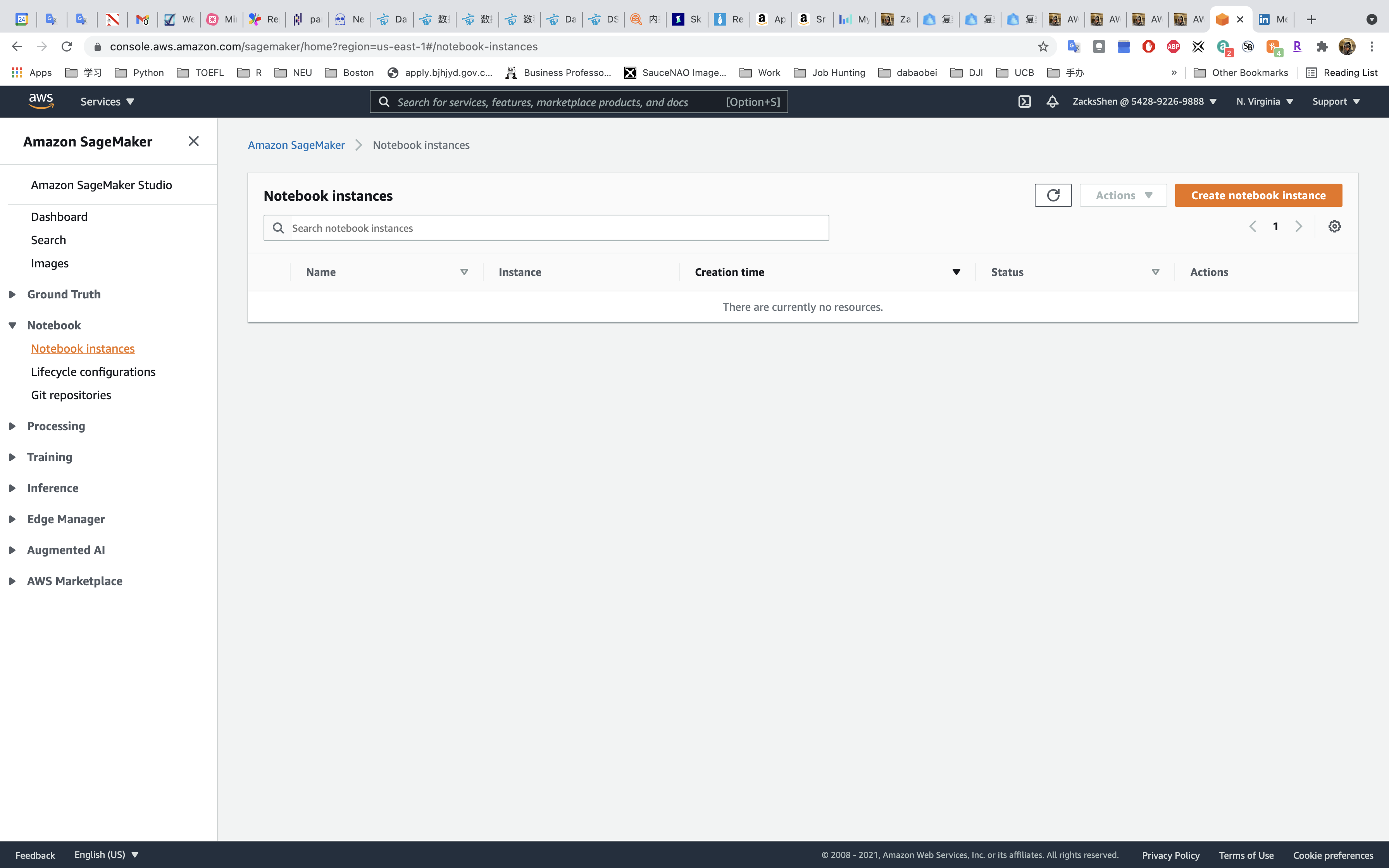
Click on Create notebook instances
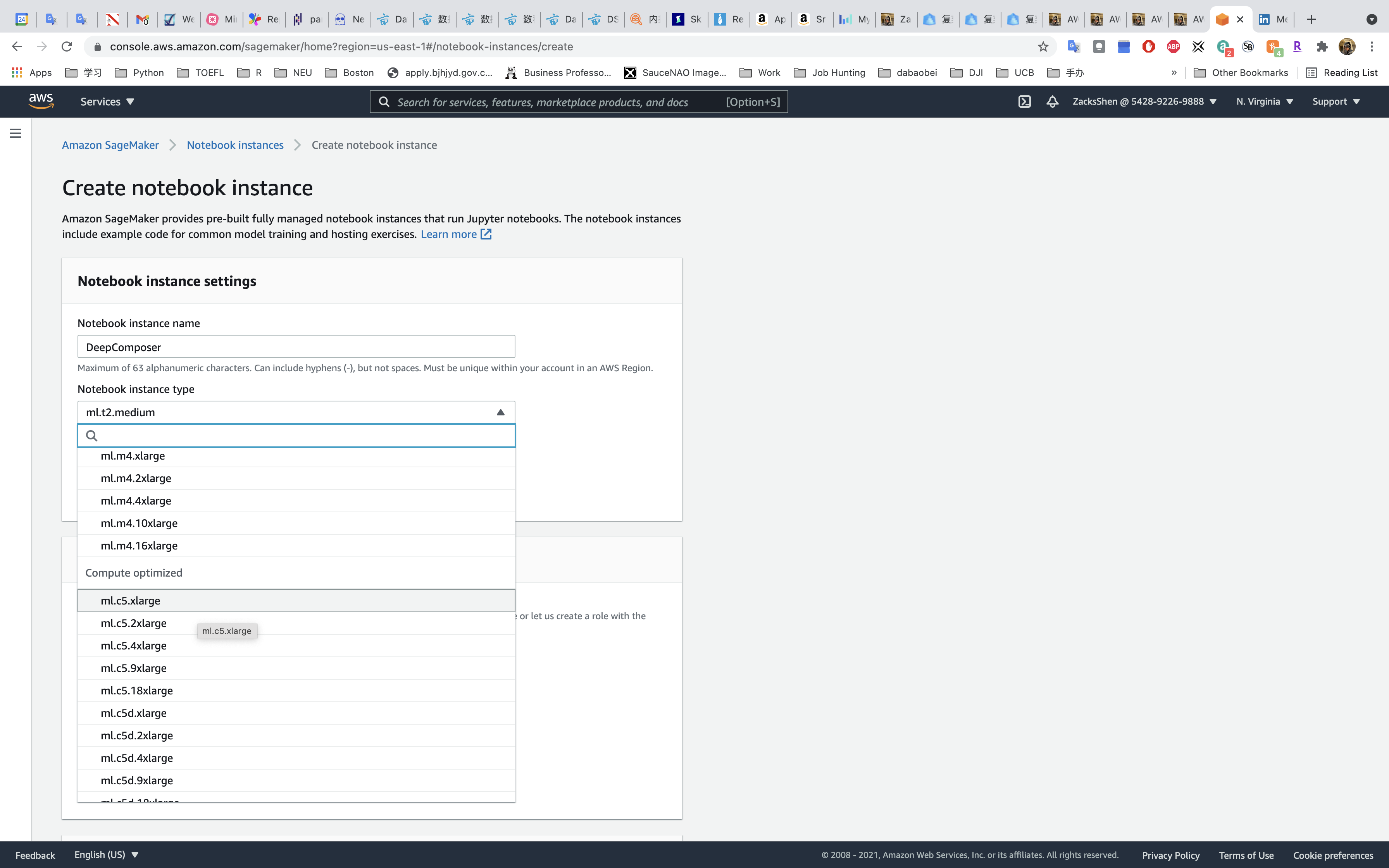
Notebook instance settings
- Notebook instance name: any
- Notebook instance type:
ml.c5.4xlarge- Based on the kind of CPU, GPU and memory you need the next step is to select an instance type. For our purposes, we’ll configure a powerful instance (not covered in the Amazon SageMaker free tier)
- Elastic Inference:
none
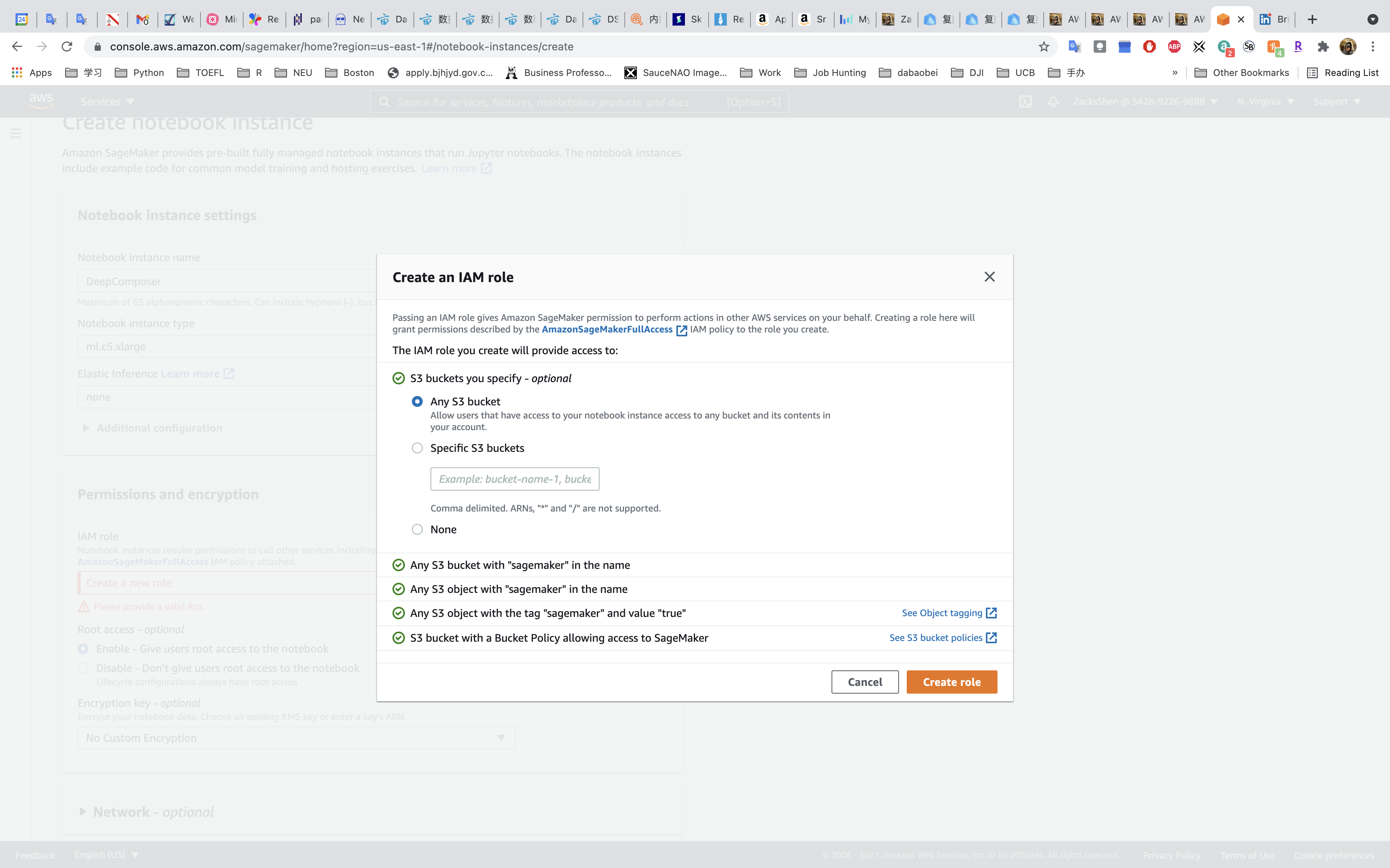
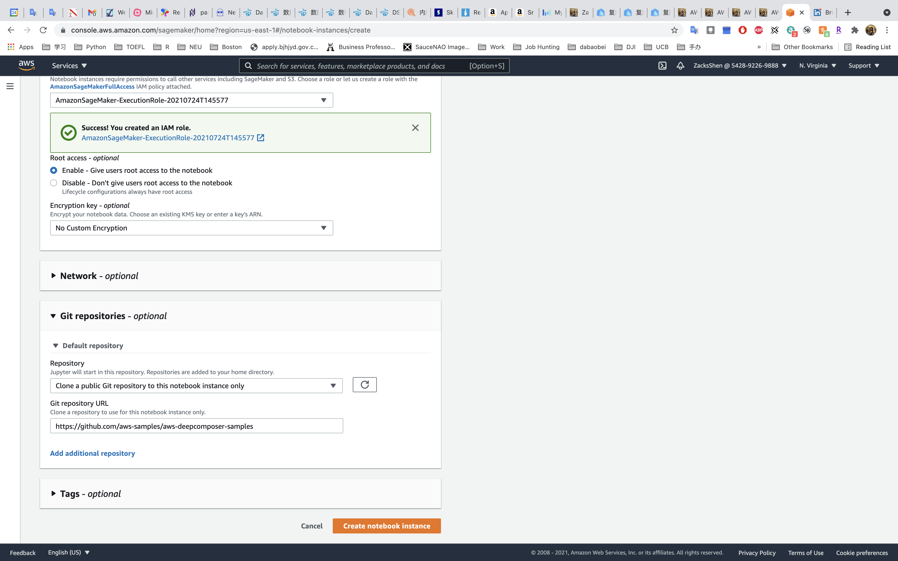
Permissions and encryption
- IAM role:
Create a new roleand leave everything default.
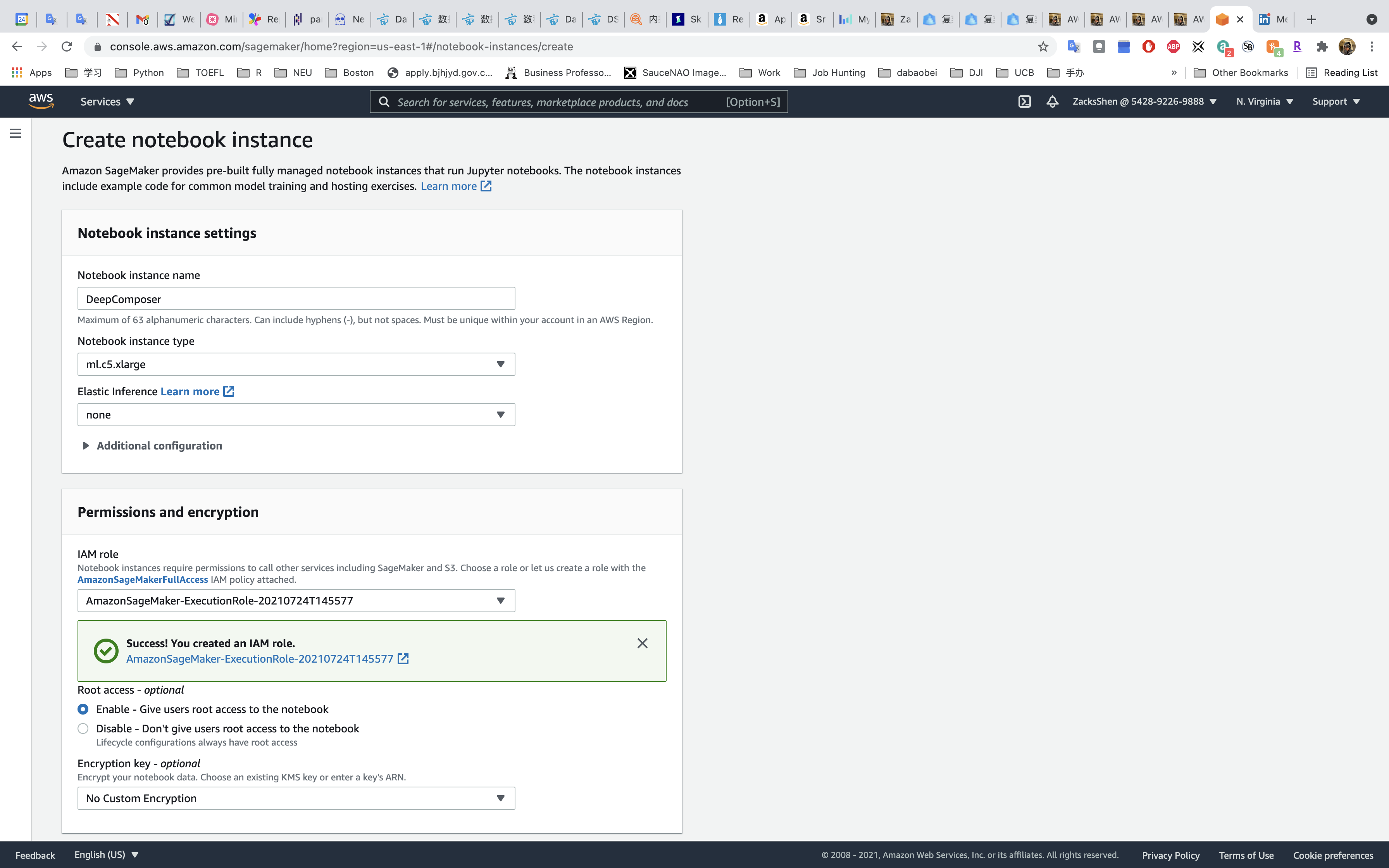
Git repositories
- Repository:
Clone a public Git repository to this notebook instance only - Git repository UR:
https://github.com/aws-samples/aws-deepcomposer-samples
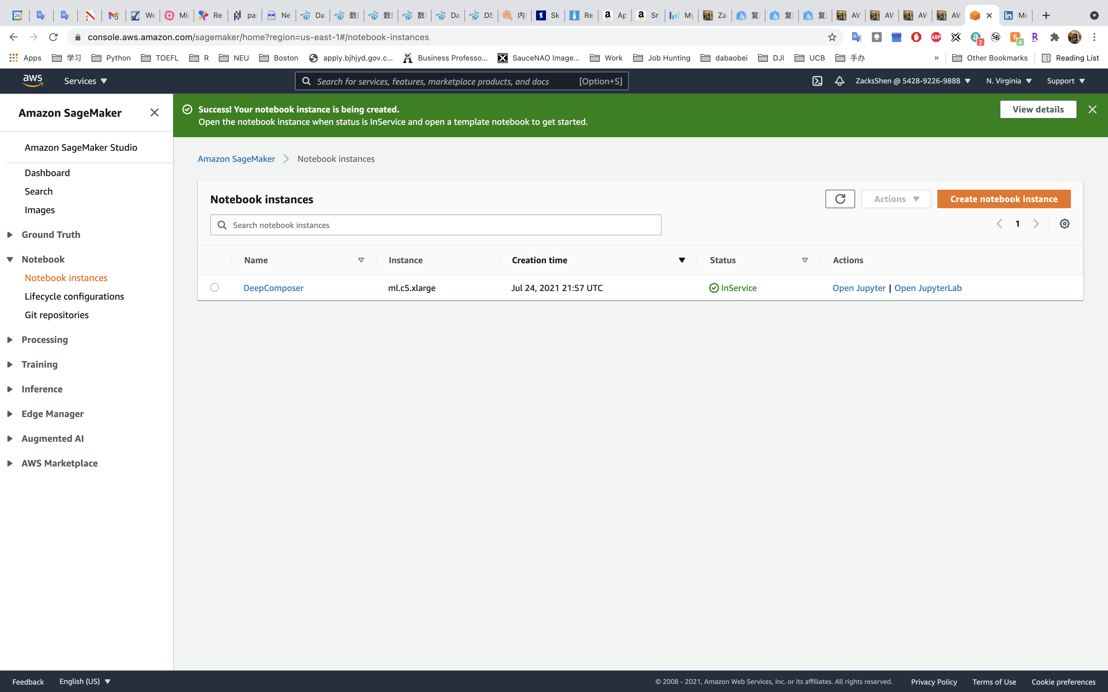
Click on Create notebook instance
Give SageMaker a few minutes to provision the instance and clone the Git repository
When the status reads “InService” you can open the Jupyter notebook.
Notebook Configuration
Click on Open Jupyter
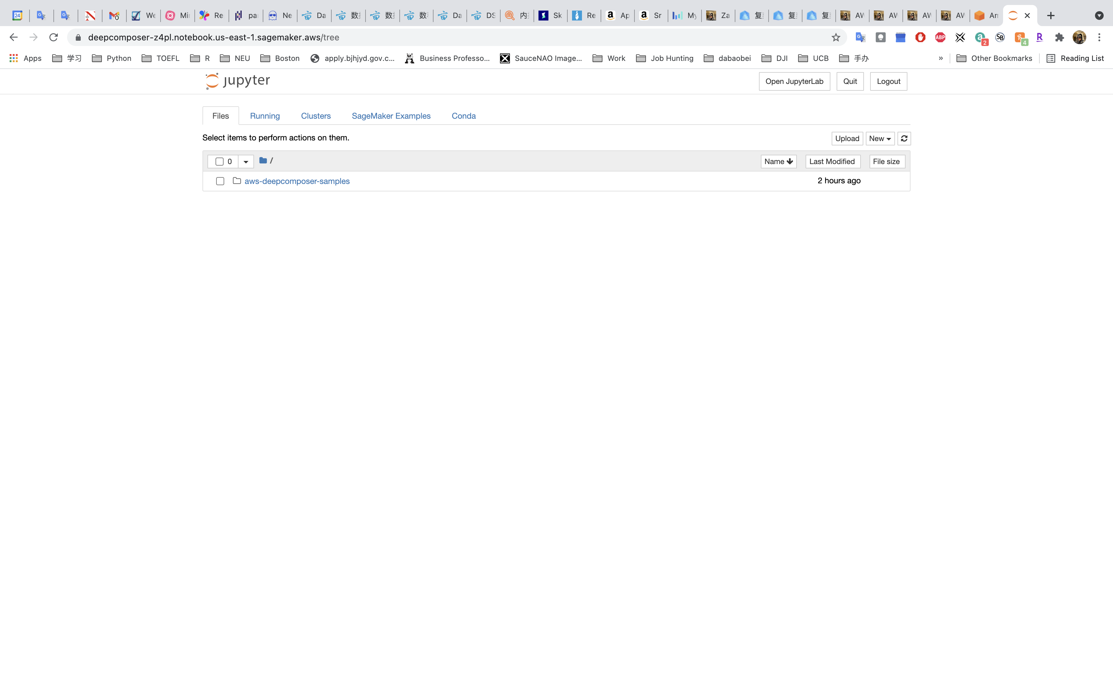
Click on aws-deepcomposer-samples.
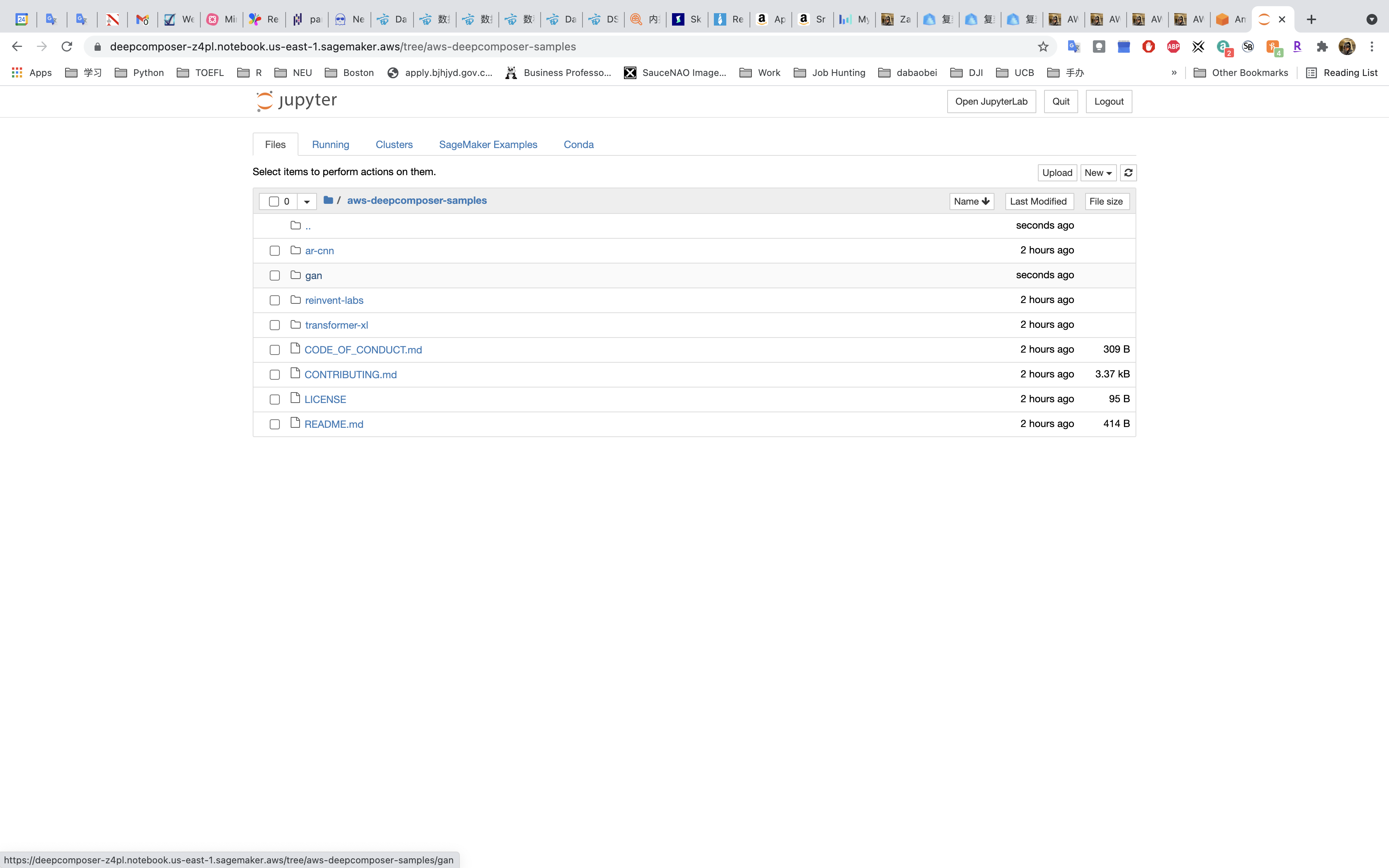
Click on gan.
Click on GAN.ipynb on the left panel.
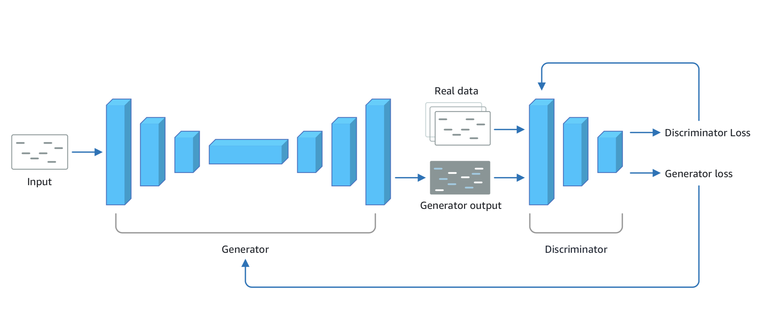
Review: Generative Adversarial Networks (GANs).
GANs consist of two networks constantly competing with each other:
- Generator network that tries to generate data based on the data it was trained on.
- Discriminator network that is trained to differentiate between real data and data which is created by the generator.
Project
Dependencies
Run the first Dependencies cell to install the required packages
The followings are required packages:
https://github.com/aws-samples/aws-deepcomposer-samples/blob/master/gan/requirements.sh
1 |
|
source activate python3is the command for loading local Python environment.conda update --all --yis the command for updating all of the Conda packages.
Wait until All the required packages are installed successfully...
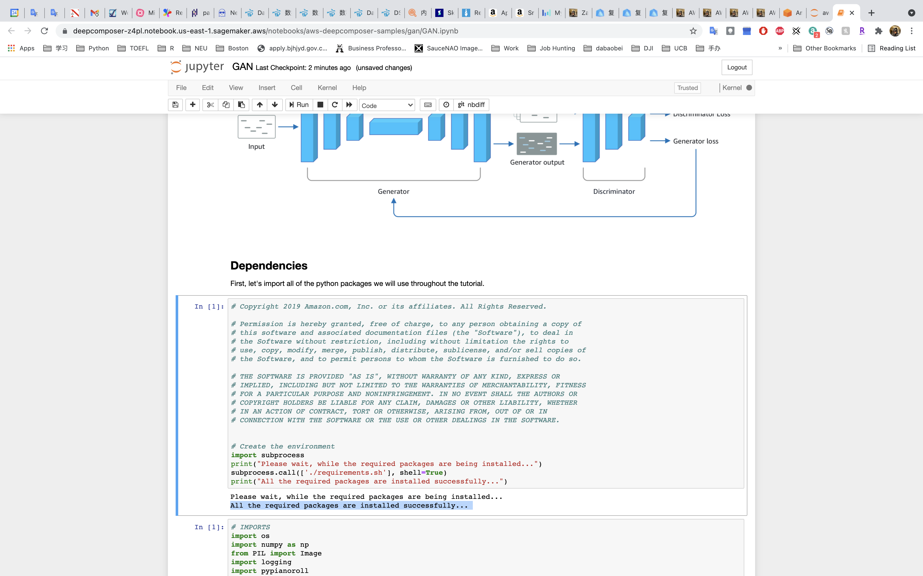
Import the packages.
Configuration
Good Coding Practices
- Do not hard-code configuration variables
- Move configuration variables to a separate
configfile - Use code comments to allow for easy code collaboration
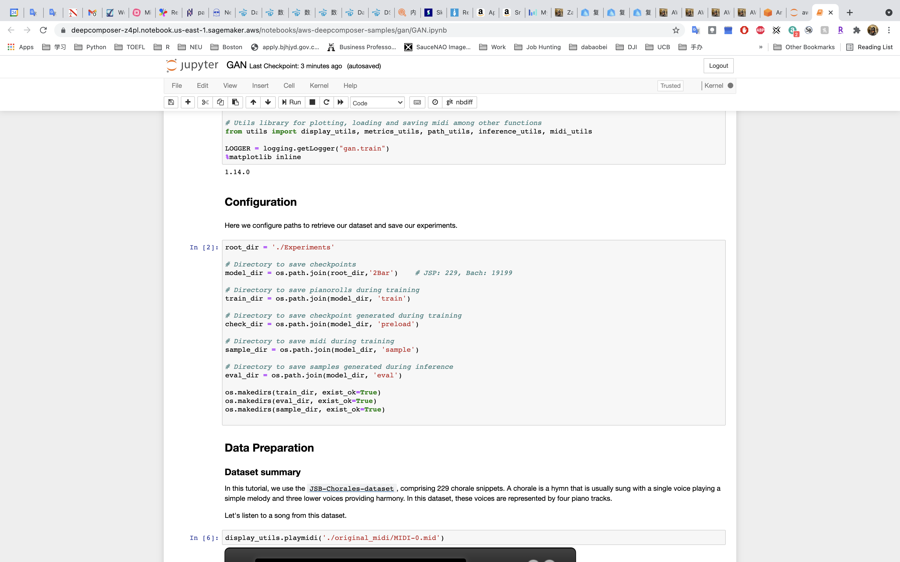
In the Configuration part, we set the following variables:
root_dirmodel_dirtrain_dircheck_dirsample_direval_dir
Data Preparation
The next section of the notebook is where we’ll prepare the data so it can train the generator network.
Why Do We Need to Prepare Data?
Data often comes from many places (like a website, IoT sensors, a hard drive, or physical paper) and it’s usually not clean or in the same format. Before you can better understand your data, you need to make sure it’s in the right format to be analyzed. Thankfully, there are library packages that can help! One such library is called NumPy, which was imported into our notebook.
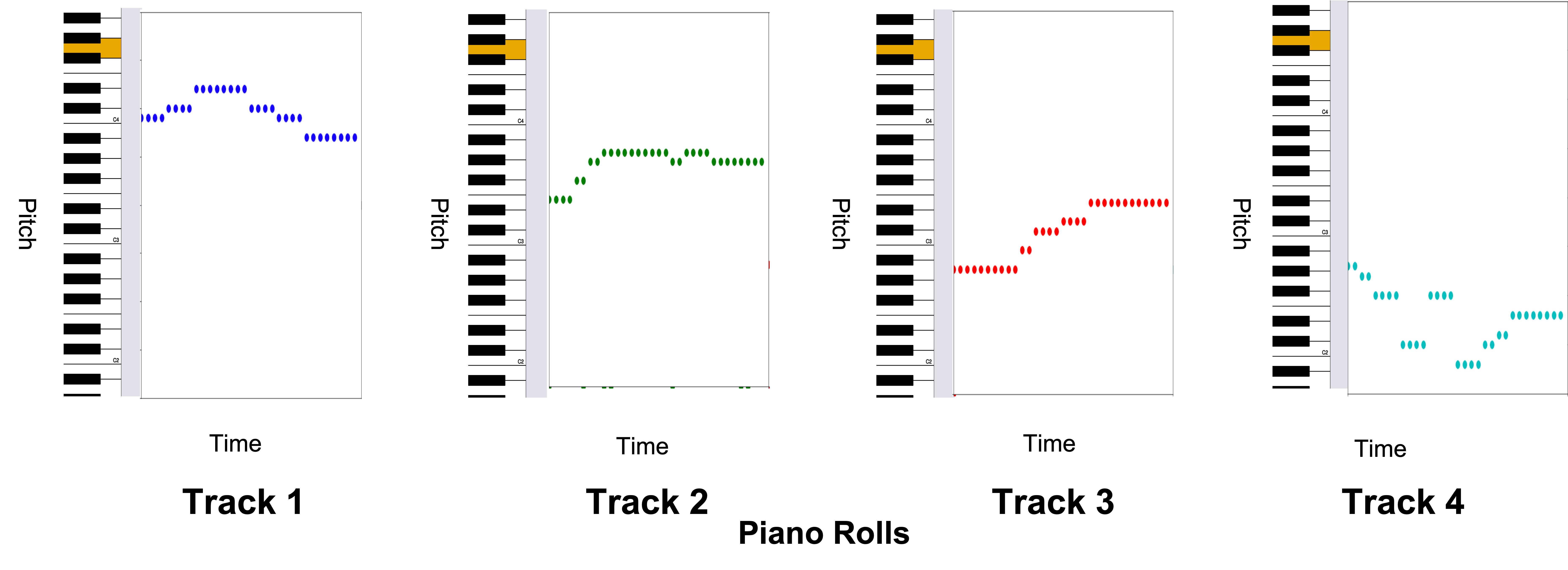
Piano Roll Format
The data we are preparing today is music and it comes formatted in what’s called a “piano roll”. Think of a piano roll as a 2D image where the X-axis represents time and the Y-axis represents the pitch value. Using music as images allows us to leverage existing techniques within the computer vision domain.
Our data is stored as a NumPy Array, or grid of values. Our dataset comprises 229 samples of 4 tracks (all tracks are piano). Each sample is a 32 time-step snippet of a song, so our dataset has a shape of:
1 | (num_samples, time_steps, pitch_range, tracks) |
or
1 | (229, 32, 128, 4) |
Run the next cell to play a song from the dataset.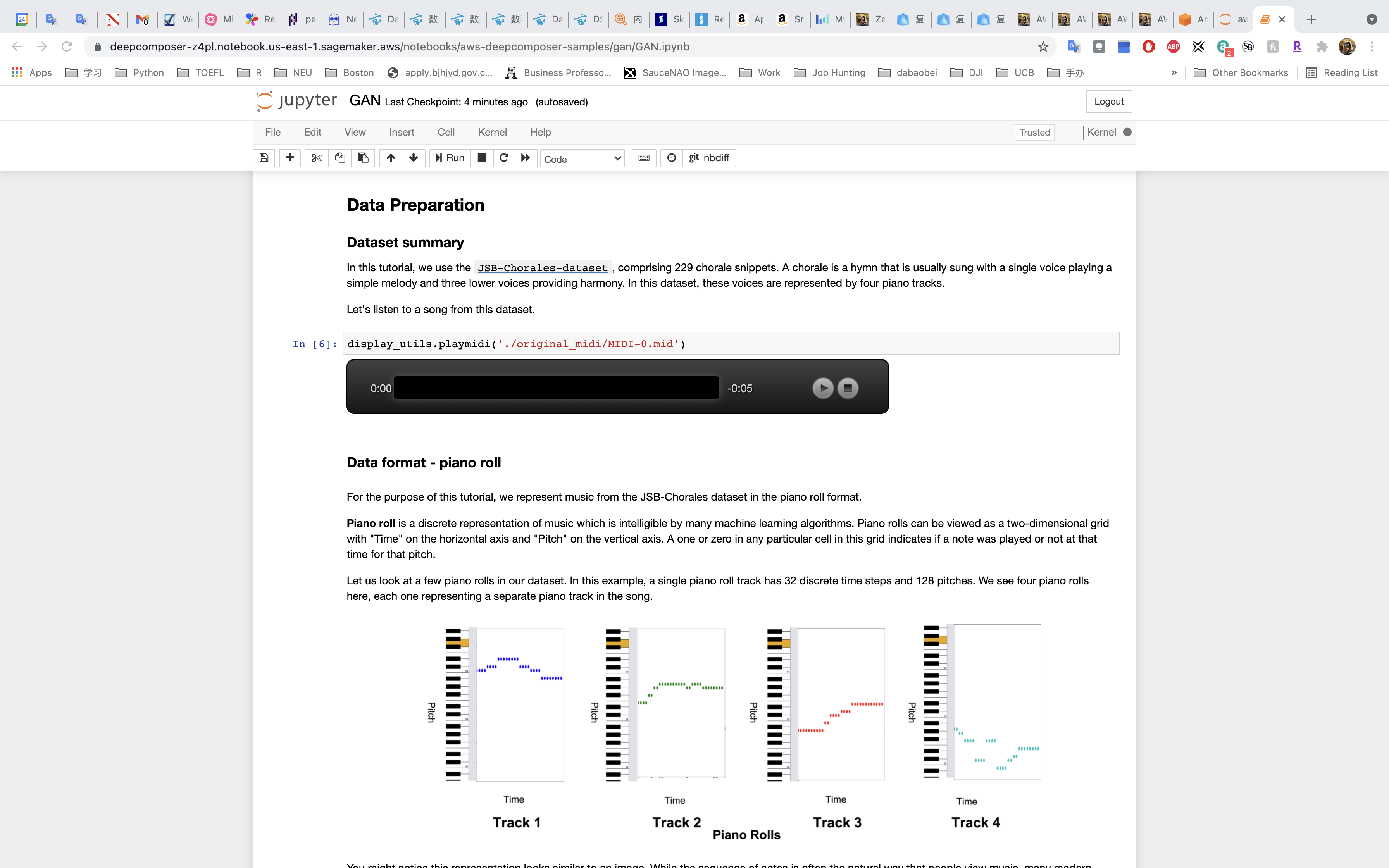
Run the next cell to load the dataset as a nympy array and output the shape of the data to confirm that it matches the (229, 32, 128, 4) shape we are expecting
Run the next cell to see a graphical representation of the data.
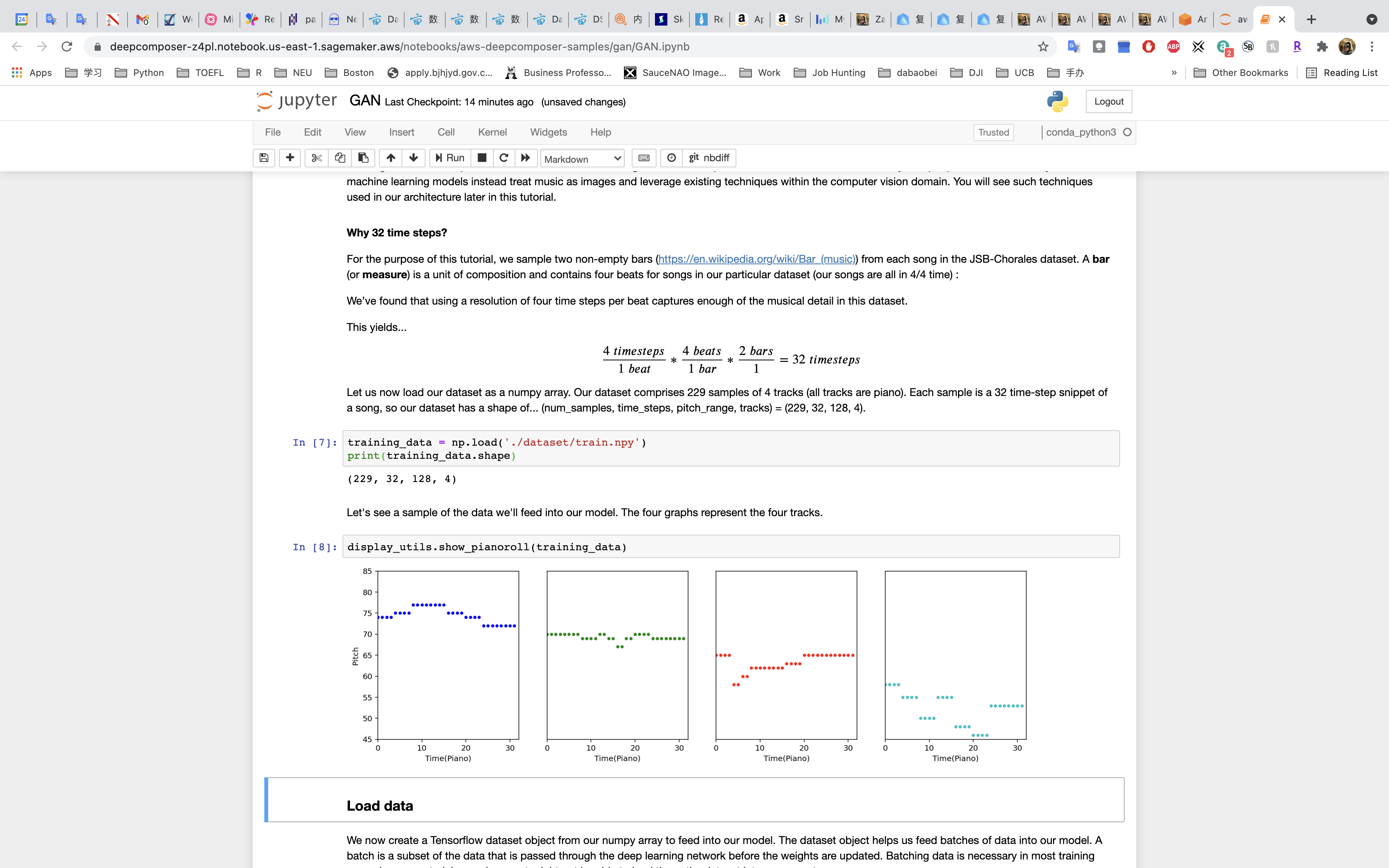
Create a Tensorflow Dataset
Much like there are different libraries to help with cleaning and formatting data, there are also different frameworks. Some frameworks are better suited for particular kinds of machine learning workloads and for this deep learning use case, we’re going to use a Tensorflow framework with a Keras library.
We’ll use the dataset object to feed batches of data into our model.
Run the first Load Data cell to set parameters.
Run the second Load Data cell to prepare the data.
Model Architecture
Before we can train our model, let’s take a closer look at model architecture including how GAN networks interact with the batches of data we feed into the model, and how the networks communicate with each other.
How the Model Works
The model consists of two networks, a generator and a discriminator (critic). These two networks work in a tight loop:
- The generator takes in a batch of single-track piano rolls (melody) as the input and generates a batch of multi-track piano rolls as the output by adding accompaniments to each of the input music tracks.
- The discriminator evaluates the generated music tracks and predicts how far they deviate from the real data in the training dataset.
- The feedback from the discriminator is used by the generator to help it produce more realistic music the next time.
- As the generator gets better at creating better music and fooling the discriminator, the discriminator needs to be retrained by using music tracks just generated by the generator as fake inputs and an equivalent number of songs from the original dataset as the real input.
- We alternate between training these two networks until the model converges and produces realistic music.
The discriminator is a binary classifier which means that it classifies inputs into two groups, e.g. “real” or “fake” data.
Defining and Building Our Model
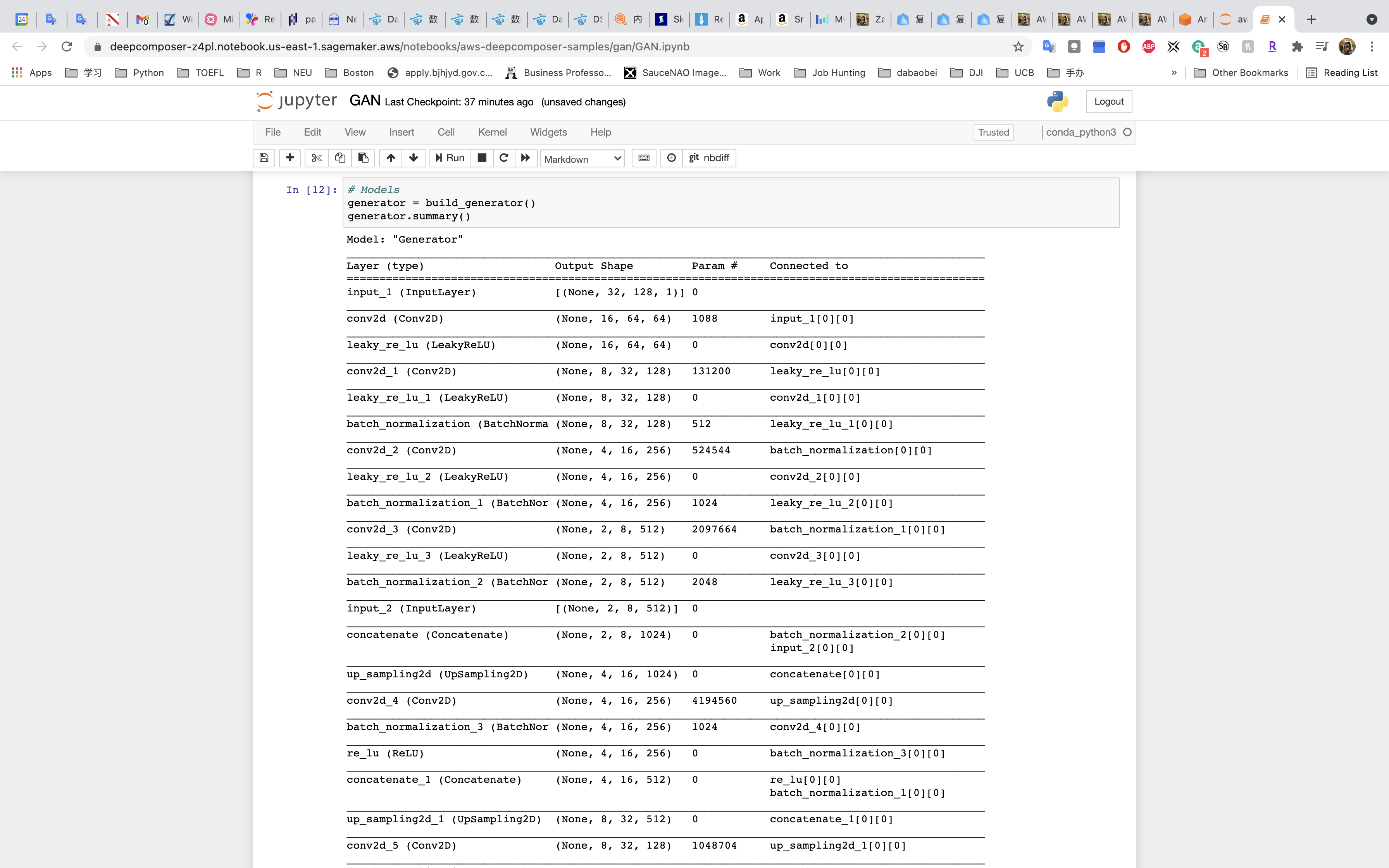
Run the cell that defines the generator
Run the cell that builds the generator
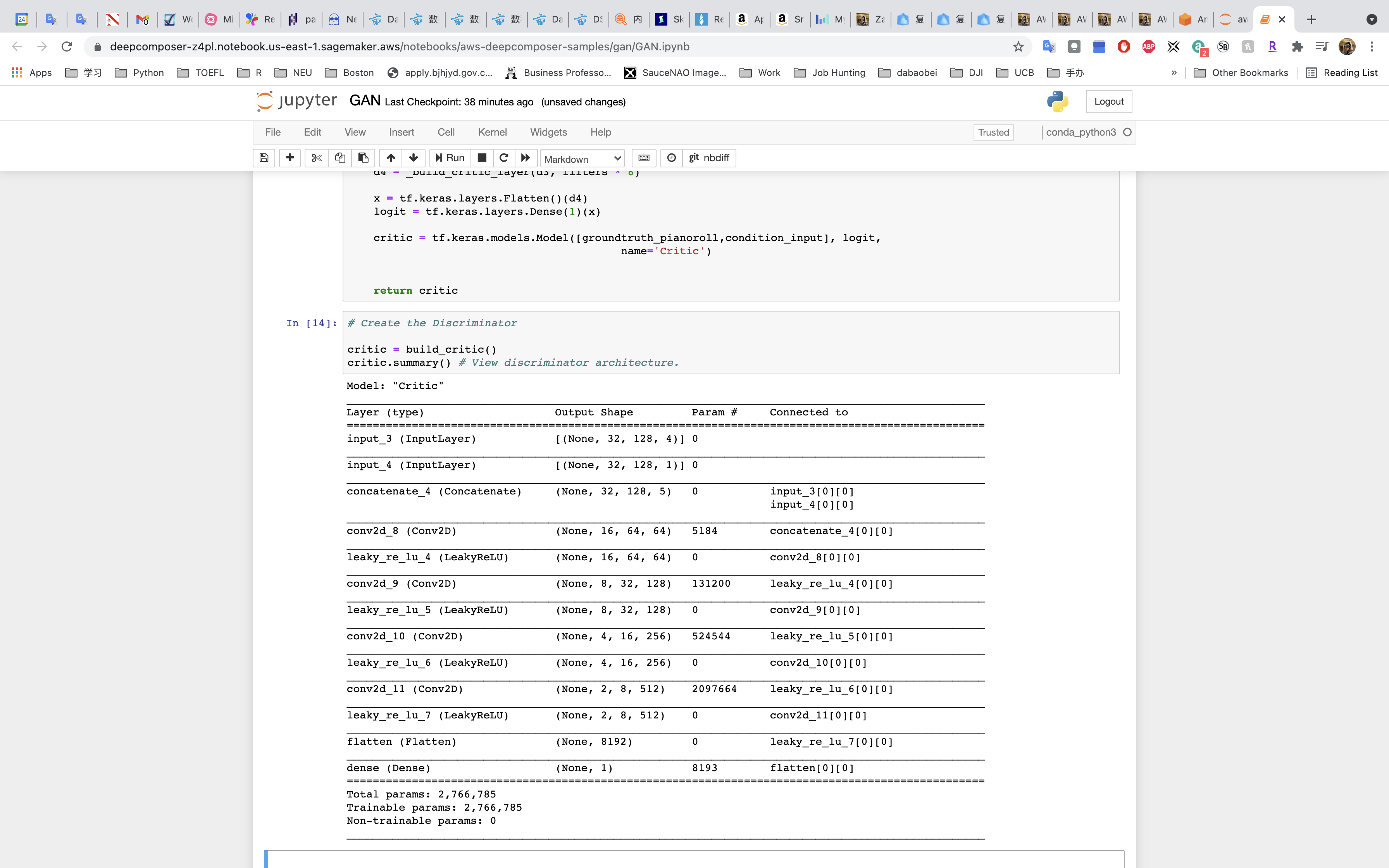
Run the cell that defines the discriminator
Run the cell that builds the discriminator
Model Training and Loss Functions
As the model tries to identify data as “real” or “fake”, it’s going to make errors. Any prediction different than the ground truth is referred to as an error.
The measure of the error in the prediction, given a set of weights, is called a loss function. Weights represent how important an associated feature is to determining the accuracy of a prediction.
Loss functions are an important element of training a machine learning model because they are used to update the weights after every iteration of your model. Updating weights after iterations optimizes the model making the errors smaller and smaller.
Setting Up and Running the Model Training
Run the cell that defines the loss functions
Run the cell to set up the optimizer
Run the cell to define the generator step function
Run the cell to define the discriminator step function
Run the cell to load the melody samples
Run the cell to set the parameters for the training
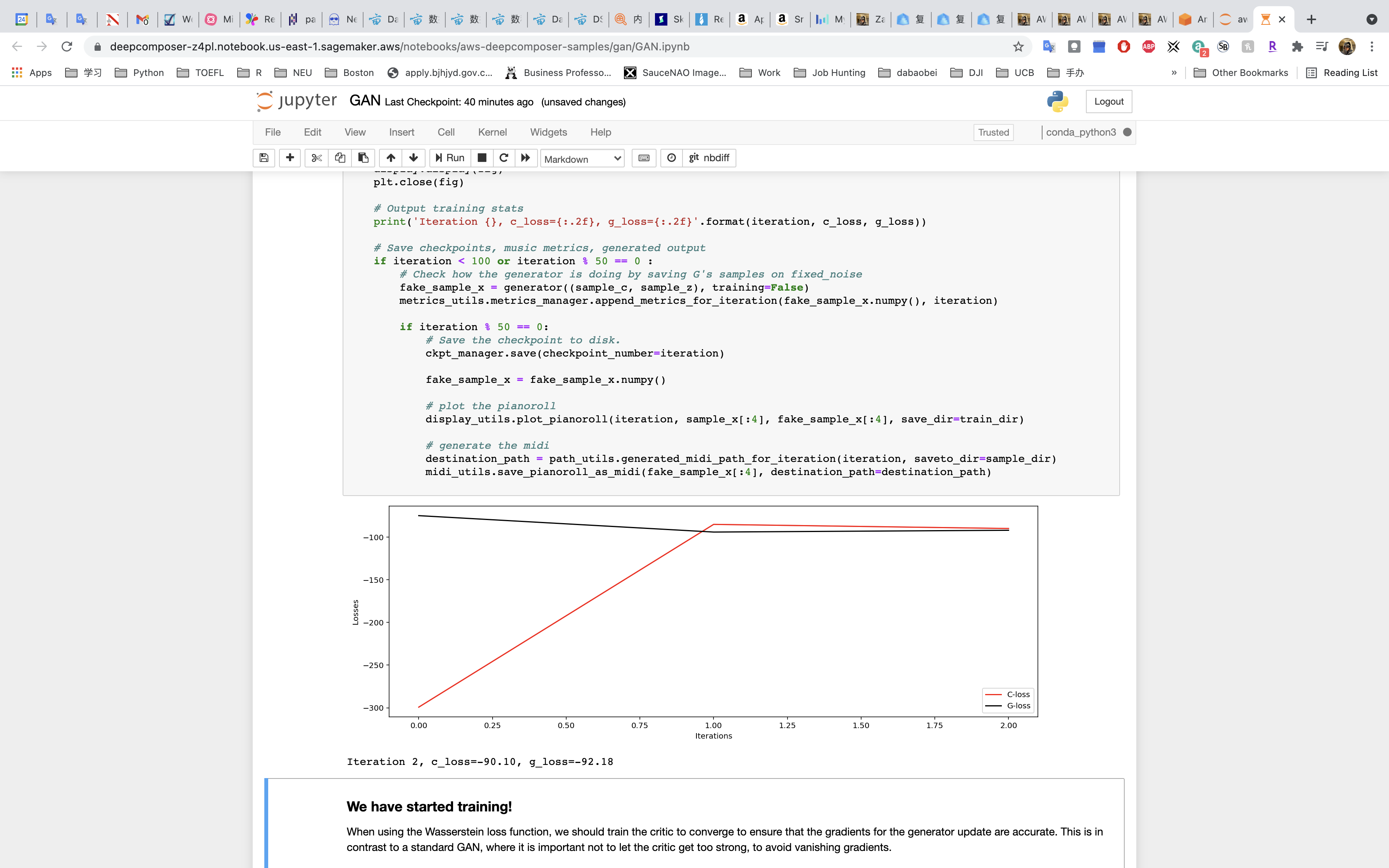
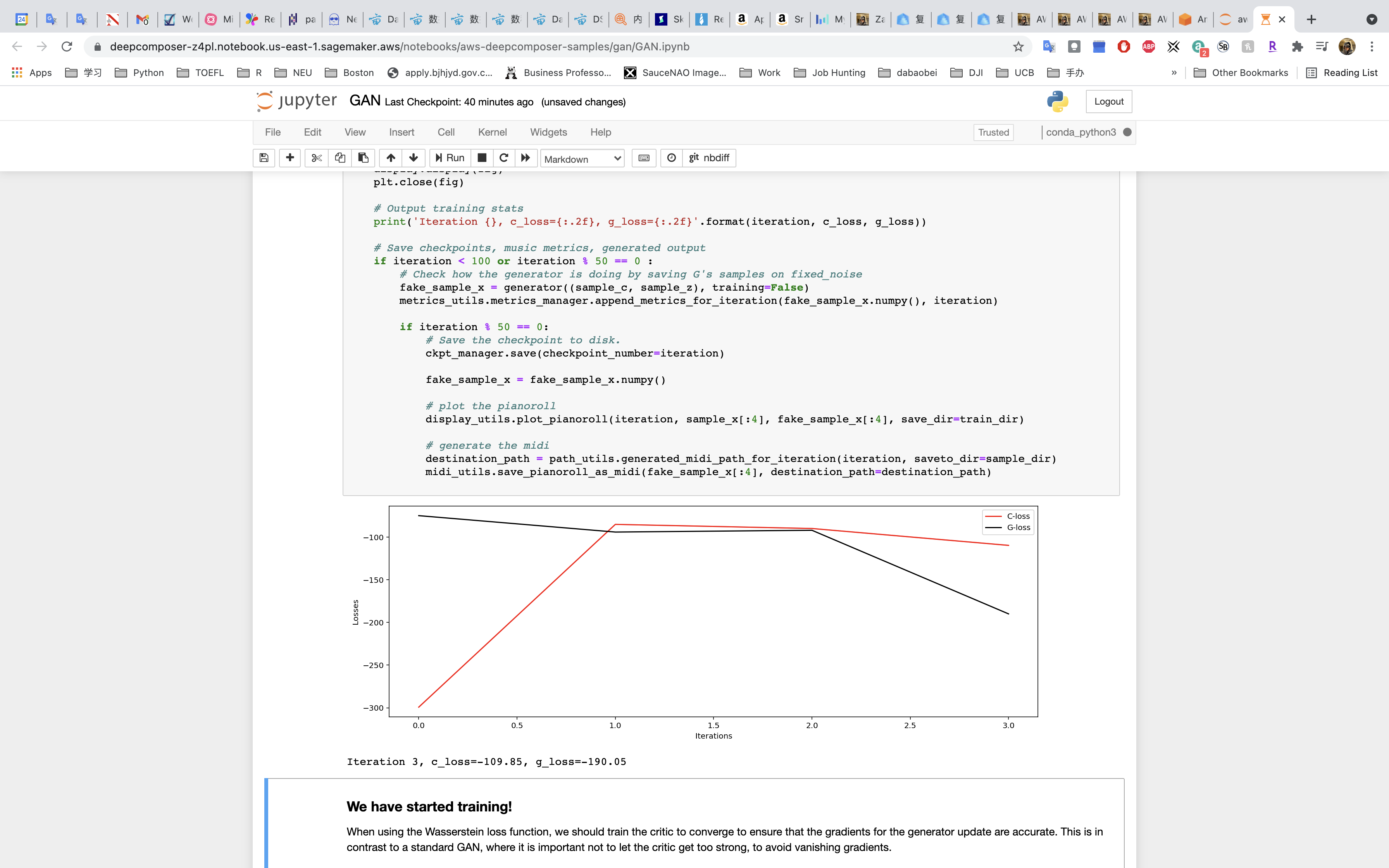
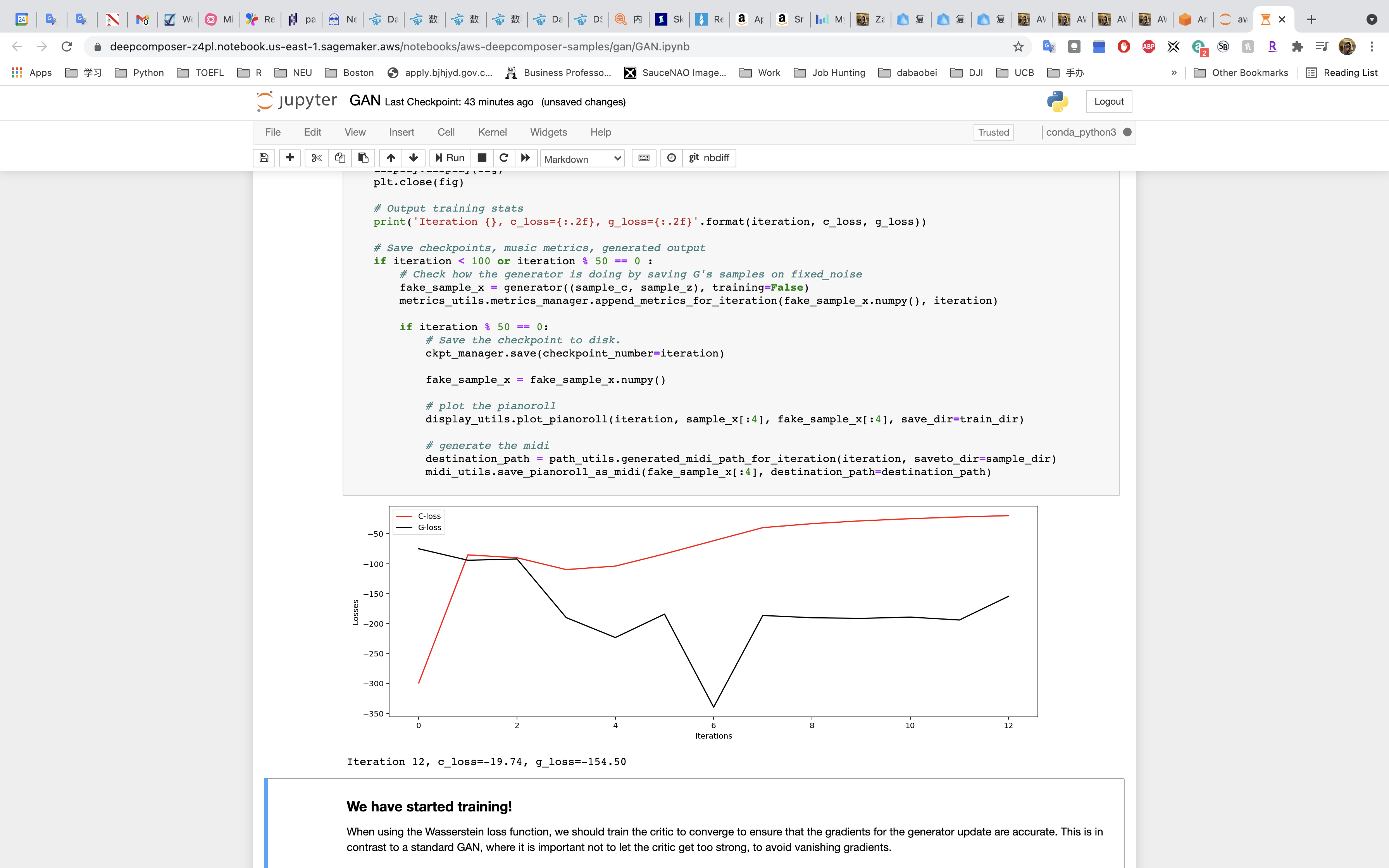
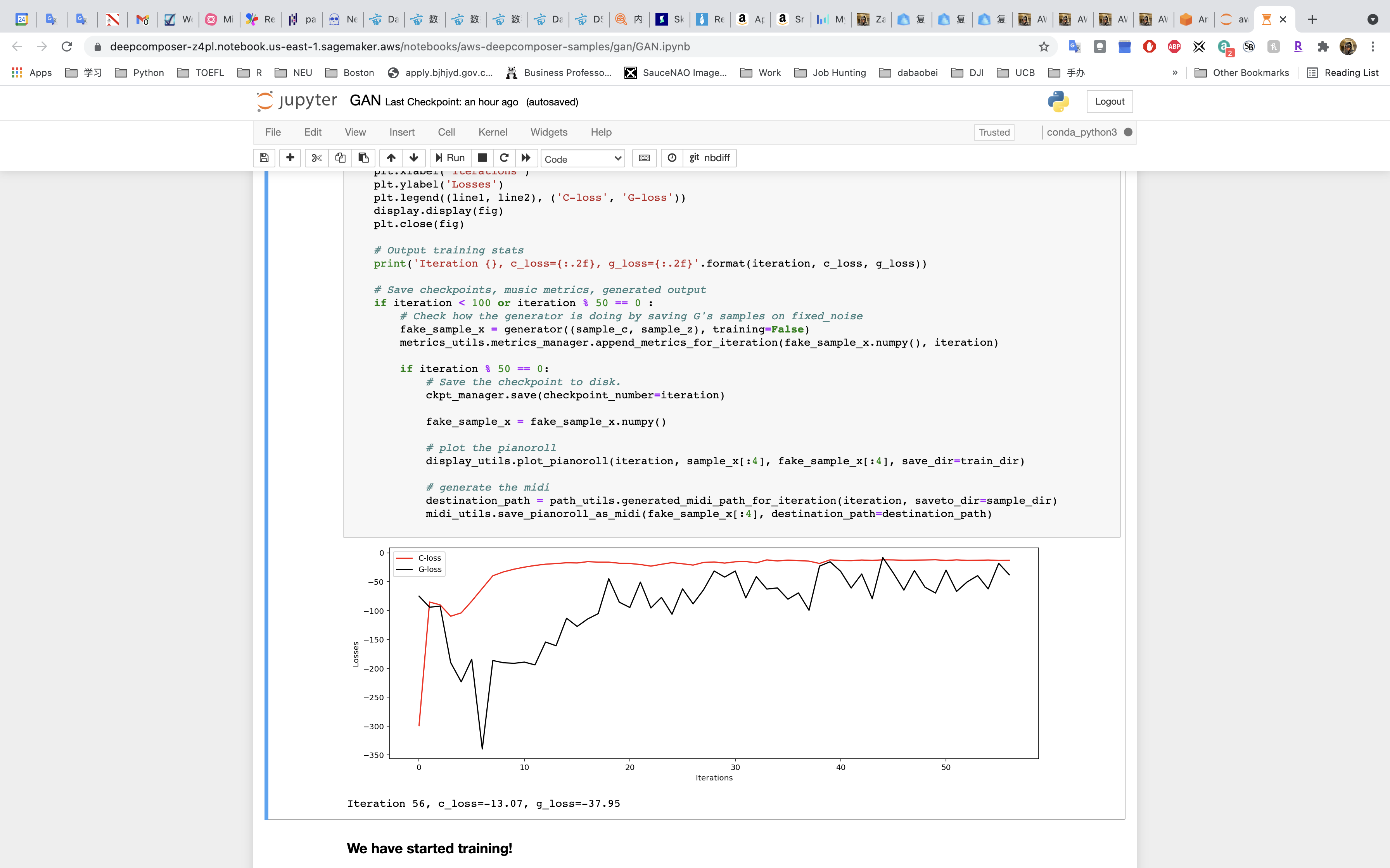
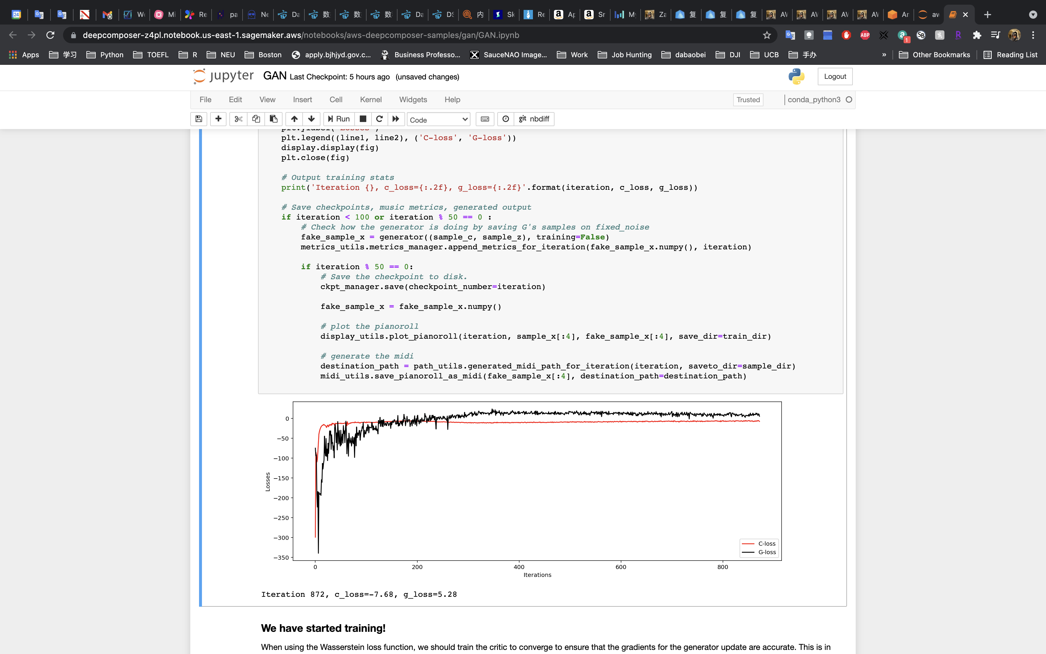
Run the cell to train the model!!!!
Training and tuning models can take a very long time – weeks or even months sometimes. Our model will take around an hour to train.
Model Evaluation
Now that the model has finished training it’s time to evaluate its results.
There are several evaluation metrics you can calculate for classification problems and typically these are decided in the beginning phases as you organize your workflow.
You can:
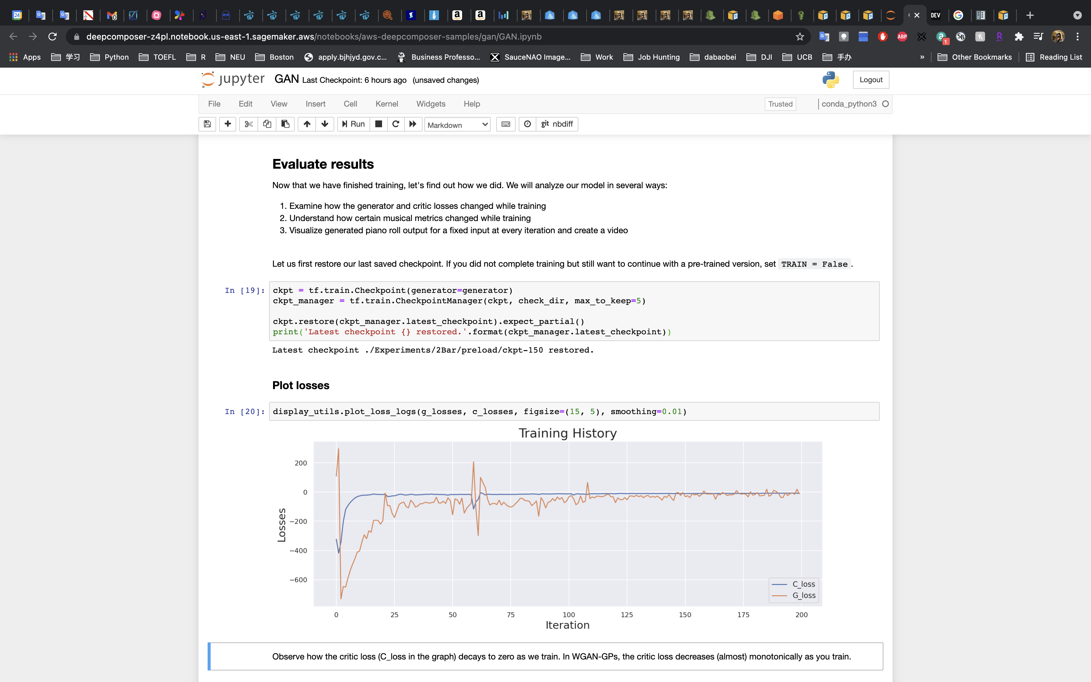
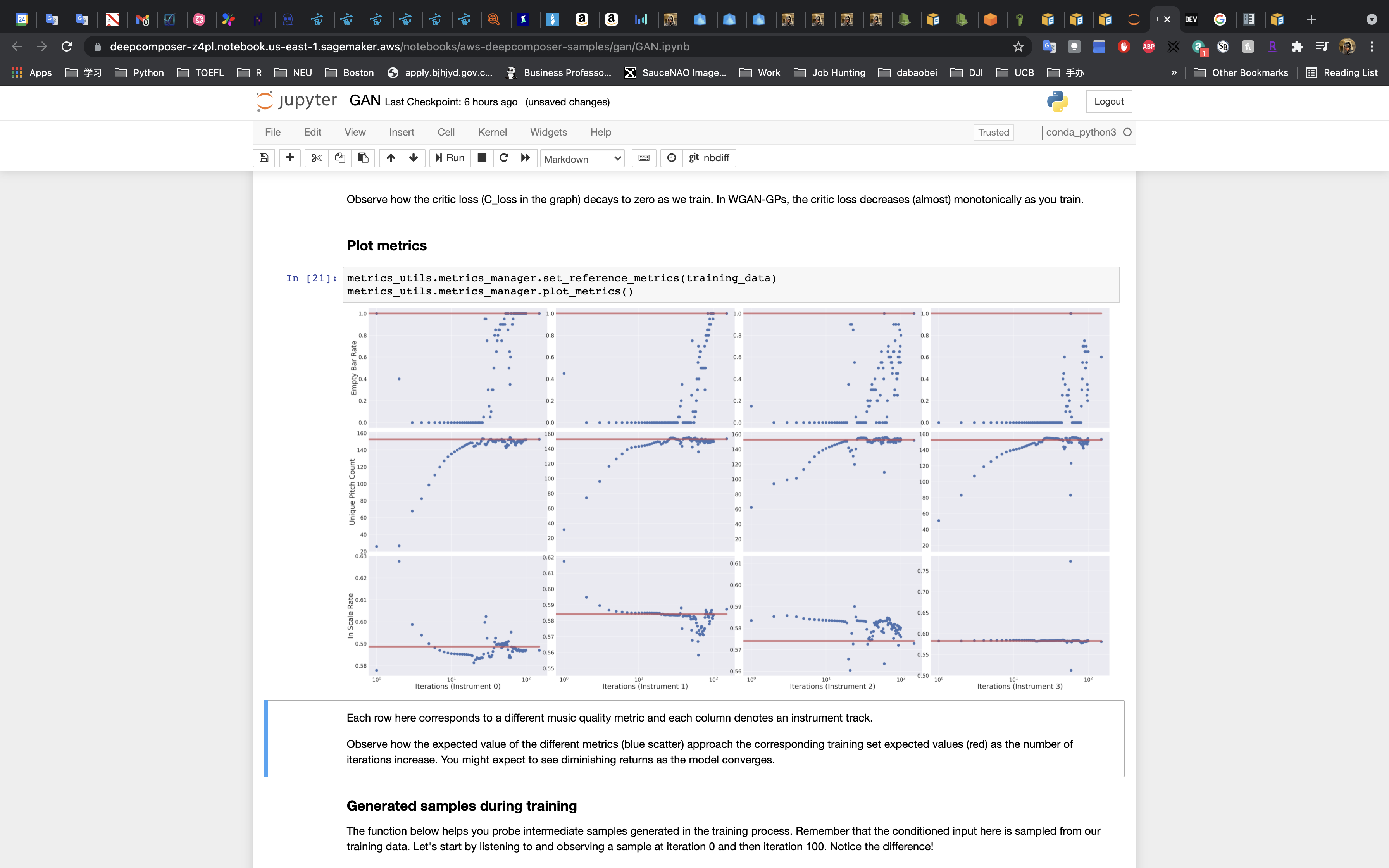
- Check to see if the losses for the networks are converging
- Look at commonly used musical metrics of the generated sample and compared them to the training dataset.
Evaluating Our Training Results
Run the cell to restore the saved checkpoint. If you don’t want to wait to complete the training you can use data from a pre-trained model by setting TRAIN = False in the cell.
- Run the cell to plot the losses.
- Run the cell to plot the metrics.
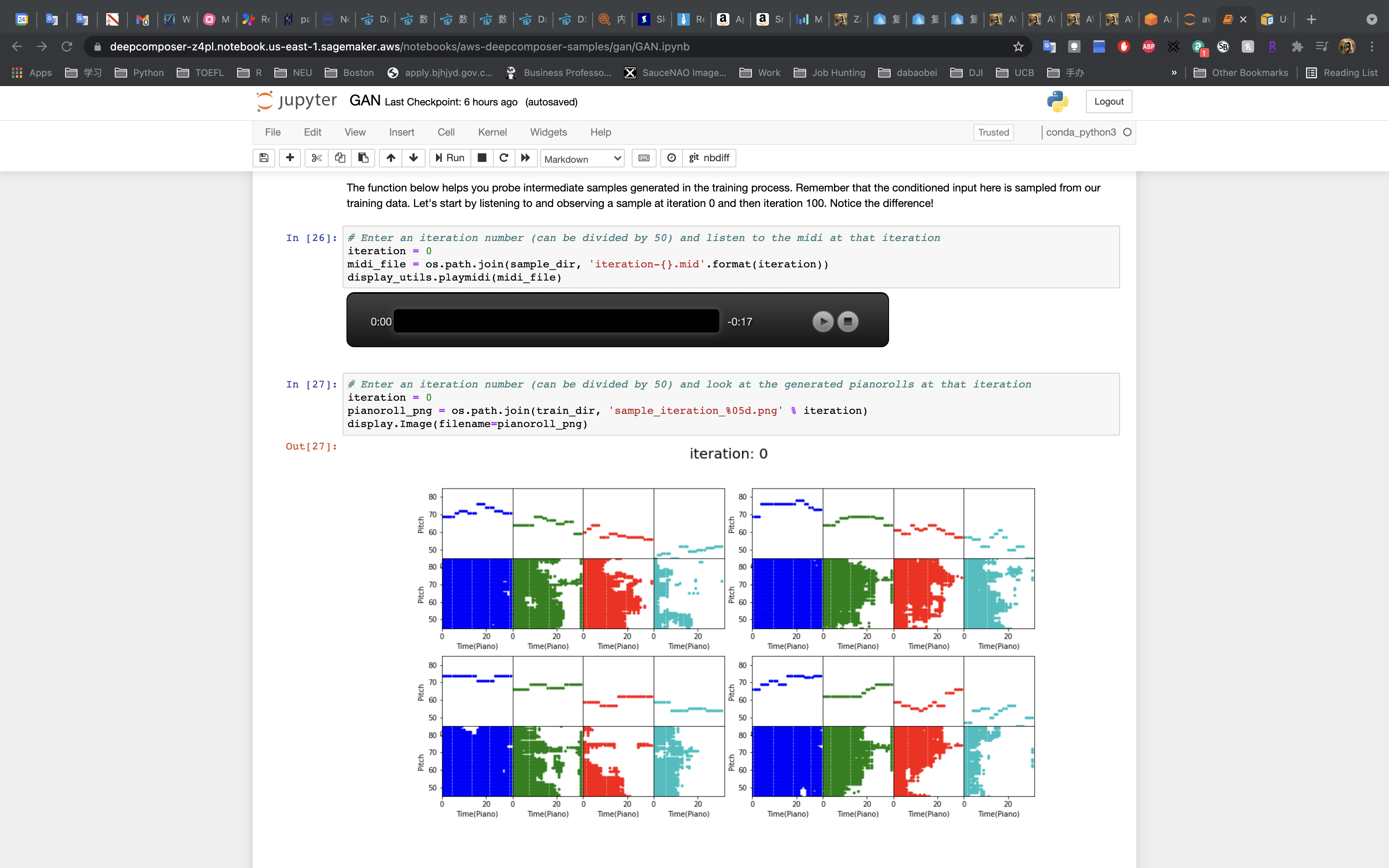
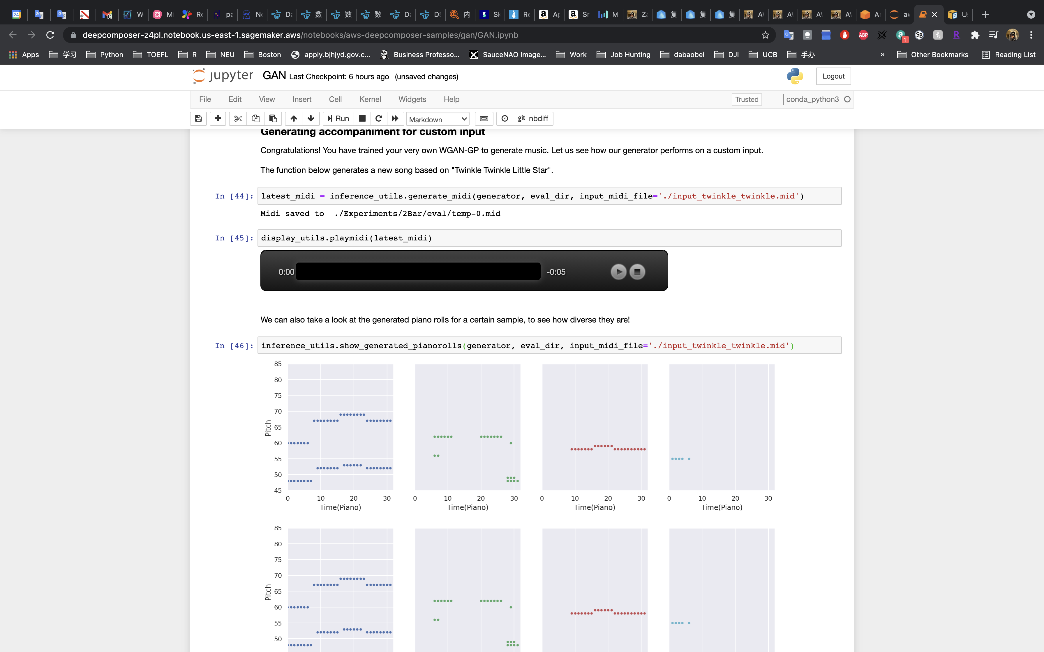
Evaluate the Generated Music
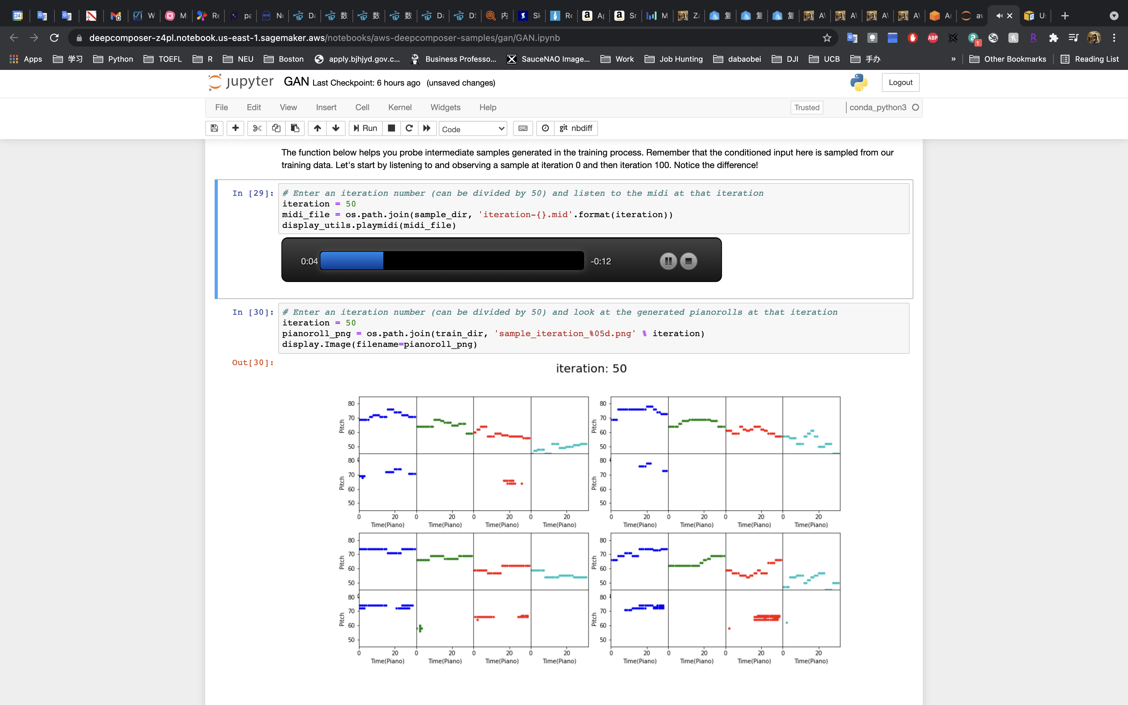
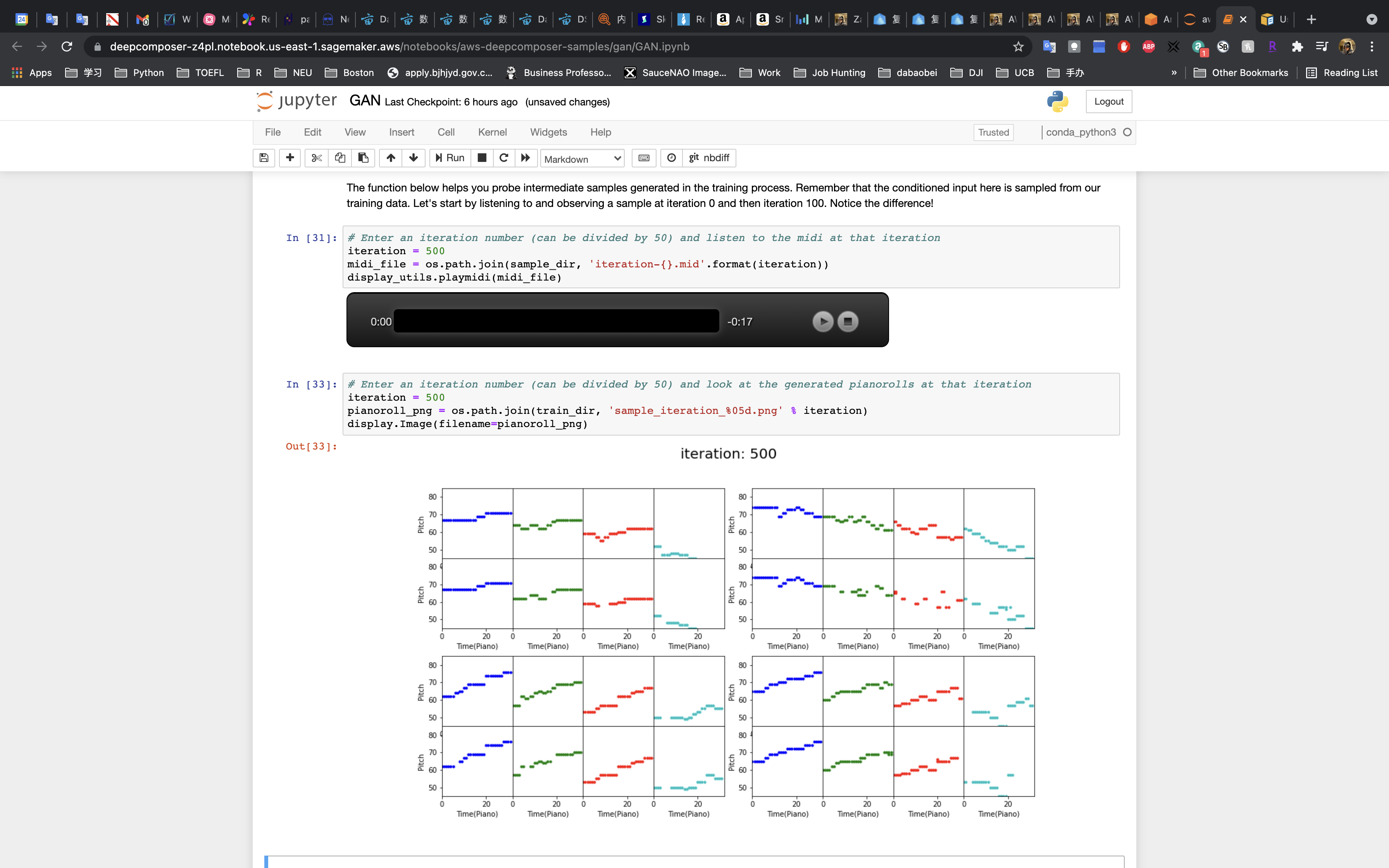
In the first cell, enter 0 as the iteration number.
run the cell and play the music snippet.
Or listen to this example snippet from iteration 0:
The iteration = 500 is much better than iteration = 50 and iteration = 0. The music is better and more consecutive.
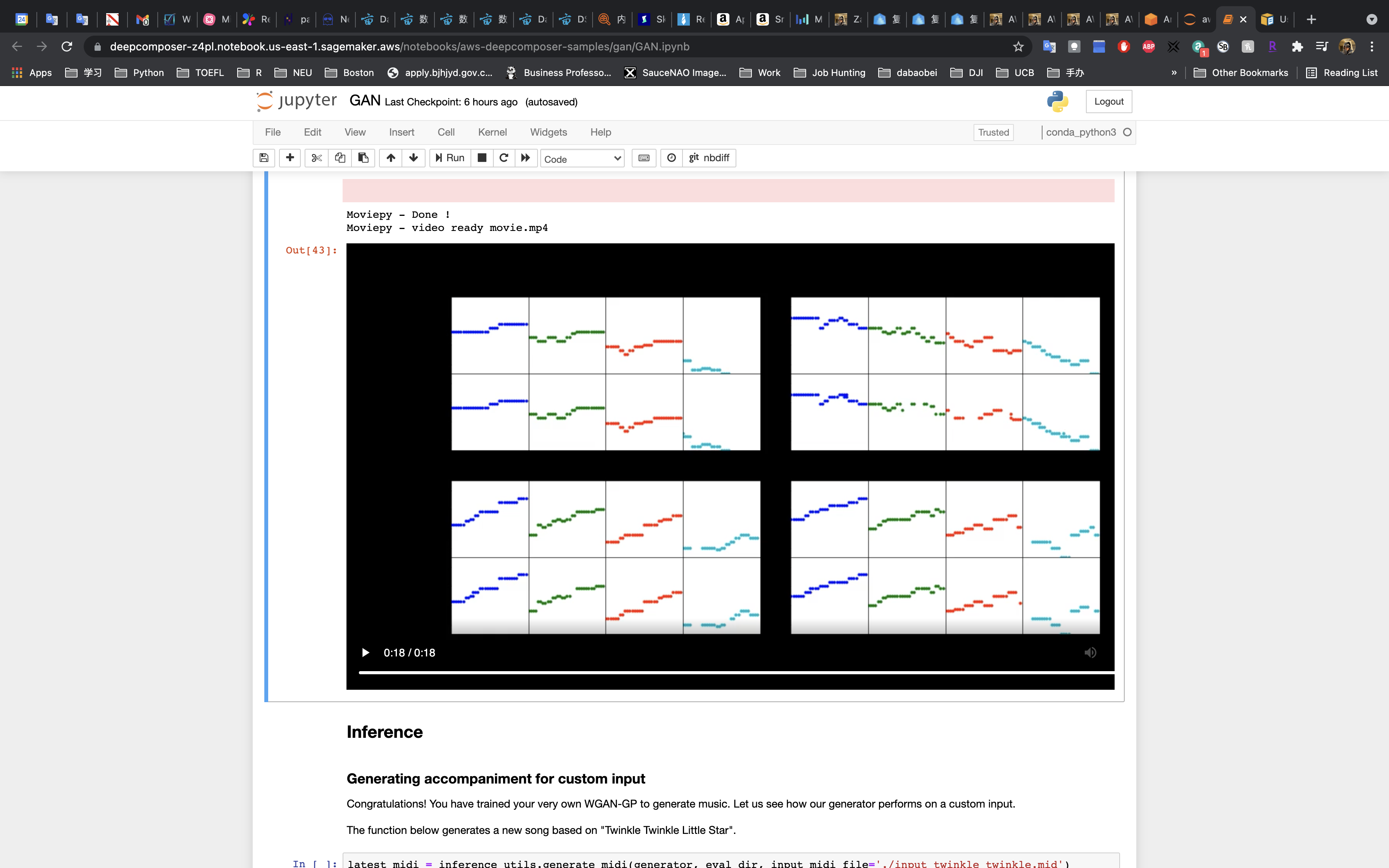
Watch the Evolution of the Model!
Run the next cell to create a video to see how the generated piano rolls change over time.
Inference
Now that the GAN has been trained we can run it on a custom input to generate music.
Run the cell to generate a new song based on “Twinkle Twinkle Little Star”.
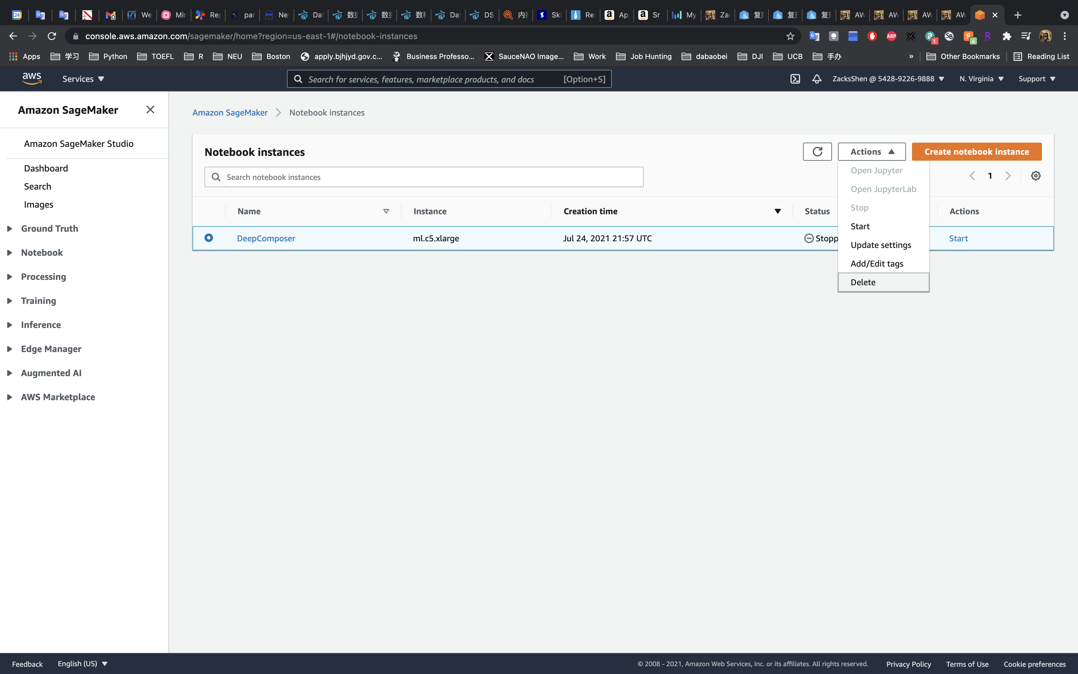
Stop and Delete the Jupyter Notebook
This project is not covered by the AWS Free Tier so your project will continue to accrue costs as long as it is running.
Select your notebook instance, then click on Actions -> Stop
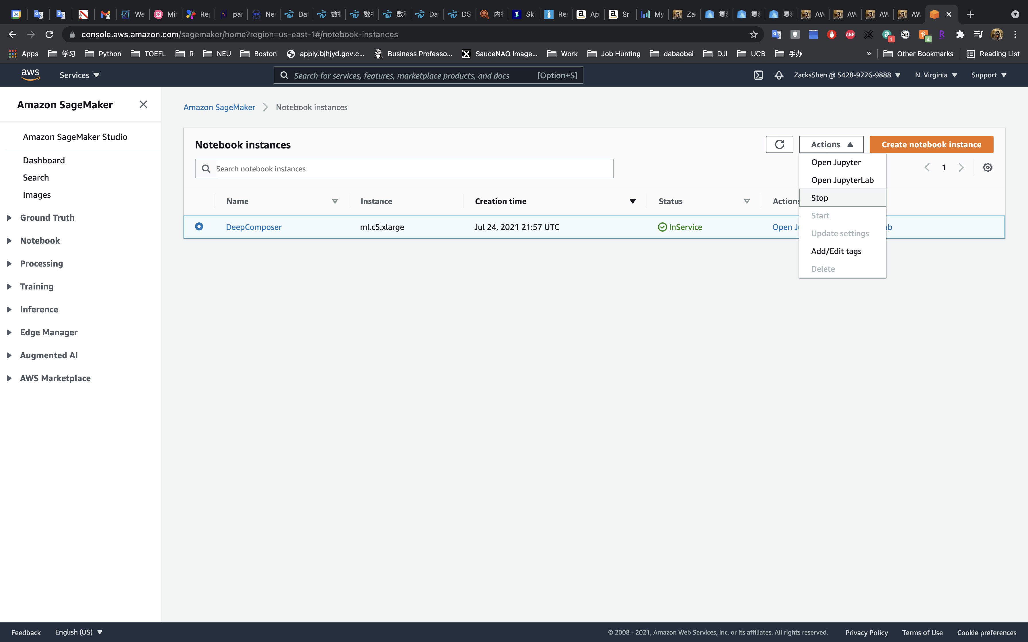
Wait until your instance shows Stopped.
Click on Actions -> Delete
Recap
In this demo we learned how to setup a Jupyter notebook in Amazon SageMaker, reviewed a machine learning code, and what data preparation, model training, and model evaluation can look like in a notebook instance. While this was a fun use case for us to explore, the concepts and techniques can be applied to other machine learning projects like an object detector or a sentiment analysis on text.