Data8

Data Science

DATA 8
What is Data Science?
The Best Python Libraries for Data Science and Machine Learning
Test statistics explained

---

What is Data Science?

What is Data Science?
Data Science is about drawing useful conclusions from large and diverse data sets through exploration, prediction, and inference.

• Exploration involves identifying patterns in information.
  • Primary tools for exploration are visualizations and descriptive statistics.
• Prediction involves using information we know to make informed guesses about values we wish we knew.
  • For prediction are machine learning and optimization
• Inference involves quantifying our degree of certainty: will the patterns that we found in our data also appear in new observations? How accurate are our predictions?
  • For inference are statistical tests and models.

Components

• Statistics is a central component of data science because statistics studies how to make robust conclusions based on incomplete information.
• Computing is a central component because programming allows us to apply analysis techniques to the large and diverse data sets that arise in real-world applications: not just numbers, but text, images, videos, and sensor readings.
• Data science is all of these things, but it is more than the sum of its parts because of the applications.

Through understanding a particular domain, data scientists learn to ask appropriate questions about their data and correctly interpret the answers provided by our inferential and computational tools.

---

Introduction

Data are descriptions of the world around us, collected through observation and stored on computers. Computers enable us to infer properties of the world from these descriptions. Data science is the discipline of drawing conclusions from data using computation. There are three core aspects of effective data analysis: exploration, prediction, and inference. This text develops a consistent approach to all three, introducing statistical ideas and fundamental ideas in computer science concurrently. We focus on a minimal set of core techniques that can be applied to a vast range of real-world applications. A foundation in data science requires not only understanding statistical and computational techniques, but also recognizing how they apply to real scenarios.

For whatever aspect of the world we wish to study—whether it’s the Earth’s weather, the world’s markets, political polls, or the human mind—data we collect typically offer an incomplete description of the subject at hand. A central challenge of data science is to make reliable conclusions using this partial information.

In this endeavor, we will combine two essential tools: computation and randomization. For example, we may want to understand climate change trends using temperature observations. Computers will allow us to use all available information to draw conclusions. Rather than focusing only on the average temperature of a region, we will consider the whole range of temperatures together to construct a more nuanced analysis. Randomness will allow us to consider the many different ways in which incomplete information might be completed. Rather than assuming that temperatures vary in a particular way, we will learn to use randomness as a way to imagine many possible scenarios that are all consistent with the data we observe.

Applying this approach requires learning to program a computer, and so this text interleaves a complete introduction to programming that assumes no prior knowledge. Readers with programming experience will find that we cover several topics in computation that do not appear in a typical introductory computer science curriculum. Data science also requires careful reasoning about numerical quantities, but this text does not assume any background in mathematics or statistics beyond basic algebra. You will find very few equations in this text. Instead, techniques are described to readers in the same language in which they are described to the computers that execute them—a programming language.

---

Computational Tools

This text uses the Python 3 programming language, along with a standard set of numerical and data visualization tools that are used widely in commercial applications, scientific experiments, and open-source projects. Python has recruited enthusiasts from many professions that use data to draw conclusions. By learning the Python language, you will join a million-person-strong community of software developers and data scientists.

Getting Started. The easiest and recommended way to start writing programs in Python is to log into the companion site for this text, datahub.berkeley.edu. If you have a @berkeley.edu email address, you already have full access to the programming environment hosted on that site. If not, please complete this form to request access.

You are not at all restricted to using this web-based programming environment. A Python program can be executed by any computer, regardless of its manufacturer or operating system, provided that support for the language is installed. If you wish to install the version of Python and its accompanying libraries that will match this text, we recommend the Anaconda distribution that packages together the Python 3 language interpreter, IPython libraries, and the Jupyter notebook environment.

This text includes a complete introduction to all of these computational tools. You will learn to write programs, generate images from data, and work with real-world data sets that are published online.

---

Statistical Techniques

The discipline of statistics has long addressed the same fundamental challenge as data science: how to draw robust conclusions about the world using incomplete information. One of the most important contributions of statistics is a consistent and precise vocabulary for describing the relationship between observations and conclusions. This text continues in the same tradition, focusing on a set of core inferential problems from statistics: testing hypotheses, estimating confidence, and predicting unknown quantities.

Data science extends the field of statistics by taking full advantage of computing, data visualization, machine learning, optimization, and access to information. The combination of fast computers and the Internet gives anyone the ability to access and analyze vast datasets: millions of news articles, full encyclopedias, databases for any domain, and massive repositories of music, photos, and video.

Applications to real data sets motivate the statistical techniques that we describe throughout the text. Real data often do not follow regular patterns or match standard equations. The interesting variation in real data can be lost by focusing too much attention on simplistic summaries such as average values. Computers enable a family of methods based on resampling that apply to a wide range of different inference problems, take into account all available information, and require few assumptions or conditions. Although these techniques have often been reserved for advanced courses in statistics, their flexibility and simplicity are a natural fit for data science applications.

---

Why Data Science?

Most important decisions are made with only partial information and uncertain outcomes. However, the degree of uncertainty for many decisions can be reduced sharply by access to large data sets and the computational tools required to analyze them effectively. Data-driven decision making has already transformed a tremendous breadth of industries, including finance, advertising, manufacturing, and real estate. At the same time, a wide range of academic disciplines are evolving rapidly to incorporate large-scale data analysis into their theory and practice.

Studying data science enables individuals to bring these techniques to bear on their work, their scientific endeavors, and their personal decisions. Critical thinking has long been a hallmark of a rigorous education, but critiques are often most effective when supported by data. A critical analysis of any aspect of the world, may it be business or social science, involves inductive reasoning; conclusions can rarely been proven outright, but only supported by the available evidence. Data science provides the means to make precise, reliable, and quantitative arguments about any set of observations. With unprecedented access to information and computing, critical thinking about any aspect of the world that can be measured would be incomplete without effective inferential techniques.

The world has too many unanswered questions and difficult challenges to leave this critical reasoning to only a few specialists. All educated members of society can build the capacity to reason about data. The tools, techniques, and data sets are all readily available; this text aims to make them accessible to everyone.

---

Plotting the classics

Program: Data8-1.3.ipynb

In this example, we will explore statistics for two classic novels: The Adventures of Huckleberry Finn by Mark Twain, and Little Women by Louisa May Alcott. The text of any book can be read by a computer at great speed. Books published before 1923 are currently in the public domain, meaning that everyone has the right to copy or use the text in any way. Project Gutenberg is a website that publishes public domain books online. Using Python, we can load the text of these books directly from the web.

This example is meant to illustrate some of the broad themes of this text. Don’t worry if the details of the program don’t yet make sense. Instead, focus on interpreting the images generated below. Later sections of the text will describe most of the features of the Python programming language used below.

First, we read the text of both books into lists of chapters, called huck_finn_chapters and little_women_chapters. In Python, a name cannot contain any spaces, and so we will often use an underscore _ to stand in for a space. The = in the lines below give a name on the left to the result of some computation described on the right. A uniform resource locator or URL is an address on the Internet for some content; in this case, the text of a book. The # symbol starts a comment, which is ignored by the computer but helpful for people reading the code.

Python

import urllib.request
import pandas as pd

# Read two books, fast!

# Define book url of The Adventures of Huckleberry Finn
huck_finn_url = 'https://www.inferentialthinking.com/data/huck_finn.txt'
# Read book
with urllib.request.urlopen(huck_finn_url) as response:
   html = response.read()
# Decode binary to string
huck_finn_text = html.decode('utf-8')
# Remove all '\r\n' in the original string
huck_finn_text = "".join(huck_finn_text.splitlines())
# Split the string in list according to keyword 'CHAPTER '], and only get the items after 44th
huck_finn_chapters = huck_finn_text.split('CHAPTER ')[44:]

# Define book url of Little Women*
little_women_url = 'https://www.inferentialthinking.com/data/little_women.txt'
# Read book
with urllib.request.urlopen(little_women_url) as response:
   html = response.read()
# Decode binary to string
little_women_text = html.decode('utf-8')
# Remove all '\r\n' in the original string
little_women_text = "".join(little_women_text.splitlines())
# Split the string in list according to keyword 'CHAPTER '], and only get the items after 1st
little_women_chapters = little_women_text.split('CHAPTER ')[1:]

While a computer cannot understand the text of a book, it can provide us with some insight into the structure of the text. The name huck_finn_chapters is currently bound to a list of all the chapters in the book. We can place them into a table to see how each chapter begins.

Python

import pandas as pd

# Display the chapters of Huckleberry Finn in a table.
pd.DataFrame(data=huck_finn_chapters, columns=['Chapters'])

	Chapters
0	I.YOU don't know about me without you have rea...
1	II.WE went tiptoeing along a path amongst the ...
2	III.WELL, I got a good going-over in the morni...
3	IV.WELL, three or four months run along, and i...
4	V.I had shut the door to.  Then I turned aroun...
...	...
38	XXXIX.IN the morning we went up to the village...
39	XL.WE was feeling pretty good after breakfast,...
40	XLI.THE doctor was an old man; a very nice, ki...
41	XLII.THE old man was uptown again before break...
42	THE LASTTHE first time I catched Tom private I...

43 rows × 1 columns

Each chapter begins with a chapter number in Roman numerals, followed by the first sentence of the chapter. Project Gutenberg has printed the first word of each chapter in upper case.

---

Literary Characters

The Adventures of Huckleberry Finn describes a journey that Huck and Jim take along the Mississippi River. Tom Sawyer joins them towards the end as the action heats up. Having loaded the text, we can quickly visualize how many times these characters have each been mentioned at any point in the book.

Python

import numpy as np
import plotly.express as px

# Get data from huck_finn_chapters
data = {
    'Jim': np.char.count(huck_finn_chapters, 'Jim'),
    'Tom': np.char.count(huck_finn_chapters, 'Tom'),
    'Huck': np.char.count(huck_finn_chapters, 'Huck')
}
# Define counts as a dataframe from data
counts = pd.DataFrame(data)
# Return cumulative sum over counts
cum_counts = counts.cumsum()
# Add a new attribute(column) Chapter
cum_counts['Chapter'] = np.arange(1, 44, 1)
cum_counts

	Jim	Tom	Huck	Chapter
0	0	6	3	1
1	16	30	5	2
2	16	35	7	3
3	24	35	8	4
4	24	35	8	5
...	...	...	...	...
38	345	177	69	39
39	358	188	72	40
40	358	196	72	41
41	370	226	74	42
42	376	232	78	43

43 rows × 4 columns

plotly.express.line

Python

# Plot the cumulative counts:
# how many times in Chapter 1, how many times in Chapters 1 and 2, and so on.

fig = px.line(cum_counts, x='Chapter', y=['Jim', 'Tom', 'Huck'], title='Cumulative Number of Times Each Name Appears')
fig.show()

In the plot above, the horizontal axis shows chapter numbers and the vertical axis shows how many times each character has been mentioned up to and including that chapter.

You can see that Jim is a central character by the large number of times his name appears. Notice how Tom is hardly mentioned for much of the book until he arrives and joins Huck and Jim, after Chapter 30. His curve and Jim’s rise sharply at that point, as the action involving both of them intensifies. As for Huck, his name hardly appears at all, because he is the narrator.

---

Little Women is a story of four sisters growing up together during the civil war. In this book, chapter numbers are spelled out and chapter titles are written in all capital letters.

Python

# The chapters of Little Women, in a table
pd.DataFrame(data=little_women_chapters, columns=['Chapters'])

	Chapters
0	ONEPLAYING PILGRIMS"Christmas won't be Christm...
1	TWOA MERRY CHRISTMASJo was the first to wake i...
2	THREETHE LAURENCE BOY"Jo! Jo! Where are you?...
3	FOURBURDENS"Oh, dear, how hard it does seem to...
4	FIVEBEING NEIGHBORLY"What in the world are you...
...	...
42	FORTY-THREESURPRISESJo was alone in the twilig...
43	FORTY-FOURMY LORD AND LADY"Please, Madam Mothe...
44	FORTY-FIVEDAISY AND DEMII cannot feel that I h...
45	FORTY-SIXUNDER THE UMBRELLAWhile Laurie and Am...
46	FORTY-SEVENHARVEST TIMEFor a year Jo and her P...

47 rows × 1 columns

We can track the mentions of main characters to learn about the plot of this book as well. The protagonist Jo interacts with her sisters Meg, Beth, and Amy regularly, up until Chapter 27 when she moves to New York alone.

Python

# Get data little_women_chapters
data = {
    'Amy': np.char.count(little_women_chapters, 'Amy'),
    'Beth': np.char.count(little_women_chapters, 'Beth'),
    'Jo': np.char.count(little_women_chapters, 'Jo'),
    'Meg': np.char.count(little_women_chapters, 'Meg'),
    'Laurie': np.char.count(little_women_chapters, 'Laurie')
}
# Define counts as a dataframe from data
counts = pd.DataFrame(data)
# Return cumulative sum over counts
cum_counts = counts.cumsum()
# Add a new attribute(column) Chapter
cum_counts['Chapter'] = np.arange(1, 48, 1)
cum_counts

	Amy	Beth	Jo	Meg	Laurie	Chapter
0	23	26	44	26	0	1
1	36	38	65	46	0	2
2	38	40	127	82	16	3
3	52	58	161	99	16	4
4	58	72	216	112	51	5
...	...	...	...	...	...	...
42	619	459	1435	673	571	43
43	632	459	1444	673	581	44
44	633	461	1450	675	581	45
45	635	462	1506	679	583	46
46	645	465	1543	685	596	47

47 rows × 6 columns

plotly.express.line

Python

# Plot the cumulative counts.

fig = px.line(cum_counts, x='Chapter', y=['Amy', 'Beth', 'Jo', 'Meg', 'Laurie'], title='Cumulative Number of Times Each Name Appears')
fig.show()

Laurie is a young man who marries one of the girls in the end. See if you can use the plots to guess which one.

---

Inspiration

See if we can use this tech to count the number of positive reviews and negative reviews on a company in a news for judging the influence of the breaking news on its stock price.

---

Another Kind of Character

In some situations, the relationships between quantities allow us to make predictions. This text will explore how to make accurate predictions based on incomplete information and develop methods for combining multiple sources of uncertain information to make decisions.

As an example of visualizing information derived from multiple sources, let us first use the computer to get some information that would be tedious to acquire by hand. In the context of novels, the word “character” has a second meaning: a printed symbol such as a letter or number or punctuation symbol. Here, we ask the computer to count the number of characters and the number of periods in each chapter of both Huckleberry Finn and Little Women.

Python

# In each chapter, count the number of all characters;
# call this the "length" of the chapter.
# Also count the number of periods.

chars_periods_huck_finn = pd.DataFrame({
        'Huck Finn Chapter Length': [len(s) for s in huck_finn_chapters],
        'Number of Periods': np.char.count(huck_finn_chapters, '.')})

chars_periods_little_women = pd.DataFrame({
        'Little Women Chapter Length': [len(s) for s in little_women_chapters],
        'Number of Periods': np.char.count(little_women_chapters, '.')})

Here are the data for Huckleberry Finn. Each row of the table corresponds to one chapter of the novel and displays the number of characters as well as the number of periods in the chapter. Not surprisingly, chapters with fewer characters also tend to have fewer periods, in general: the shorter the chapter, the fewer sentences there tend to be, and vice versa. The relation is not entirely predictable, however, as sentences are of varying lengths and can involve other punctuation such as question marks.

Python

chars_periods_huck_finn

	Huck Finn Chapter Length	Number of Periods
0	6970	66
1	11874	117
2	8460	72
3	6755	84
4	8095	91
...	...	...
38	10763	96
39	11386	60
40	13278	77
41	15565	92
42	21461	228

43 rows × 2 columns

Here are the corresponding data for Little Women.

Python

chars_periods_little_women

	Little Women Chapter Length	Number of Periods
0	21496	189
1	21941	188
2	20335	231
3	25213	195
4	23115	255
...	...	...
42	32811	305
43	10166	95
44	12390	96
45	27078	234
46	40592	392

47 rows × 2 columns

You can see that the chapters of Little Women are in general longer than those of Huckleberry Finn. Let us see if these two simple variables – the length and number of periods in each chapter – can tell us anything more about the two books. One way to do this is to plot both sets of data on the same axes.

In the plot below, there is a dot for each chapter in each book. Blue dots correspond to Huckleberry Finn and gold dots to Little Women. The horizontal axis represents the number of periods and the vertical axis represents the number of characters.

plotly.express.scatter

Python

import plotly.graph_objects as go

fig = go.Figure()

# Add traces
fig.add_trace(go.Scatter(x=chars_periods_huck_finn.loc[:, 'Number of Periods'],
                    y=chars_periods_huck_finn.loc[:, 'Huck Finn Chapter Length'],
                    mode='markers',
                    name='Huck Finn Chapter'))
fig.add_trace(go.Scatter(x=chars_periods_little_women.loc[:, 'Number of Periods'],
                    y=chars_periods_little_women.loc[:, 'Little Women Chapter Length'],
                    mode='markers',
                    name='Little Women'))
fig.update_layout(
    xaxis_title='Number of periods in chapter',
    yaxis_title='Number of characters in chapter',
    width=1200, height=800
    )
  
fig.show()

The plot shows us that many but not all of the chapters of Little Women are longer than those of Huckleberry Finn, as we had observed by just looking at the numbers. But it also shows us something more. Notice how the blue points are roughly clustered around a straight line, as are the yellow points. Moreover, it looks as though both colors of points might be clustered around the same straight line.

Now look at all the chapters that contain about 100 periods. The plot shows that those chapters contain about 10,000 characters to about 15,000 characters, roughly. That’s about 100 to 150 characters per period.

Indeed, it appears from looking at the plot that on average both books tend to have somewhere between 100 and 150 characters between periods, as a very rough estimate. Perhaps these two great 19th century novels were signaling something so very familiar to us now: the 140-character limit of Twitter.

---

Causality and Experiments

Causality and Experiments

---

Causality and Experiments

“These problems are, and will probably ever remain, among the inscrutable secrets of nature. They belong to a class of questions radically inaccessible to the human intelligence.” —The Times of London, September 1849, on how cholera is contracted and spread

Does the death penalty have a deterrent effect? Is chocolate good for you? What causes breast cancer?

All of these questions attempt to assign a cause to an effect. A careful examination of data can help shed light on questions like these. In this section you will learn some of the fundamental concepts involved in establishing causality.

Observation is a key to good science. An observational study is one in which scientists make conclusions based on data that they have observed but had no hand in generating. In data science, many such studies involve observations on a group of individuals, a factor of interest called a treatment, and an outcome measured on each individual.

It is easiest to think of the individuals as people. In a study of whether chocolate is good for the health, the individuals would indeed be people, the treatment would be eating chocolate, and the outcome might be a measure of heart disease. But individuals in observational studies need not be people. In a study of whether the death penalty has a deterrent effect, the individuals could be the 50 states of the union. A state law allowing the death penalty would be the treatment, and an outcome could be the state’s murder rate.

The fundamental question is whether the treatment has an effect on the outcome. Any relation between the treatment and the outcome is called an association. If the treatment causes the outcome to occur, then the association is causal. Causality is at the heart of all three questions posed at the start of this section. For example, one of the questions was whether chocolate directly causes improvements in health, not just whether there there is a relation between chocolate and health.

The establishment of causality often takes place in two stages. First, an association is observed. Next, a more careful analysis leads to a decision about causality.

---

Observation and Visualization: John Snow and the Broad Street Pump

One of the most powerful examples of astute observation eventually leading to the establishment of causality dates back more than 150 years. To get your mind into the right timeframe, try to imagine London in the 1850’s. It was the world’s wealthiest city but many of its people were desperately poor. Charles Dickens, then at the height of his fame, was writing about their plight. Disease was rife in the poorer parts of the city, and cholera was among the most feared. It was not yet known that germs cause disease; the leading theory was that “miasmas” were the main culprit. Miasmas manifested themselves as bad smells, and were thought to be invisible poisonous particles arising out of decaying matter. Parts of London did smell very bad, especially in hot weather. To protect themselves against infection, those who could afford to held sweet-smelling things to their noses.

For several years, a doctor by the name of John Snow had been following the devastating waves of cholera that hit England from time to time. The disease arrived suddenly and was almost immediately deadly: people died within a day or two of contracting it, hundreds could die in a week, and the total death toll in a single wave could reach tens of thousands. Snow was skeptical of the miasma theory. He had noticed that while entire households were wiped out by cholera, the people in neighboring houses sometimes remained completely unaffected. As they were breathing the same air—and miasmas—as their neighbors, there was no compelling association between bad smells and the incidence of cholera.

Snow had also noticed that the onset of the disease almost always involved vomiting and diarrhea. He therefore believed that the infection was carried by something people ate or drank, not by the air that they breathed. His prime suspect was water contaminated by sewage.

At the end of August 1854, cholera struck in the overcrowded Soho district of London. As the deaths mounted, Snow recorded them diligently, using a method that went on to become standard in the study of how diseases spread: he drew a map. On a street map of the district, he recorded the location of each death.

Here is Snow’s original map. Each black bar represents one death. When there are multiple deaths at the same address, the bars corresponding to those deaths are stacked on top of each other. The black discs mark the locations of water pumps. The map displays a striking revelation—the deaths are roughly clustered around the Broad Street pump.

Snow studied his map carefully and investigated the apparent anomalies. All of them implicated the Broad Street pump. For example:

• There were deaths in houses that were nearer the Rupert Street pump than the Broad Street pump. Though the Rupert Street pump was closer as the crow flies, it was less convenient to get to because of dead ends and the layout of the streets. The residents in those houses used the Broad Street pump instead.
• There were no deaths in two blocks just east of the pump. That was the location of the Lion Brewery, where the workers drank what they brewed. If they wanted water, the brewery had its own well.
• There were scattered deaths in houses several blocks away from the Broad Street pump. Those were children who drank from the Broad Street pump on their way to school. The pump’s water was known to be cool and refreshing.

The final piece of evidence in support of Snow’s theory was provided by two isolated deaths in the leafy and genteel Hampstead area, quite far from Soho. Snow was puzzled by these until he learned that the deceased were Mrs. Susannah Eley, who had once lived in Broad Street, and her niece. Mrs. Eley had water from the Broad Street pump delivered to her in Hampstead every day. She liked its taste.

Later it was discovered that a cesspit that was just a few feet away from the well of the Broad Street pump had been leaking into the well. Thus the pump’s water was contaminated by sewage from the houses of cholera victims.

Snow used his map to convince local authorities to remove the handle of the Broad Street pump. Though the cholera epidemic was already on the wane when he did so, it is possible that the disabling of the pump prevented many deaths from future waves of the disease.

The removal of the Broad Street pump handle has become the stuff of legend. At the Centers for Disease Control (CDC) in Atlanta, when scientists look for simple answers to questions about epidemics, they sometimes ask each other, “Where is the handle to this pump?”

Snow’s map is one of the earliest and most powerful uses of data visualization. Disease maps of various kinds are now a standard tool for tracking epidemics.

Towards Causality

Though the map gave Snow a strong indication that the cleanliness of the water supply was the key to controlling cholera, he was still a long way from a convincing scientific argument that contaminated water was causing the spread of the disease. To make a more compelling case, he had to use the method of comparison.

Scientists use comparison to identify an association between a treatment and an outcome. They compare the outcomes of a group of individuals who got the treatment (the treatment group) to the outcomes of a group who did not (the control group). For example, researchers today might compare the average murder rate in states that have the death penalty with the average murder rate in states that don’t.

If the results are different, that is evidence for an association. To determine causation, however, even more care is needed.

---

Snow’s “Grand Experiment”

Encouraged by what he had learned in Soho, Snow completed a more thorough analysis. For some time, he had been gathering data on cholera deaths in an area of London that was served by two water companies. The Lambeth water company drew its water upriver from where sewage was discharged into the River Thames. Its water was relatively clean. But the Southwark and Vauxhall (S&V) company drew its water below the sewage discharge, and thus its supply was contaminated.

The map below shows the areas served by the two companies. Snow honed in on the region where the two service areas overlap.

Snow noticed that there was no systematic difference between the people who were supplied by S&V and those supplied by Lambeth. “Each company supplies both rich and poor, both large houses and small; there is no difference either in the condition or occupation of the persons receiving the water of the different Companies … there is no difference whatever in the houses or the people receiving the supply of the two Water Companies, or in any of the physical conditions with which they are surrounded …”

The only difference was in the water supply, “one group being supplied with water containing the sewage of London, and amongst it, whatever might have come from the cholera patients, the other group having water quite free from impurity.”

Confident that he would be able to arrive at a clear conclusion, Snow summarized his data in the table below.

Supply Area	Number of houses	cholera deaths	deaths per 10,000 houses
S&V	40,046	1,263	315
Lambeth	26,107	98	37
Rest of London	256,423	1,422	59

The numbers pointed accusingly at S&V. The death rate from cholera in the S&V houses was almost ten times the rate in the houses supplied by Lambeth.

---

Establishing Causality

In the language developed earlier in the section, you can think of the people in the S&V houses as the treatment group, and those in the Lambeth houses at the control group. A crucial element in Snow’s analysis was that the people in the two groups were comparable to each other, apart from the treatment.

In order to establish whether it was the water supply that was causing cholera, Snow had to compare two groups that were similar to each other in all but one aspect—their water supply. Only then would he be able to ascribe the differences in their outcomes to the water supply. If the two groups had been different in some other way as well, it would have been difficult to point the finger at the water supply as the source of the disease. For example, if the treatment group consisted of factory workers and the control group did not, then differences between the outcomes in the two groups could have been due to the water supply, or to factory work, or both. The final picture would have been much more fuzzy.

Snow’s brilliance lay in identifying two groups that would make his comparison clear. He had set out to establish a causal relation between contaminated water and cholera infection, and to a great extent he succeeded, even though the miasmatists ignored and even ridiculed him. Of course, Snow did not understand the detailed mechanism by which humans contract cholera. That discovery was made in 1883, when the German scientist Robert Koch isolated the Vibrio cholerae, the bacterium that enters the human small intestine and causes cholera.

In fact the Vibrio cholerae had been identified in 1854 by Filippo Pacini in Italy, just about when Snow was analyzing his data in London. Because of the dominance of the miasmatists in Italy, Pacini’s discovery languished unknown. But by the end of the 1800’s, the miasma brigade was in retreat. Subsequent history has vindicated Pacini and John Snow. Snow’s methods led to the development of the field of epidemiology, which is the study of the spread of diseases.

Confounding

Let us now return to more modern times, armed with an important lesson that we have learned along the way:

In an observational study, if the treatment and control groups differ in ways other than the treatment, it is difficult to make conclusions about causality.

An underlying difference between the two groups (other than the treatment) is called a confounding factor, because it might confound you (that is, mess you up) when you try to reach a conclusion.

Example: Coffee and lung cancer. Studies in the 1960’s showed that coffee drinkers had higher rates of lung cancer than those who did not drink coffee. Because of this, some people identified coffee as a cause of lung cancer. But coffee does not cause lung cancer. The analysis contained a confounding factor—smoking. In those days, coffee drinkers were also likely to have been smokers, and smoking does cause lung cancer. Coffee drinking was associated with lung cancer, but it did not cause the disease.

Confounding factors are common in observational studies. Good studies take great care to reduce confounding and to account for its effects.

---

Randomization

An excellent way to avoid confounding is to assign individuals to the treatment and control groups at random, and then administer the treatment to those who were assigned to the treatment group. Randomization keeps the two groups similar apart from the treatment.

If you are able to randomize individuals into the treatment and control groups, you are running a randomized controlled experiment, also known as a randomized controlled trial (RCT). Sometimes, people’s responses in an experiment are influenced by their knowing which group they are in. So you might want to run a blind experiment in which individuals do not know whether they are in the treatment group or the control group. To make this work, you will have to give the control group a placebo, which is something that looks exactly like the treatment but in fact has no effect.

Randomized controlled experiments have long been a gold standard in the medical field, for example in establishing whether a new drug works. They are also becoming more commonly used in other fields such as economics.

Example: Welfare subsidies in Mexico. In Mexican villages in the 1990’s, children in poor families were often not enrolled in school. One of the reasons was that the older children could go to work and thus help support the family. Santiago Levy , a minister in Mexican Ministry of Finance, set out to investigate whether welfare programs could be used to increase school enrollment and improve health conditions. He conducted an RCT on a set of villages, selecting some of them at random to receive a new welfare program called PROGRESA. The program gave money to poor families if their children went to school regularly and the family used preventive health care. More money was given if the children were in secondary school than in primary school, to compensate for the children’s lost wages, and more money was given for girls attending school than for boys. The remaining villages did not get this treatment, and formed the control group. Because of the randomization, there were no confounding factors and it was possible to establish that PROGRESA increased school enrollment. For boys, the enrollment increased from 73% in the control group to 77% in the PROGRESA group. For girls, the increase was even greater, from 67% in the control group to almost 75% in the PROGRESA group. Due to the success of this experiment, the Mexican government supported the program under the new name OPORTUNIDADES, as an investment in a healthy and well educated population.

In some situations it might not be possible to carry out a randomized controlled experiment, even when the aim is to investigate causality. For example, suppose you want to study the effects of alcohol consumption during pregnancy, and you randomly assign some pregnant women to your “alcohol” group. You should not expect cooperation from them if you present them with a drink. In such situations you will almost invariably be conducting an observational study, not an experiment. Be alert for confounding factors.

---

Endnote

In the terminology that we have developed, John Snow conducted an observational study, not a randomized experiment. But he called his study a “grand experiment” because, as he wrote, “No fewer than three hundred thousand people … were divided into two groups without their choice, and in most cases, without their knowledge …”

Studies such as Snow’s are sometimes called “natural experiments.” However, true randomization does not simply mean that the treatment and control groups are selected “without their choice.”

The method of randomization can be as simple as tossing a coin. It may also be quite a bit more complex. But every method of randomization consists of a sequence of carefully defined steps that allow chances to be specified mathematically. This has two important consequences.

1. It allows us to account—mathematically—for the possibility that randomization produces treatment and control groups that are quite different from each other.
2. It allows us to make precise mathematical statements about differences between the treatment and control groups. This in turn helps us make justifiable conclusions about whether the treatment has any effect.

In this course, you will learn how to conduct and analyze your own randomized experiments. That will involve more detail than has been presented in this chapter. For now, just focus on the main idea: to try to establish causality, run a randomized controlled experiment if possible. If you are conducting an observational study, you might be able to establish association but it will be harder to establish causation. Be extremely careful about confounding factors before making conclusions about causality based on an observational study.

Terminology

• observational study
• treatment
• outcome
• association
• causal association
• causality
• comparison
• treatment group
• control group
• epidemiology
• confounding
• randomization
• randomized controlled experiment
• randomized controlled trial (RCT)
• blind
• placebo

Fun facts

1. John Snow is sometimes called the father of epidemiology, but he was an anesthesiologist by profession. One of his patients was Queen Victoria, who was an early recipient of anesthetics during childbirth.

2. Florence Nightingale, the originator of modern nursing practices and famous for her work in the Crimean War, was a die-hard miasmatist. She had no time for theories about contagion and germs, and was not one for mincing her words. “There is no end to the absurdities connected with this doctrine,” she said. “Suffice it to say that in the ordinary sense of the word, there is no proof such as would be admitted in any scientific enquiry that there is any such thing as contagion.”

3. A later RCT established that the conditions on which PROGRESA insisted—children going to school, preventive health care—were not necessary to achieve increased enrollment. Just the financial boost of the welfare payments was sufficient.

Good reads

The Strange Case of the Broad Street Pump: John Snow and the Mystery of Cholera by Sandra Hempel, published by our own University of California Press, reads like a whodunit. It was one of the main sources for this section’s account of John Snow and his work. A word of warning: some of the contents of the book are stomach-churning.

Poor Economics, the best seller by Abhijit Banerjee and Esther Duflo of MIT, is an accessible and lively account of ways to fight global poverty. It includes numerous examples of RCTs, including the PROGRESA example in this section.

---

Programming in Python

Programming in Python

---

Programming in Python

Programming can dramatically improve our ability to collect and analyze information about the world, which in turn can lead to discoveries through the kind of careful reasoning demonstrated in the previous section. In data science, the purpose of writing a program is to instruct a computer to carry out the steps of an analysis. Computers cannot study the world on their own. People must describe precisely what steps the computer should take in order to collect and analyze data, and those steps are expressed through programs.

---

Expressions

Programming languages are much simpler than human languages. Nonetheless, there are some rules of grammar to learn in any language, and that is where we will begin. In this text, we will use the Python programming language. Learning the grammar rules is essential, and the same rules used in the most basic programs are also central to more sophisticated programs.

Programs are made up of expressions, which describe to the computer how to combine pieces of data. For example, a multiplication expression consists of a * symbol between two numerical expressions. Expressions, such as 3 * 4, are evaluated by the computer. The value (the result of evaluation) of the last expression in each cell, 12 in this case, is displayed below the cell.

Python

3 * 4
# 12

The grammar rules of a programming language are rigid. In Python, the * symbol cannot appear twice in a row. The computer will not try to interpret an expression that differs from its prescribed expression structures. Instead, it will show a SyntaxError error. The Syntax of a language is its set of grammar rules, and a SyntaxError indicates that an expression structure doesn’t match any of the rules of the language.

Python

3 * * 4

'''
  File "<ipython-input-2-012ea60b41dd>", line 1
    3 * * 4
        ^
SyntaxError: invalid syntax
'''

Small changes to an expression can change its meaning entirely. Below, the space between the ‘s has been removed. Because ** appears between two numerical expressions, the expression is a well-formed exponentiation expression (the first number raised to the power of the second: 3 times 3 times 3 times 3). The symbols * and * are called operators, and the values they combine are called operands.

Python

3 ** 4
# 81

Common Operators. Data science often involves combining numerical values, and the set of operators in a programming language are designed to so that expressions can be used to express any sort of arithmetic. In Python, the following operators are essential. See more Python Operators

Expression Type	Operator	Example	Value
Addition	+	2 + 3	5
Subtraction	-	2 - 3	-1
Multiplication	*	2 * 3	6
Division	/	7 / 3	2.66667
Remainder	%	7 % 3	1
Exponentiation	**	2 ** 0.5	1.41421

Python expressions obey the same familiar rules of precedence as in algebra: multiplication and division occur before addition and subtraction. Parentheses can be used to group together smaller expressions within a larger expression.

Python

1 + 2 * 3 * 4 * 5 / 6 ** 3 + 7 + 8 - 9 + 10
# 17.555555555555557

Python

1 + 2 * (3 * 4 * 5 / 6) ** 3 + 7 + 8 - 9 + 10
# 2017.0

This chapter introduces many types of expressions. Learning to program involves trying out everything you learn in combination, investigating the behavior of the computer. What happens if you divide by zero? What happens if you divide twice in a row? You don’t always need to ask an expert (or the Internet); many of these details can be discovered by trying them out yourself.

---

Names

Names are given to values in Python using an assignment statement. In an assignment, a name is followed by =, which is followed by any expression. The value of the expression to the right of = is assigned to the name. Once a name has a value assigned to it, the value will be substituted for that name in future expressions.

Python

a = 10
b = 20
a + b
# 30

A previously assigned name can be used in the expression to the right of =.

Python

quarter = 1/4
half = 2 * quarter
half
# 0.5

However, only the current value of an expression is assigned to a name. If that value changes later, names that were defined in terms of that value will not change automatically.

Python

quarter = 4
half
# 0.5

Names must start with a letter, but can contain both letters and numbers. A name cannot contain a space; instead, it is common to use an underscore character _ to replace each space. Names are only as useful as you make them; it’s up to the programmer to choose names that are easy to interpret. Typically, more meaningful names can be invented than a and b. For example, to describe the sales tax on a $5 purchase in Berkeley, CA, the following names clarify the meaning of the various quantities involved.

Python

purchase_price = 5
state_tax_rate = 0.075
county_tax_rate = 0.02
city_tax_rate = 0
sales_tax_rate = state_tax_rate + county_tax_rate + city_tax_rate
sales_tax = purchase_price * sales_tax_rate
sales_tax
# 0.475

---

Example: Growth Rates

The relationship between two measurements of the same quantity taken at different times is often expressed as a growth rate. For example, the United States federal government employed 2,766,000 people in 2002 and 2,814,000 people in 2012. To compute a growth rate, we must first decide which value to treat as the initial amount. For values over time, the earlier value is a natural choice. Then, we divide the difference between the changed and initial amount by the initial amount.

Python

initial = 2766000
changed = 2814000
(changed - initial) / initial
# 0.01735357917570499

It is also typical to subtract one from the ratio of the two measurements, which yields the same value.

Python

(changed/initial) - 1
# 0.017353579175704903

This value is the growth rate over 10 years. A useful property of growth rates is that they don’t change even if the values are expressed in different units. So, for example, we can express the same relationship between thousands of people in 2002 and 2012.

Python

initial = 2766
changed = 2814
(changed/initial) - 1
# 0.017353579175704903

In 10 years, the number of employees of the US Federal Government has increased by only 1.74%. In that time, the total expenditures of the US Federal Government increased from $2.37 trillion to $3.38 trillion in 2012.

Python

initial = 2.37
changed = 3.38
(changed/initial) - 1
# 0.4261603375527425

A 42.6% increase in the federal budget is much larger than the 1.74% increase in federal employees. In fact, the number of federal employees has grown much more slowly than the population of the United States, which increased 9.21% in the same time period from 287.6 million people in 2002 to 314.1 million in 2012.

Python

initial = 287.6
changed = 314.1
(changed/initial) - 1
# 0.09214186369958277

A growth rate can be negative, representing a decrease in some value. For example, the number of manufacturing jobs in the US decreased from 15.3 million in 2002 to 11.9 million in 2012, a -22.2% growth rate.

Python

initial = 15.3
changed = 11.9
(changed/initial) - 1
# -0.2222222222222222

An annual growth rate is a growth rate of some quantity over a single year. An annual growth rate of 0.035, accumulated each year for 10 years, gives a much larger ten-year growth rate of 0.41 (or 41%).

Python

1.035 * 1.035 * 1.035 * 1.035 * 1.035 * 1.035 * 1.035 * 1.035 * 1.035 * 1.035 - 1
# 0.410598760621121

This same computation can be expressed using names and exponents.

Python

annual_growth_rate = 0.035
ten_year_growth_rate = (1 + annual_growth_rate) ** 10 - 1
ten_year_growth_rate
# 0.410598760621121

Likewise, a ten-year growth rate can be used to compute an equivalent annual growth rate. Below, t is the number of years that have passed between measurements. The following computes the annual growth rate of federal expenditures over the last 10 years.

Python

initial = 2.37
changed = 3.38
t = 10
(changed/initial) ** (1/t) - 1
# 0.03613617208346853

The total growth over 10 years is equivalent to a 3.6% increase each year.

In summary, a growth rate g is used to describe the relative size of an initial amount and a changed amount after some amount of time t. To compute changed , apply the growth rate g repeatedly, t times using exponentiation.

Python

initial * (1 + g) ** t

To compute g, raise the total growth to the power of 1/t and subtract one.

Python

(changed/initial) ** (1/t) - 1

---

Call Expressions

Call expressions invoke functions, which are named operations. The name of the function appears first, followed by expressions in parentheses.

Python

abs(-12)
# 12

Python

round(5 - 1.3)
# 4

Python

max(2, 2 + 3, 4)
# 5

In this last example, the max function is called on three arguments: 2, 5, and 4. The value of each expression within parentheses is passed to the function, and the function returns the final value of the full call expression. The max function can take any number of arguments and returns the maximum.

A few functions are available by default, such as abs and round, but most functions that are built into the Python language are stored in a collection of functions called a module. An import statement is used to provide access to a module, such as math or operator.

Python

import math
import operator
math.sqrt(operator.add(4, 5))
# 3.0

An equivalent expression could be expressed using the + and ** operators instead.

Python

(4 + 5) ** 0.5
# 3.0

Operators and call expressions can be used together in an expression. The percent difference between two values is used to compare values for which neither one is obviously initial or changed. For example, in 2014 Florida farms produced 2.72 billion eggs while Iowa farms produced 16.25 billion eggs (http://quickstats.nass.usda.gov/). The percent difference is 100 times the absolute value of the difference between the values, divided by their average. In this case, the difference is larger than the average, and so the percent difference is greater than 100.

Python

florida = 2.72
iowa = 16.25
100*abs(florida-iowa)/((florida+iowa)/2)
# 142.6462836056932

Learning how different functions behave is an important part of learning a programming language. A Jupyter notebook can assist in remembering the names and effects of different functions. When editing a code cell, press the tab key after typing the beginning of a name to bring up a list of ways to complete that name. For example, press tab after math. to see all of the functions available in the math module. Typing will narrow down the list of options. To learn more about a function, place a ? after its name. For example, typing math.log? will bring up a description of the log function in the math module.

Python

math.log?

'''
Docstring:
log(x, [base=math.e])
Return the logarithm of x to the given base.

If the base not specified, returns the natural logarithm (base e) of x.
Type:      builtin_function_or_method
'''

Return the logarithm of x to the given base.
If the base not specified, returns the natural logarithm (base e) of x.
The square brackets in the example call indicate that an argument is optional. That is, log can be called with either one or two arguments.

Python

math.log(16, 2)
# 4.0

Python

math.log(16)/math.log(2)
# 4.0

The list of Python’s built-in functions is quite long and includes many functions that are never needed in data science applications. The list of mathematical functions in the math module is similarly long. This text will introduce the most important functions in context, rather than expecting the reader to memorize or understand these lists.

---

Introduction to Tables

Program: Data8-3.4.ipynb

We can now apply Python to analyze data. We will work with data stored in Table structures.

Tables are a fundamental way of representing data sets. A table can be viewed in two ways:

• (NoSQL)a sequence of named columns that each describe a single attribute of all entries in a data set, or
• (SQL)a sequence of rows that each contain all information about a single individual in a data set.

We will study tables in great detail in the next several chapters. For now, we will just introduce a few methods without going into technical details.

The table cones has been imported for us; later we will see how, but here we will just work with it. First, let’s take a look at it.

Python

import pandas as pd

# Define cones' attributes
conesAttributes = ["Flavor", "Color", "Price"]

# Define cones' data, must be same sequence as attributes
conesData = [["strawberry", "pink", 3.55],
        ["chocolate", "light brown", 4.75],
        ["chocolate", "dark brown", 5.25],
        ["strawberry", "pink", 5.25],
        ["chocolate", "dark brown", 5.25],
        ["bubblegem", "pink", 4.75]]

# Define cones
cones = pd.DataFrame(data=conesData, columns=conesAttributes)

Python

# Show cones
cones

	Flavor	Color	Price
0	strawberry	pink	3.55
1	chocolate	light brown	4.75
2	chocolate	dark brown	5.25
3	strawberry	pink	5.25
4	chocolate	dark brown	5.25
5	bubblegem	pink	4.75

The table has six rows. Each row corresponds to one ice cream cone. The ice cream cones are the individuals.

Each cone has three attributes: flavor, color, and price. Each column contains the data on one of these attributes, and so all the entries of any single column are of the same kind. Each column has a label. We will refer to columns by their labels.

A table method is just like a function, but it must operate on a table. So the call looks like

name_of_table.method(arguments)

For example, if you want to see just the first two rows of a table, you can use the table method show.

Python

# Show first two rows
cones[:2]
# OR cones.iloc[:2]
# OR cones.iloc[0:2, :]

	Flavor	Color	Price
0	strawberry	pink	3.55
1	chocolate	light brown	4.75

… (4 rows omitted)

You can replace 2 by any number of rows. If you ask for more than six, you will only get six, because cones only has six rows.

---

Choosing Sets of Columns

The method loc creates a new table consisting of only the specified columns.

Python

# Show Flavor
cones.loc[:, ['Flavor']]

	Flavor
0	strawberry
1	chocolate
2	chocolate
3	strawberry
4	chocolate
5	bubblegem

This leaves the original table unchanged.

Python

# Show cones
cones

	Flavor	Color	Price
0	strawberry	pink	3.55
1	chocolate	light brown	4.75
2	chocolate	dark brown	5.25
3	strawberry	pink	5.25
4	chocolate	dark brown	5.25
5	bubblegem	pink	4.75

You can loc more than one column, by separating the column labels by commas.

Python

# Show Flavor, Price
cones.loc[:, ['Flavor', 'Price']]

	Flavor	Price
0	strawberry	3.55
1	chocolate	4.75
2	chocolate	5.25
3	strawberry	5.25
4	chocolate	5.25
5	bubblegem	4.75

You can also drop columns you don’t want. The table above can be created by dropping the Color column.

Python

# Drop Color
cones.drop(columns='Color')

	Flavor	Price
0	strawberry	3.55
1	chocolate	4.75
2	chocolate	5.25
3	strawberry	5.25
4	chocolate	5.25
5	bubblegem	4.75

You can name this new table and look at it again by just typing its name.

Python

# Redefine cones
cones = pd.DataFrame(data=conesData, columns=conesAttributes)

# Name a new dataframe without Color
no_colors = cones.drop(columns='Color')

# Show no_colors
no_colors

	Flavor	Price
0	strawberry	3.55
1	chocolate	4.75
2	chocolate	5.25
3	strawberry	5.25
4	chocolate	5.25
5	bubblegem	4.75

Like loc, the drop method creates a smaller table and leaves the original table unchanged. In order to explore your data, you can create any number of smaller tables by using choosing or dropping columns. It will do no harm to your original data table.

---

Sorting Rows

The sort method creates a new table by arranging the rows of the original table in ascending order of the values in the specified column. Here the cones table has been sorted in ascending order of the price of the cones.

Python

# Sort Price
cones.sort_values(by=["Price"])

	Flavor	Color	Price
0	strawberry	pink	3.55
1	chocolate	light brown	4.75
5	bubblegem	pink	4.75
2	chocolate	dark brown	5.25
3	strawberry	pink	5.25
4	chocolate	dark brown	5.25

To sort in descending order, you can use an optional argument to sort. As the name implies, optional arguments don’t have to be used, but they can be used if you want to change the default behavior of a method.

By default, sort sorts in increasing order of the values in the specified column. To sort in decreasing order, use the optional argument descending=True.

Python

# Sort Price Descending
cones.sort_values(by=["Price"], ascending=False)

	Flavor	Color	Price
2	chocolate	dark brown	5.25
3	strawberry	pink	5.25
4	chocolate	dark brown	5.25
1	chocolate	light brown	4.75
5	bubblegem	pink	4.75
0	strawberry	pink	3.55

Like loc, the drop method, the sort method leaves the original table unchanged.

---

Selecting Rows that Satisfy a Condition

The where method creates a new table consisting only of the rows that satisfy a given condition. In this section we will work with a very simple condition, which is that the value in a specified column must be equal to a value that we also specify. Thus the where method has two arguments.

The code in the cell below creates a table consisting only of the rows corresponding to chocolate cones.

Python

# Making boolean series for a cones
filter = cones['Flavor'] == "chocolate"

# Pass filter to cones
cones.where(filter, inplace=False)

	Flavor	Color	Price
0	NaN	NaN	NaN
1	chocolate	light brown	4.75
2	chocolate	dark brown	5.25
3	NaN	NaN	NaN
4	chocolate	dark brown	5.25
5	NaN	NaN	NaN

---

OR

Python

# Making boolean series for a cones
filter = cones['Flavor'] == "chocolate"

# Pass filter to cones
cones.loc[filter]

	Flavor	Color	Price
1	chocolate	light brown	4.75
2	chocolate	dark brown	5.25
4	chocolate	dark brown	5.25

---

The arguments, separated by a comma, are the label of the column and the value we are looking for in that column. The where method can also be used when the condition that the rows must satisfy is more complicated. In those situations the call will be a little more complicated as well.

It is important to provide the value exactly. For example, if we specify Chocolate instead of chocolate, then where correctly finds no rows where the flavor is Chocolate.

Python

# Making boolean series for a cones
filter = cones['Flavor'] == "chocolate"

# Pass filter to cones
cones.loc[filter]

	Flavor	Color	Price

---

Python

# Making boolean series for a cones
filter = cones['Flavor'] == "chocolate"

# Pass filter to cones
cones.where(filter, inplace=False)

	Flavor	Color	Price
0	NaN	NaN	NaN
1	NaN	NaN	NaN
2	NaN	NaN	NaN
3	NaN	NaN	NaN
4	NaN	NaN	NaN
5	NaN	NaN	NaN

Like all the other table methods in this section, where leaves the original table unchanged.

---

Example: Salaries in the NBA

“The NBA is the highest paying professional sports league in the world,” reported CNN in March 2016. The table nba contains the salaries of all National Basketball Association players in 2015-2016.

Each row represents one player. The columns are:

Column Label	Description
PLAYER	Player's name
POSITION	Player's position on team
TEAM	Team name
SALARY	Player's salary in 2015-2016, in millions of dollars

The code for the positions is PG (Point Guard), SG (Shooting Guard), PF (Power Forward), SF (Small Forward), and C (Center). But what follows doesn’t involve details about how basketball is played.

The first row shows that Paul Millsap, Power Forward for the Atlanta Hawks, had a salary of almost $18.7 million in 2015-2016.

Python

import pandas as pd

# Read nba csv
nba = pd.read_csv('https://raw.githubusercontent.com/ZacksAmber/Code/master/Data%20Science/Data8/Data%20Sets/nba.csv')

# Show nba
nba

	RANK	PLAYER	POSITION	TEAM	SALARY ($M)
0	1	Kobe Bryant	SF	Los Angeles Lakers	25.000000
1	2	Joe Johnson	SF	Brooklyn Nets	24.894863
2	3	LeBron James	SF	Cleveland Cavaliers	22.970500
3	4	Carmelo Anthony	SF	New York Knicks	22.875000
4	5	Dwight Howard	C	Houston Rockets	22.359364
...	...	...	...	...	...
412	413	Elliot Williams	SG	Memphis Grizzlies	0.055722
413	414	Phil Pressey	PG	Phoenix Suns	0.055722
414	415	Jordan McRae	SG	Phoenix Suns	0.049709
415	416	Cory Jefferson	PF	Phoenix Suns	0.049709
416	417	Thanasis Antetokounmpo	SF	New York Knicks	0.030888

417 rows × 5 columns

By default, the first 20 lines of a table are displayed. You can use head to display table more or fewer from the first row. To display the entire table, set pd.set_option("display.max_rows", None), then call the table directly.

Python

# Get default max_rows to show 
pd.get_option("max_rows")
# Set max_rows to unlimited
pd.set_option("display.max_rows", None)
# Set max_rows to 10
pd.set_option("max_rows", 10)
# Reset max_rows
pd.reset_option("max_rows")

Python

nba

---

Fans of Stephen Curry can find his row by using loc.

Python

# Filter "Stephen Curry"
filter = nba["PLAYER"] == "Stephen Curry"
nba.loc[filter]

	RANK	PLAYER	POSITION	TEAM	SALARY ($M)
56	57	Stephen Curry	PG	Golden State Warriors	11.370786

---

We can also create a new table called warriors consisting of just the data for the Golden State Warriors.

Python

# Filter "Golden State Warriors"
filter = nba["TEAM"] == "Golden State Warriors"
warriors = nba.loc[filter]
warriors

	RANK	PLAYER	POSITION	TEAM	SALARY ($M)
27	28	Klay Thompson	SG	Golden State Warriors	15.501000
33	34	Draymond Green	PF	Golden State Warriors	14.260870
37	38	Andrew Bogut	C	Golden State Warriors	13.800000
55	56	Andre Iguodala	SF	Golden State Warriors	11.710456
56	57	Stephen Curry	PG	Golden State Warriors	11.370786
100	101	Jason Thompson	PF	Golden State Warriors	7.008475
127	128	Shaun Livingston	PG	Golden State Warriors	5.543725
177	178	Harrison Barnes	SF	Golden State Warriors	3.873398
178	179	Marreese Speights	C	Golden State Warriors	3.815000
236	237	Leandro Barbosa	SG	Golden State Warriors	2.500000
267	268	Festus Ezeli	C	Golden State Warriors	2.008748
312	313	Brandon Rush	SF	Golden State Warriors	1.270964
335	336	Kevon Looney	SF	Golden State Warriors	1.131960
402	403	Anderson Varejao	PF	Golden State Warriors	0.289755

---

The nba table is sorted in alphabetical order of the team names. To see how the players were paid in 2015-2016, it is useful to sort the data by salary. Remember that by default, the sorting is in increasing order.

Python

# Sort nba based on SALARY, ascending=True
nba.sort_values(by=["SALARY ($M)"], ascending=True)

	RANK	PLAYER	POSITION	TEAM	SALARY ($M)
416	417	Thanasis Antetokounmpo	SF	New York Knicks	0.030888
415	416	Cory Jefferson	PF	Phoenix Suns	0.049709
414	415	Jordan McRae	SG	Phoenix Suns	0.049709
411	412	Orlando Johnson	SG	Phoenix Suns	0.055722
413	414	Phil Pressey	PG	Phoenix Suns	0.055722
...	...	...	...	...	...
4	5	Dwight Howard	C	Houston Rockets	22.359364
3	4	Carmelo Anthony	SF	New York Knicks	22.875000
2	3	LeBron James	SF	Cleveland Cavaliers	22.970500
1	2	Joe Johnson	SF	Brooklyn Nets	24.894863
0	1	Kobe Bryant	SF	Los Angeles Lakers	25.000000

417 rows × 5 columns

---

These figures are somewhat difficult to compare as some of these players changed teams during the season and received salaries from more than one team; only the salary from the last team appears in the table.

The CNN report is about the other end of the salary scale – the players who are among the highest paid in the world. To identify these players we can sort in descending order of salary and look at the top few rows.

Python

# Sort nba based on SALARY, ascending=False
nba.sort_values(by=["SALARY ($M)"], ascending=False)

	RANK	PLAYER	POSITION	TEAM	SALARY ($M)
0	1	Kobe Bryant	SF	Los Angeles Lakers	25.000000
1	2	Joe Johnson	SF	Brooklyn Nets	24.894863
2	3	LeBron James	SF	Cleveland Cavaliers	22.970500
3	4	Carmelo Anthony	SF	New York Knicks	22.875000
4	5	Dwight Howard	C	Houston Rockets	22.359364
...	...	...	...	...	...
412	413	Elliot Williams	SG	Memphis Grizzlies	0.055722
413	414	Phil Pressey	PG	Phoenix Suns	0.055722
414	415	Jordan McRae	SG	Phoenix Suns	0.049709
415	416	Cory Jefferson	PF	Phoenix Suns	0.049709
416	417	Thanasis Antetokounmpo	SF	New York Knicks	0.030888

417 rows × 5 columns

Kobe Bryant, since retired, was the highest earning NBA player in 2015-2016.

R.I.P Kobe.

---

Data Types

Data Types
Python Data Types

---

Every value has a type, and the built-in type function returns the type of the result of any expression.

One type we have encountered already is a built-in function. Python indicates that the type is a builtin_function_or_method; the distinction between a function and a method is not important at this stage.

Python

type(abs)
# builtin_function_or_method

This chapter will explore many useful types of data.

---

Numbers

Computers are designed to perform numerical calculations, but there are some important details about working with numbers that every programmer working with quantitative data should know. Python (and most other programming languages) distinguishes between two different types of numbers:

• Integers are called int values in the Python language. They can only represent whole numbers (negative, zero, or positive) that don’t have a fractional component.
• Real numbers are called float values (or floating point values) in the Python language. They can represent whole or fractional numbers but have some limitations.

The type of a number is evident from the way it is displayed: int values have no decimal point and float values always have a decimal point.

Python

# Some int values
2
# 2

Python

1 + 3
# 4

Python

-1234567890000000000
# -1234567890000000000

Python

# Some float values
1.2
# 1.2

Python

3.0
# 3.0

When a float value is combined with an int value using some arithmetic operator, then the result is always a float value. In most cases, two integers combine to form another integer, but any number (int or float) divided by another will be a float value. Very large or very small float values are displayed using scientific notation.

Python

1.5 + 2
# 3.5

Python

3 / 1
# 3.0

Python

-12345678900000000000.0
# -1.23456789e+19

The type function can be used to find the type of any number.

Python

type(3)
# int

Python

type(3 / 1)
# float

The type of an expression is the type of its final value. So, the type function will never indicate that the type of an expression is a name, because names are always evaluated to their assigned values.

Python

x = 3
type(x) # The type of x is an int, not a name
# int

Python

type(x + 2.5)
# float

---

More About Float Values

Float values are very flexible, but they do have limits.

1. A float can represent extremely large and extremely small numbers. There are limits, but you will rarely encounter them.
2. A float only represents 15 or 16 significant digits for any number; the remaining precision is lost. This limited precision is enough for the vast majority of applications.
3. After combining float values with arithmetic, the last few digits may be incorrect. Small rounding errors are often confusing when first encountered.

The first limit can be observed in two ways. If the result of a computation is a very large number, then it is represented as infinite. If the result is a very small number, then it is represented as zero.

Python

2e306 * 10
# 2e+307

Python

2e306 * 100
# inf

Python

2e-322 / 10
# 2e-323

Python

2e-322 / 100
# 0.0

The second limit can be observed by an expression that involves numbers with more than 15 significant digits. These extra digits are discarded before any arithmetic is carried out.

Python

0.6666666666666666 - 0.6666666666666666123456789
# 0.0

The third limit can be observed when taking the difference between two expressions that should be equivalent. For example, the expression 2 ** 0.5 computes the square root of 2, but squaring this value does not exactly recover 2.

Python

2 ** 0.5
# 1.4142135623730951

Python

(2 ** 0.5) * (2 ** 0.5)
# 2.0000000000000004

Python

(2 ** 0.5) * (2 ** 0.5) - 2
# 4.440892098500626e-16

The final result above is 0.0000000000000004440892098500626, a number that is very close to zero. The correct answer to this arithmetic expression is 0, but a small error in the final significant digit appears very different in scientific notation. This behavior appears in almost all programming languages because it is the result of the standard way that arithmetic is carried out on computers.

Although float values are not always exact, they are certainly reliable and work the same way across all different kinds of computers and programming languages.

---

Strings

Much of the world’s data is text, and a piece of text represented in a computer is called a string. A string can represent a word, a sentence, or even the contents of every book in a library. Since text can include numbers (like this: 5) or truth values (True), a string can also describe those things.

The meaning of an expression depends both upon its structure and the types of values that are being combined. So, for instance, adding two strings together produces another string. This expression is still an addition expression, but it is combining a different type of value.

Python

"data" + "science"
# 'datascience'

Addition is completely literal; it combines these two strings together without regard for their contents. It doesn’t add a space because these are different words; that’s up to the programmer (you) to specify.

Python

"data" + " " + "science"
# 'data science'

Single and double quotes can both be used to create strings: 'hi' and "hi" are identical expressions. Double quotes are often preferred because they allow you to include apostrophes inside of strings.

Python

"This won't work with a single-quoted string!"
# "This won't work with a single-quoted string!"

Why not? Try it out.

The str function returns a string representation of any value. Using this function, strings can be constructed that have embedded values.

Python

"That's " + str(1 + 1) + ' ' + str(True)
# "That's 2 True"

---

String Methods

From an existing string, related strings can be constructed using string methods, which are functions that operate on strings. These methods are called by placing a dot after the string, then calling the function.

For example, the following method generates an uppercased version of a string.

Python

"loud".upper()
# 'LOUD'

Perhaps the most important method is replace, which replaces all instances of a substring within the string. The replace method takes two arguments, the text to be replaced and its replacement.

Python

'hitchhiker'.replace('hi', 'ma')
# 'matchmaker'

String methods can also be invoked using variable names, as long as those names are bound to strings. So, for instance, the following two-step process generates the word “degrade” starting from “train” by first creating “ingrain” and then applying a second replacement.

Python

s = "train"
t = s.replace('t', 'ing')
u = t.replace('in', 'de')
u

# 'degrade'

Note that the line t = s.replace(‘t’, ‘ing’) doesn’t change the string s, which is still “train”. The method call s.replace(‘t’, ‘ing’) just has a value, which is the string “ingrain”.

Python

s
# 'train'

This is the first time we’ve seen methods, but methods are not unique to strings. As we will see shortly, other types of objects can have them.

---

Comparisons

Python Comparison Operators

Boolean values most often arise from comparison operators. Python includes a variety of operators that compare values. For example, 3 is larger than 1 + 1.

Python

3 > 1 + 1
# True

The value True indicates that the comparison is valid; Python has confirmed this simple fact about the relationship between 3 and 1+1. The full set of common comparison operators are listed below.

Comparison	Operator	True example	False Example
Less than	<	2 < 3	2 < 2
Greater than	>	3>2	3>3
Less than or equal	<=	2 <= 2	3 <= 2
Greater or equal	>=	3 >= 3	2 >= 3
Equal	==	3 == 3	3 == 2
Not equal	!=	3 != 2	2 != 2

An expression can contain multiple comparisons, and they all must hold in order for the whole expression to be True. For example, we can express that 1+1 is between 1 and 3 using the following expression.

Python

1 < 1 + 1 < 3
# True

The average of two numbers is always between the smaller number and the larger number. We express this relationship for the numbers x and y below. You can try different values of x and y to confirm this relationship.

Python

x = 12
y = 5
min(x, y) <= (x+y)/2 <= max(x, y)

# True

Strings can also be compared, and their order is alphabetical. A shorter string is less than a longer string that begins with the shorter string.

Python

"Dog" > "Catastrophe" > "Cat"
# True

---

Sequences

Sequences

---

Sequences

Values can be grouped together into collections, which allows programmers to organize those values and refer to all of them with a single name. By grouping values together, we can write code that performs a computation on many pieces of data at once.

Calling the function np.array on several values places them into an array, which is a kind of sequential collection. Below, we collect four different temperatures into an array called highs. These are the estimated average daily high temperatures over all land on Earth (in degrees Celsius) for the decades surrounding 1850, 1900, 1950, and 2000, respectively, expressed as deviations from the average absolute high temperature between 1951 and 1980, which was 14.48 degrees.

Python

import numpy as np

baseline_high = 14.48
highs = np.array([baseline_high - 0.880, baseline_high - 0.093,
                   baseline_high + 0.105, baseline_high + 0.684])
highs
# array([13.6  ,  14.387,  14.585,  15.164])

Collections allow us to pass multiple values into a function using a single name. For instance, the sum function computes the sum of all values in a collection, and the len function computes its length. (That’s the number of values we put in it.) Using them together, we can compute the average of a collection.

Python

sum(highs)/len(highs)
# 14.434000000000001

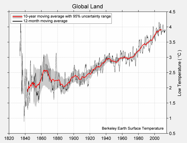
The complete chart of daily high and low temperatures appears below.

---

Mean of Daily High Temperature

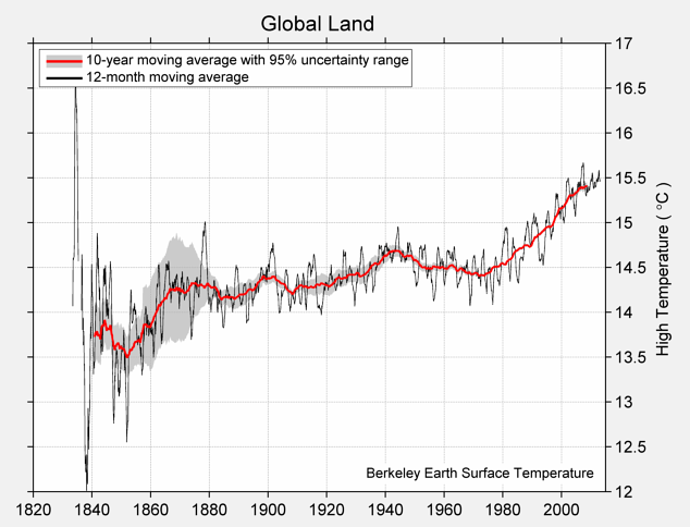
Mean of Daily Low Temperature

---

Arrays

While there are many kinds of collections in Python, we will work primarily with arrays in this class. We’ve already seen that the np.array function can be used to create arrays of numbers.

Arrays can also contain strings or other types of values, but a single array can only contain a single kind of data. (It usually doesn’t make sense to group together unlike data anyway.) For example:

Python

import numpy as np

english_parts_of_speech = np.array(["noun", "pronoun", "verb", "adverb", "adjective", "conjunction", "preposition", "interjection"])
english_parts_of_speech
# array(['noun', 'pronoun', 'verb', 'adverb', 'adjective', 'conjunction', 'preposition', 'interjection'], dtype='<U12')

Returning to the temperature data, we create arrays of average daily high temperatures for the decades surrounding 1850, 1900, 1950, and 2000.

Python

baseline_high = 14.48
highs = np.array([baseline_high - 0.880, 
                   baseline_high - 0.093,
                   baseline_high + 0.105, 
                   baseline_high + 0.684])
highs
# array([13.6  , 14.387, 14.585, 15.164])

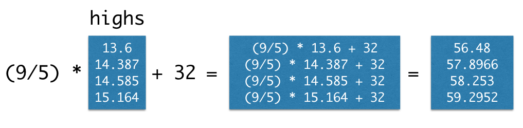
Arrays can be used in arithmetic expressions to compute over their contents. When an array is combined with a single number, that number is combined with each element of the array. Therefore, we can convert all of these temperatures to Fahrenheit by writing the familiar conversion formula.

Python

(9/5) * highs + 32
# array([56.48  , 57.8966, 58.253 , 59.2952])

Arrays also have methods, which are functions that operate on the array values. The mean of a collection of numbers is its average value: the sum divided by the length. Each pair of parentheses in the examples below is part of a call expression; it’s calling a function with no arguments to perform a computation on the array called highs.

Python

highs.size
# 4

Python

highs.sum()
# 57.736000000000004

Python

highs.mean()
# 14.434000000000001

---

Functions on Arrays

The numpy package, abbreviated np in programs, provides Python programmers with convenient and powerful functions for creating and manipulating arrays

Python

import numpy as np

For example, the diff function computes the difference between each adjacent pair of elements in an array. The first element of the diff is the second element minus the first.

Python

np.diff(highs)
# array([0.787, 0.198, 0.579])

Python

np.diff(np.array([4, 3, 2, 1]))
# array([1, 1, 1])

The full Numpy reference lists these functions exhaustively, but only a small subset are used commonly for data processing applications. These are grouped into different packages within np. Learning this vocabulary is an important part of learning the Python language, so refer back to this list often as you work through examples and problems.

However, you don’t need to memorize these. Use this as a reference.

Each of these functions takes an array as an argument and returns a single value.

Function	Description
np.prod	Multiply all elements together
np.sum	Add all elements together
np.all	Test whether all elements are true values (non-zero numbers are true)
np.any	Test whether any elements are true values (non-zero numbers are true)
np.count_nonzero	Count the number of non-zero elements

Each of these functions takes an array as an argument and returns an array of values.

Function	Description
np.diff	Difference between adjacent elements
np.round	Round each number to the nearest integer (whole number)
np.cumprod	A cumulative product: for each element, multiply all elements so far
np.cumsum	A cumulative sum: for each element, add all elements so far
np.exp	Exponentiate each element
np.log	Take the natural logarithm of each element
np.sqrt	Take the square root of each element
np.sort	Sort the elements

Each of these functions takes an array of strings and returns an array.

Function	Description
np.char.lower	Lowercase each element
np.char.upper	Uppercase each element
np.char.strip	Remove spaces at the beginning or end of each element
np.char.isalpha	Whether each element is only letters (no numbers or symbols)
np.char.isnumeric	Whether each element is only numeric (no letters)

Each of these functions takes both an array of strings and a search string; each returns an array.

Function	Description
np.char.count	Count the number of times a search string appears among the elements of an array
np.char.find	The position within each element that a search string is found first
np.char.rfind	The position within each element that a search string is found last
np.char.startswith	Whether each element starts with the search string

---

Ranges

A range is an array of numbers in increasing or decreasing order, each separated by a regular interval. Ranges are useful in a surprisingly large number of situations, so it’s worthwhile to learn about them.

Ranges are defined using the np.arange function, which takes either one, two, or three arguments: a start, and stop, and a step.

If you pass one argument to np.arange, this becomes the stop value, with start=0, step=1 assumed. Two arguments give the start and stop with step=1 assumed. Three arguments give the start, stop and step explicitly.

A range always includes its start value, but does not include its end value. It counts up by step, and it stops before it gets to the end.

np.arange(stop): An array starting with 0 of increasing consecutive integers, stopping before stop.

Python

import numpy as np

np.arange(5)
# array([0, 1, 2, 3, 4])

Notice how the array starts at 0 and goes only up to 4, not to the end value of 5.

---

np.arange(start=0, stop): An array of consecutive increasing integers from start, stopping before stop.

• The following two examples are the same.

Python

np.arange(3, 9)
# array([3, 4, 5, 6, 7, 8])

np.arange(start=3, stop=9)
# array([3, 4, 5, 6, 7, 8])

---

np.arange(start=0, stop, step=1): A range with a difference of step between each pair of consecutive values, starting from start and stopping before end.

• The following two examples are the same.

Python

np.arange(3, 30, 5)
# array([ 3,  8, 13, 18, 23, 28])

np.arange(start=3, stop=30, step=5)
# array([ 3,  8, 13, 18, 23, 28])

This array starts at 3, then takes a step of 5 to get to 8, then another step of 5 to get to 13, and so on.

When you specify a step, the start, end, and step can all be either positive or negative and may be whole numbers or fractions.

• The following two examples are the same.

Python

np.arange(1.5, -2, -0.5)
# array([ 1.5,  1. ,  0.5,  0. , -0.5, -1. , -1.5])

np.arange(start=1.5, stop=-2, step=-0.5)
# array([ 1.5,  1. ,  0.5,  0. , -0.5, -1. , -1.5])

---

Example: Leibniz’s formula for $\pi$

The great German mathematician and philosopher Gottfried Wilhelm Leibniz (1646 - 1716) discovered a wonderful formula for $\pi$ as an infinite sum of simple fractions. The formula is

$$\pi = 4 \cdot \left(1 - \frac{1}{3} + \frac{1}{5} - \frac{1}{7} + \frac{1}{9} - \frac{1}{11} + \dots\right)$$

Though some math is needed to establish this, we can use arrays to convince ourselves that the formula works. Let’s calculate the first 5000 terms of Leibniz’s infinite sum and see if it is close to $\pi$.

$$4 \cdot \left(1 - \frac{1}{3} + \frac{1}{5} - \frac{1}{7} + \frac{1}{9} - \frac{1}{11} + \dots - \frac{1}{9999} \right)$$

We will calculate this finite sum by adding all the positive terms first and then subtracting the sum of all the negative terms^[1] :

$$4 \cdot \left( \left(1 + \frac{1}{5} + \frac{1}{9} + \dots + \frac{1}{9997} \right) - \left(\frac{1}{3} + \frac{1}{7} + \frac{1}{11} + \dots + \frac{1}{9999} \right) \right)$$

The positive terms in the sum have 1, 5, 9, and so on in the denominators. The array by_four_to_20 contains these numbers up to 17:

Python

by_four_to_20 = np.arange(1, 20, 4)
by_four_to_20
# array([ 1,  5,  9, 13, 17])

To get an accurate approximation to $\pi$, we’ll use the much longer array positive_term_denominators.

Python

positive_term_denominators = np.arange(1, 10000, 4)
positive_term_denominators
# array([   1,    5,    9, ..., 9989, 9993, 9997])

The positive terms we actually want to add together are just 1 over these denominators:

Python

positive_terms = 1 / positive_term_denominators

The negative terms have 3, 7, 11, and so on on in their denominators. This array is just 2 added to positive_term_denominators.

Python

negative_terms = 1 / (positive_term_denominators + 2)

The overall sum is

Python

4 * ( sum(positive_terms) - sum(negative_terms) )
# 3.1413926535917955

This is very close to $\pi=3.14159…$. Leibniz’s formula is looking good!

---

More on Arrays

It’s often necessary to compute something that involves data from more than one array. If two arrays are of the same size, Python makes it easy to do calculations involving both arrays.

For our first example, we return once more to the temperature data. This time, we create arrays of average daily high and low temperatures for the decades surrounding 1850, 1900, 1950, and 2000.

Python

import numpy as np

baseline_high = 14.48
highs = np.array([
      baseline_high - 0.880, 
      baseline_high - 0.093,
      baseline_high + 0.105, 
      baseline_high + 0.684
])
highs
# array([ 13.6  ,  14.387,  14.585,  15.164])

Python

baseline_low = 3.00
lows = np.array([
      baseline_low - 0.872,
      baseline_low - 0.629,
      baseline_low - 0.126,
      baseline_low + 0.728
])
lows
# array([ 2.128,  2.371,  2.874,  3.728])

Suppose we’d like to compute the average daily range of temperatures for each decade. That is, we want to subtract the average daily high in the 1850s from the average daily low in the 1850s, and the same for each other decade.

We could write this laboriously using .item:

Python

np.array([
    highs.item(0) - lows.item(0),
    highs.item(1) - lows.item(1),
    highs.item(2) - lows.item(2),
    highs.item(3) - lows.item(3)
])
# array([11.472, 12.016, 11.711, 11.436])

As when we converted an array of temperatures from Celsius to Fahrenheit, Python provides a much cleaner way to write this:

Python

highs - lows
# array([11.472, 12.016, 11.711, 11.436])

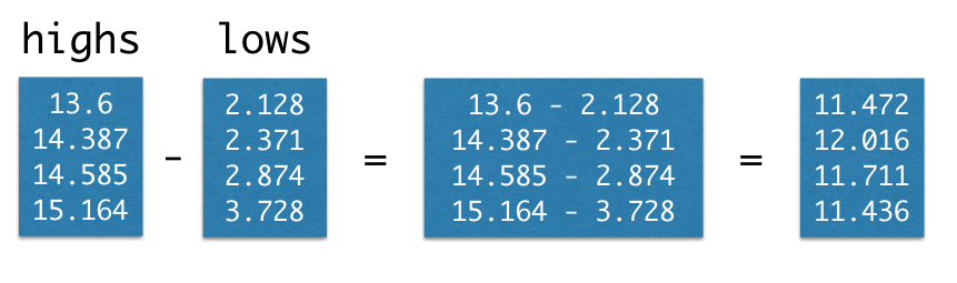
What we’ve seen in these examples are special cases of a general feature of arrays.

---

Elementwise arithmetic on pairs of numerical arrays

If an arithmetic operator acts on two arrays of the same size, then the operation is performed on each corresponding pair of elements in the two arrays. The final result is an array.

For example, if array1 and array2 have the same number of elements, then the value of array1 * array2 is an array. Its first element is the first element of array1 times the first element of array2, its second element is the second element of array1 times the second element of array2, and so on.

---

Example: Wallis’ Formula for $\pi$

The number $\pi$ is important in many different areas of math. Centuries before computers were invented, mathematicians worked on finding simple ways to approximate the numerical value of $\pi$. We have already seen Leibniz’s formula for $\pi$. About half a century before Leibniz, the English mathematician John Wallis (1616-1703) also expressed $\pi$ in terms of simple fractions, as an infinite product.

$$\pi = 2 \cdot \left( \frac{2}{1}\cdot\frac{2}{3}\cdot\frac{4}{3}\cdot\frac{4}{5}\cdot\frac{6}{5}\cdot\frac{6}{7}\dots \right)$$

This is a product of “even/odd” fractions. Let’s use arrays to multiply a million of them, and see if the product is close to $\pi$.

Remember that multiplication can done in any order^[2], so we can readjust our calculation to:

$$\pi \approx 2 \cdot \left( \frac{2}{1} \cdot \frac{4}{3} \cdot \frac{6}{5} \cdots \frac{1,000,000}{999999} \right) \cdot \left( \frac{2}{3} \cdot \frac{4}{5} \cdot \frac{6}{7} \cdots \frac{1,000,000}{1,000,001} \right)$$

We’re now ready to do the calculation. We start by creating an array of even numbers 2, 4, 6, and so on upto 1,000,000. Then we create two lists of odd numbers: 1, 3, 5, 7, … upto 999,999, and 3, 5, 7, … upto 1,000,001.

Python

even = np.arange(2, 1000001, 2)
one_below_even = even - 1
one_above_even = even + 1

Remember that np.prod multiplies all the elements of an array together. Now we can calculate Wallis’ product, to a good approximation.

Python

2 * np.prod(even/one_below_even) * np.prod(even/one_above_even)
# 3.1415910827951143

That’s $\pi$ correct to five decimal places. Wallis clearly came up with a great formula.

---

Tables

Tables
Program: Data8-6.ipynb

---

Tables

Code

Tables are a fundamental object type for representing data sets. A table can be viewed in two ways:

• a sequence of named columns that each describe a single aspect of all entries in a data set, or
• a sequence of rows that each contain all information about a single entry in a data set.
  In order to use tables, import all of the module called datascience, a module created for this text.

Python

import pandas as pd
import numpy as np

Empty tables can be created using the pd.DataFrame function. An empty table is usefuly because it can be extended to contain new rows and columns.

Python

pd.DataFrame()

The pd.DataFrame method on a table constructs a new table with additional labeled columns. Each column of a table is an array. To add one new column to a table, call df[] with a label and an array.

Below, we begin each example with an empty table that has no columns.

• Treat data keyword as row in a table.

Python

pd.DataFrame(columns=['Number of petals'], data=np.array([8, 34, 5]))

	Number of petals
0	8
1	34
2	5

To add two (or more) new columns, provide the label and array for each column in dict. All columns must have the same length, or an error will occur.

Python

pd.DataFrame({'Number of petals': np.array([8, 34, 5]),
              'Name': np.array(['lotus', 'sunflower', 'rose'])})

	Number of petals	Name
0	8	lotus
1	34	sunflower
2	5	rose

We can give this table a name, and then extend the table with another column. To add one new column to a table, call df[] with a label and an array.

Python

flowers = pd.DataFrame({'Number of petals': np.array([8, 34, 5]),
                        'Name': np.array(['lotus', 'sunflower', 'rose'])})
flowers['Color'] = np.array(['pink', 'yellow', 'red'])
flowers

	Number of petals	Name	Color
0	8	lotus	pink
1	34	sunflower	yellow
2	5	rose	red

---

Creating tables in this way involves a lot of typing. If the data have already been entered somewhere, it is usually possible to use Python to read it into a table, instead of typing it all in cell by cell.

Often, tables are created from files that contain comma-separated values. Such files are called CSV files.

Below, we use the pd method read_table to read a CSV file that contains some of the data used by Minard in his graphic about Napoleon’s Russian campaign. The data are placed in a table named minard.

pandas.read_csv

Python

# Read CSV
minard_cities = pd.read_csv('https://vincentarelbundock.github.io/Rdatasets/csv/HistData/Minard.cities.csv')
minard_temp = pd.read_csv('https://vincentarelbundock.github.io/Rdatasets/csv/HistData/Minard.temp.csv')
minard_troops = pd.read_csv('https://vincentarelbundock.github.io/Rdatasets/csv/HistData/Minard.troops.csv')

# Remove the 1st column which is rank
minard_cities = minard_cities.iloc[:, 1:]
minard_temp = minard_temp.iloc[:, 1:]
minard_troops = minard_troops.iloc[:, 1:]

Join the table minard_troops and minard_cities based on keys long and lat.

pandas.DataFrame.join

Python

# Join minard_troops and minard_cities
minard = minard_troops.join(minard_cities.set_index(['long', 'lat']), on=['long', 'lat'])
minard.head(20)

	long	lat	survivors	direction	group	city
0	24.0	54.9	340000	A	1	NaN
1	24.5	55.0	340000	A	1	NaN
2	25.5	54.5	340000	A	1	NaN
3	26.0	54.7	320000	A	1	NaN
4	27.0	54.8	300000	A	1	NaN
5	28.0	54.9	280000	A	1	NaN
6	28.5	55.0	240000	A	1	NaN
7	29.0	55.1	210000	A	1	NaN
8	30.0	55.2	180000	A	1	NaN
9	30.3	55.3	175000	A	1	NaN
10	32.0	54.8	145000	A	1	Smolensk
11	33.2	54.9	140000	A	1	Dorogobouge
12	34.4	55.5	127100	A	1	Chjat
13	35.5	55.4	100000	A	1	NaN
14	36.0	55.5	100000	A	1	Mojaisk
15	37.6	55.8	100000	A	1	Moscou
16	37.7	55.7	100000	R	1	NaN
17	37.5	55.7	98000	R	1	NaN
18	37.0	55.0	97000	R	1	NaN
19	36.8	55.0	96000	R	1	NaN

---

Filter the null data in column city.

pandas.DataFrame.isnull
pandas.DataFrame.notna
pandas.DataFrame.notnull

Python

# Filter the NaN(Null) value in city column
filter = minard['city'].notnull()
minard = minard[filter]
minard

	long	lat	survivors	direction	group	city
10	32.0	54.8	145000	A	1	Smolensk
11	33.2	54.9	140000	A	1	Dorogobouge
12	34.4	55.5	127100	A	1	Chjat
14	36.0	55.5	100000	A	1	Mojaisk
15	37.6	55.8	100000	A	1	Moscou
21	34.3	55.2	55000	R	1	Wixma
29	26.8	54.3	12000	R	1	Moiodexno
30	26.4	54.4	14000	R	1	Smorgoni
40	28.7	55.5	33000	A	2	Polotzk
41	28.7	55.5	33000	R	2	Polotzk

We will use this small table to demonstrate some useful Pandas.DataFrame methods. We will then use those same methods, and develop other methods, on much larger tables of data.

---

The Columns(Attributes) of the Table

pandas.DataFrame.columns

The method columns can be used to list the labels of all the columns. With minard we don’t gain much by this, but it can be very useful for tables that are so large that not all columns are visible on the screen.

Python

# The columns of the Table
minard.columns
# Index(['long', 'lat', 'survivors', 'direction', 'group', 'city'], dtype='object')

We can change column name using the rename method. This creates a new table and leaves minard unchanged.

pandas.DataFrame.rename

Python

# Rename column 'city' to 'city name', inplace=False
minard.rename(columns={'city': 'city name'})

	long	lat	survivors	direction	group	city name
10	32.0	54.8	145000	A	1	Smolensk
11	33.2	54.9	140000	A	1	Dorogobouge
12	34.4	55.5	127100	A	1	Chjat
14	36.0	55.5	100000	A	1	Mojaisk
15	37.6	55.8	100000	A	1	Moscou
21	34.3	55.2	55000	R	1	Wixma
29	26.8	54.3	12000	R	1	Moiodexno
30	26.4	54.4	14000	R	1	Smorgoni
40	28.7	55.5	33000	A	2	Polotzk
41	28.7	55.5	33000	R	2	Polotzk

Python

minard

	long	lat	survivors	direction	group	city
10	32.0	54.8	145000	A	1	Smolensk
11	33.2	54.9	140000	A	1	Dorogobouge
12	34.4	55.5	127100	A	1	Chjat
14	36.0	55.5	100000	A	1	Mojaisk
15	37.6	55.8	100000	A	1	Moscou
21	34.3	55.2	55000	R	1	Wixma
29	26.8	54.3	12000	R	1	Moiodexno
30	26.4	54.4	14000	R	1	Smorgoni
40	28.7	55.5	33000	A	2	Polotzk
41	28.7	55.5	33000	R	2	Polotzk

A common pattern is to assign the original name minard to the new table, so that all future uses of minard will refer to the relabeled table. Also, you can pass the inplace=True to rename method.

• inplace is a default False parameter of rename method

Python

# Rename column 'city' to 'city name', inplace=True
minard.rename(columns={'city': 'city name'}, inplace=True)
minard

	long	lat	survivors	direction	group	city name
10	32.0	54.8	145000	A	1	Smolensk
11	33.2	54.9	140000	A	1	Dorogobouge
12	34.4	55.5	127100	A	1	Chjat
14	36.0	55.5	100000	A	1	Mojaisk
15	37.6	55.8	100000	A	1	Moscou
21	34.3	55.2	55000	R	1	Wixma
29	26.8	54.3	12000	R	1	Moiodexno
30	26.4	54.4	14000	R	1	Smorgoni
40	28.7	55.5	33000	A	2	Polotzk
41	28.7	55.5	33000	R	2	Polotzk

OR

Python

# Rename column 'city' to 'city name'
# minard.rename(columns={'city name': 'city'}, inplace=True)
minard = minard.rename(columns={'city': 'city name'})

---

The Size of the Table

The method len(df.columns) gives the number of columns in the table, and len(df) gives the number of rows.

Python

# The number of columns in the table
len(minard.columns)
# 6

Python

# The number of rows in the table
len(minard)
# 10

---

Accessing the Data in a Column

pandas.DataFrame.iloc

We can use a column’s label to access the array of data in the column.

Python

minard['survivors']

'''
10    145000
11    140000
12    127100
14    100000
15    100000
21     55000
29     12000
30     14000
40     33000
41     33000
Name: survivors, dtype: int64
'''

You can also:

Python

minard.survivors


'''
10    145000
11    140000
12    127100
14    100000
15    100000
21     55000
29     12000
30     14000
40     33000
41     33000
Name: survivors, dtype: int64
'''

The 6 columns are indexed 0, 1, 2, 3, 4, and 5. The column survivors can also be accessed by using its column index.

Python

minard.iloc[:, 2]

'''
10    145000
11    140000
12    127100
14    100000
15    100000
21     55000
29     12000
30     14000
40     33000
41     33000
Name: survivors, dtype: int64
'''

The 10 items in the array are indexed 0, 1, 2, and so on, up to 10. The items in the column can be accessed using item, as with any array.

Python

minard.iloc[0, 2]

---

Working with the Data in a Column

Because columns are arrays, we can use array operations on them to discover new information. For example, we can create a new column that contains the percent of all survivors at each city after Smolensk.

Python

# Working with the Data in a Column
initial = minard['survivors'].iloc[0]
minard['percent surviving'] = minard['survivors']/initial
minard

	long	lat	survivors	direction	group	city name	percent surviving
10	32.0	54.8	145000	A	1	Smolensk	1.000000
11	33.2	54.9	140000	A	1	Dorogobouge	0.965517
12	34.4	55.5	127100	A	1	Chjat	0.876552
14	36.0	55.5	100000	A	1	Mojaisk	0.689655
15	37.6	55.8	100000	A	1	Moscou	0.689655
21	34.3	55.2	55000	R	1	Wixma	0.379310
29	26.8	54.3	12000	R	1	Moiodexno	0.082759
30	26.4	54.4	14000	R	1	Smorgoni	0.096552
40	28.7	55.5	33000	A	2	Polotzk	0.227586
41	28.7	55.5	33000	R	2	Polotzk	0.227586

---

To make the proportions in the new columns appear as percents, we can use the method df.style.format with the option PercentFormatter. The df.style.format method takes Formatter objects, which exist for dates (DateFormatter), currencies (CurrencyFormatter), numbers, and percentages.

pandas.DataFrame.dtypes
pandas.DataFrame.style

Python

# Show minard data types
minard.dtypes

Python

# Formart columns 'percent surviving'
minard.style.format({'percent surviving': '{:.2%}'})

---

Choosing Sets of Columns

pandas.DataFrame.loc

The method loc creates a new table that contains only the specified columns.

Python

minard[['long', 'lat']]

OR

Python

minard.loc[:, ['long', 'lat']]

	long	lat
10	32.0	54.8
11	33.2	54.9
12	34.4	55.5
14	36.0	55.5
15	37.6	55.8
21	34.3	55.2
29	26.8	54.3
30	26.4	54.4
40	28.7	55.5
41	28.7	55.5

The same selection can be made using column indices iloc instead of loc.

Python

minard.iloc[:, :2]

The result of using loc is a new table, even when you loc just one column.

Python

minard.loc[:, ['survivors']]
# OR
# minard[['survivors']]

	survivors
10	145000
11	140000
12	127100
14	100000
15	100000
21	55000
29	12000
30	14000
40	33000
41	33000

---

Notice that the result is a table, unlike the result of column, which is an array.

Python

# Notice that the result is a table, unlike the result of column, which is an array.
minard.loc[:, 'survivors']
# OR
# minard['survivors']

'''
10    145000
11    140000
12    127100
14    100000
15    100000
21     55000
29     12000
30     14000
40     33000
41     33000
Name: survivors, dtype: int64
'''

---

Another way to create a new table consisting of a set of columns is to drop the columns you don’t want.
You can also drop the rows based on index or duplicated records.

pandas.DataFrame.drop
pandas.DataFrame.drop_duplicates
pandas.DataFrame.duplicated

Python

minard.drop(columns=['long', 'lat', 'direction'])

	survivors	group	city name	percent surviving
10	145000	1	Smolensk	1.000000
11	140000	1	Dorogobouge	0.965517
12	127100	1	Chjat	0.876552
14	100000	1	Mojaisk	0.689655
15	100000	1	Moscou	0.689655
21	55000	1	Wixma	0.379310
29	12000	1	Moiodexno	0.082759
30	14000	1	Smorgoni	0.096552
40	33000	2	Polotzk	0.227586
41	33000	2	Polotzk	0.227586

---

Neither loc, iloc nor drop change the original table. Instead, they create new smaller tables that share the same data. The fact that the original table is preserved is useful! You can generate multiple different tables that only consider certain columns without worrying that one analysis will affect the other.

Python

minard

	long	lat	survivors	direction	group	city name	percent surviving
10	32.0	54.8	145000	A	1	Smolensk	1.000000
11	33.2	54.9	140000	A	1	Dorogobouge	0.965517
12	34.4	55.5	127100	A	1	Chjat	0.876552
14	36.0	55.5	100000	A	1	Mojaisk	0.689655
15	37.6	55.8	100000	A	1	Moscou	0.689655
21	34.3	55.2	55000	R	1	Wixma	0.379310
29	26.8	54.3	12000	R	1	Moiodexno	0.082759
30	26.4	54.4	14000	R	1	Smorgoni	0.096552
40	28.7	55.5	33000	A	2	Polotzk	0.227586
41	28.7	55.5	33000	R	2	Polotzk	0.227586

All of the methods that we have used above can be applied to any table.

---

Sorting Rows

“The NBA is the highest paying professional sports league in the world,” reported CNN in March 2016. The table nba_salaries contains the salaries of all National Basketball Association players in 2015-2016.

Each row represents one player. The columns are:

Column Label	Description
PLAYER	Player's name
POSITION	Player's position on team
TEAM	Team name
'15-'16 SALARY	Player's salary in 2015-2016, in millions of dollars

The code for the positions is PG (Point Guard), SG (Shooting Guard), PF (Power Forward), SF (Small Forward), and C (Center). But what follows doesn’t involve details about how basketball is played.

The first row shows that Paul Millsap, Power Forward for the Atlanta Hawks, had a salary of almost $18.7 million in 2015-2016.

Python

# This table can be found online: https://www.statcrunch.com/app/index.php?dataid=1843341
nba_salaries = pd.read_csv('https://raw.githubusercontent.com/ZacksAmber/Code/master/Data%20Science/Data8/Data%20Sets/nba_salaries.csv')
nba_salaries

	PLAYER	POSITION	TEAM	'15-'16 SALARY
0	Paul Millsap	PF	Atlanta Hawks	18.671659
1	Al Horford	C	Atlanta Hawks	12.000000
2	Tiago Splitter	C	Atlanta Hawks	9.756250
3	Jeff Teague	PG	Atlanta Hawks	8.000000
4	Kyle Korver	SG	Atlanta Hawks	5.746479
...	...	...	...	...
412	Gary Neal	PG	Washington Wizards	2.139000
413	DeJuan Blair	C	Washington Wizards	2.000000
414	Kelly Oubre Jr.	SF	Washington Wizards	1.920240
415	Garrett Temple	SG	Washington Wizards	1.100602
416	Jarell Eddie	SG	Washington Wizards	0.561716

The table contains 417 rows, one for each player. Only 10 of the rows are displayed. The show method allows us to specify the number of rows, with the default (no specification) being all the rows of the table.

Python

# Show first 3 rows
nba_salaries.iloc[:3]

	PLAYER	POSITION	TEAM	'15-'16 SALARY
0	Paul Millsap	PF	Atlanta Hawks	18.671659
1	Al Horford	C	Atlanta Hawks	12.000000
2	Tiago Splitter	C	Atlanta Hawks	9.756250

Glance through about 20 rows or so, and you will see that the rows are in alphabetical order by team name. It’s also possible to list the same rows in alphabetical order by player name using the sort_values method. The argument to sort is a column label or index.

pandas.DataFrame.sort_values
pandas.DataFrame.sort_index

Python

# Sort nba_salaries based on 'PLAYER' then show first 5 rows
nba_salaries.sort_values('PLAYER').iloc[:5]

	PLAYER	POSITION	TEAM	'15-'16 SALARY
68	Aaron Brooks	PG	Chicago Bulls	2.250000
291	Aaron Gordon	PF	Orlando Magic	4.171680
59	Aaron Harrison	SG	Charlotte Hornets	0.525093
235	Adreian Payne	PF	Minnesota Timberwolves	1.938840
1	Al Horford	C	Atlanta Hawks	12.000000

To examine the players’ salaries, it would be much more helpful if the data were ordered by salary.

To do this, we will first simplify the label of the column of salaries (just for convenience), and then sort by the new label SALARY.

This arranges all the rows of the table in increasing order of salary, with the lowest salary appearing first. The output is a new table with the same columns as the original but with the rows rearranged.

Python

# Rename '15-'16 SALARY to 'SALARY'
nba = nba_salaries.rename(columns={"'15-'16 SALARY": 'SALARY'})
# Sort nba_salaries by 'SALARY'
nba.sort_values('SALARY')

	PLAYER	POSITION	TEAM	SALARY
267	Thanasis Antetokounmpo	SF	New York Knicks	0.030888
327	Cory Jefferson	PF	Phoenix Suns	0.049709
326	Jordan McRae	SG	Phoenix Suns	0.049709
324	Orlando Johnson	SG	Phoenix Suns	0.055722
325	Phil Pressey	PG	Phoenix Suns	0.055722
...	...	...	...	...
131	Dwight Howard	C	Houston Rockets	22.359364
255	Carmelo Anthony	SF	New York Knicks	22.875000
72	LeBron James	SF	Cleveland Cavaliers	22.970500
29	Joe Johnson	SF	Brooklyn Nets	24.894863
169	Kobe Bryant	SF	Los Angeles Lakers	25.000000

These figures are somewhat difficult to compare as some of these players changed teams during the season and received salaries from more than one team; only the salary from the last team appears in the table. Point Guard Phil Pressey, for example, moved from Philadelphia to Phoenix during the year, and might be moving yet again to the Golden State Warriors.

The CNN report is about the other end of the salary scale – the players who are among the highest paid in the world.

To order the rows of the table in decreasing order of salary, we must use sort with the option ascending=False.

Python

# Sort nba_salaries by 'SALARY', ascending=False
nba.sort_values('SALARY', ascending=False)

	PLAYER	POSITION	TEAM	SALARY
169	Kobe Bryant	SF	Los Angeles Lakers	25.000000
29	Joe Johnson	SF	Brooklyn Nets	24.894863
72	LeBron James	SF	Cleveland Cavaliers	22.970500
255	Carmelo Anthony	SF	New York Knicks	22.875000
131	Dwight Howard	C	Houston Rockets	22.359364
...	...	...	...	...
200	Elliot Williams	SG	Memphis Grizzlies	0.055722
324	Orlando Johnson	SG	Phoenix Suns	0.055722
327	Cory Jefferson	PF	Phoenix Suns	0.049709
326	Jordan McRae	SG	Phoenix Suns	0.049709
267	Thanasis Antetokounmpo	SF	New York Knicks	0.030888

Kobe Bryant, in his final season with the Lakers, was the highest paid at a salary of $25 million. Notice that the MVP Stephen Curry doesn’t appear among the top 10. He is quite a bit further down the list, as we will see later.

---

Named Arguments

The ascending=False portion of this call expression is called a named argument. When a function or method is called, each argument has both a position and a name. Both are evident from the help text of a function or method.

Python

help(nba.sort_values)

'''
Help on method sort_values in module pandas.core.frame:

sort_values(by, axis=0, ascending=True, inplace=False, kind='quicksort', na_position='last', ignore_index=False, key: 'ValueKeyFunc' = None) method of pandas.core.frame.DataFrame instance
    Sort by the values along either axis.
    
    Parameters
    ----------
            by : str or list of str
                Name or list of names to sort by.
    
                - if `axis` is 0 or `'index'` then `by` may contain index
                  levels and/or column labels.
                - if `axis` is 1 or `'columns'` then `by` may contain column
                  levels and/or index labels.
    axis : {0 or 'index', 1 or 'columns'}, default 0
         Axis to be sorted.
    ascending : bool or list of bool, default True
         Sort ascending vs. descending. Specify list for multiple sort
         orders.  If this is a list of bools, must match the length of
         the by.
    inplace : bool, default False
         If True, perform operation in-place.
    kind : {'quicksort', 'mergesort', 'heapsort'}, default 'quicksort'
         Choice of sorting algorithm. See also ndarray.np.sort for more
         information.  `mergesort` is the only stable algorithm. For
         DataFrames, this option is only applied when sorting on a single
         column or label.
    na_position : {'first', 'last'}, default 'last'
         Puts NaNs at the beginning if `first`; `last` puts NaNs at the
         end.
    ignore_index : bool, default False
         If True, the resulting axis will be labeled 0, 1, …, n - 1.
    
         .. versionadded:: 1.0.0
    
    key : callable, optional
        Apply the key function to the values
        before sorting. This is similar to the `key` argument in the
        builtin :meth:`sorted` function, with the notable difference that
        this `key` function should be *vectorized*. It should expect a
        ``Series`` and return a Series with the same shape as the input.
        It will be applied to each column in `by` independently.
    
        .. versionadded:: 1.1.0
...
'''

At the very top of this help text, the signature of the sort_values method appears:

Python

sort_values(by, axis=0, ascending=True, inplace=False, kind='quicksort', na_position='last', ignore_index=False, key: 'ValueKeyFunc' = None)

This describes the positions, names, and default values of the three arguments to sort_values. When calling this method, you can use either positional arguments or named arguments, so the following three calls do exactly the same thing.

Python

# Examples
sort_values('SALARY', True)
sort_values('SALARY', ascending=False)
sort_values(by='SALARY', ascending=False)

Example:
Sort nba first by ‘TEAM’, then by ‘SALARY’.

Python

# Sort nba first by 'TEAM', then by 'SALARY'
nba.sort_values(by=['TEAM', 'SALARY'], ascending=False)

	PLAYER	POSITION	TEAM	SALARY
400	John Wall	PG	Washington Wizards	15.851950
401	Nene Hilario	C	Washington Wizards	13.000000
402	Marcin Gortat	C	Washington Wizards	11.217391
403	Markieff Morris	PF	Washington Wizards	8.000000
404	Bradley Beal	SG	Washington Wizards	5.694674
...	...	...	...	...
9	Tim Hardaway Jr.	SG	Atlanta Hawks	1.304520
10	Walter Tavares	C	Atlanta Hawks	1.000000
11	Jason Richardson	SG	Atlanta Hawks	0.947276
12	Lamar Patterson	SG	Atlanta Hawks	0.525093
13	Terran Petteway	SG	Atlanta Hawks	0.525093

When an argument is simply True or False, it’s a useful convention to include the argument name so that it’s more obvious what the argument value means.

---

Selecting Rows

Often, we would like to extract just those rows that correspond to entries with a particular feature. For example, we might want only the rows corresponding to the Warriors, or to players who earned more than $10 million. Or we might just want the top five earners.

---

Specified Rows

The Table method take does just that – it takes a specified set of rows. Its argument is a row index or array of indices, and it creates a new table consisting of only those rows.

For example, if we wanted just the first row of nba, we could use take as follows.

Python

nba

PLAYER	POSITION	TEAM	SALARY
Paul Millsap	PF	Atlanta Hawks	18.6717
Al Horford	C	Atlanta Hawks	12
Tiago Splitter	C	Atlanta Hawks	9.75625
Jeff Teague	PG	Atlanta Hawks	8
Kyle Korver	SG	Atlanta Hawks	5.74648
Thabo Sefolosha	SF	Atlanta Hawks	4
Mike Scott	PF	Atlanta Hawks	3.33333
Kent Bazemore	SF	Atlanta Hawks	2
Dennis Schroder	PG	Atlanta Hawks	1.7634
Tim Hardaway Jr.	SG	Atlanta Hawks	1.30452

Python

# Show the 1st row
nba.iloc[[0]]

	PLAYER	POSITION	TEAM	SALARY
0	Paul Millsap	PF	Atlanta Hawks	18.671659

This is a new table with just the single row that we specified.

We could also get the fourth, fifth, and sixth rows by specifying a range of indices as the argument.

Python

# Show rows between 3 to 5
nba.iloc[3:6]

	PLAYER	POSITION	TEAM	SALARY
3	Jeff Teague	PG	Atlanta Hawks	8.000000
4	Kyle Korver	SG	Atlanta Hawks	5.746479
5	Thabo Sefolosha	SF	Atlanta Hawks	4.000000

If we want a table of the top 5 highest paid players, we can first sort the list by salary and then take the first five rows:

Python

# Take the top five high salary players
nba.sort_values('SALARY', ascending=False).iloc[:5]

	PLAYER	POSITION	TEAM	SALARY
169	Kobe Bryant	SF	Los Angeles Lakers	25.000000
29	Joe Johnson	SF	Brooklyn Nets	24.894863
72	LeBron James	SF	Cleveland Cavaliers	22.970500
255	Carmelo Anthony	SF	New York Knicks	22.875000
131	Dwight Howard	C	Houston Rockets	22.359364

---

Rows Corresponding to a Specified Feature

More often, we will want to access data in a set of rows that have a certain feature, but whose indices we don’t know ahead of time. For example, we might want data on all the players who made more than $10 million, but we don’t want to spend time counting rows in the sorted table.

The method where does the job for us. Its output is a table with the same columns as the original but only the rows where the feature occurs.

The first argument of where is the label of the column that contains the information about whether or not a row has the feature we want. If the feature is “made more than $10 million”, the column is SALARY.

The second argument of where is a way of specifying the feature. A couple of examples will make the general method of specification easier to understand.

In the first example, we extract the data for all those who earned more than $10 million.

Python

# Filter the rows where 'SALARY' >= 10
nba[nba['SALARY']>10]

	PLAYER	POSITION	TEAM	SALARY
0	Paul Millsap	PF	Atlanta Hawks	18.671659
1	Al Horford	C	Atlanta Hawks	12.000000
29	Joe Johnson	SF	Brooklyn Nets	24.894863
30	Thaddeus Young	PF	Brooklyn Nets	11.235955
42	Al Jefferson	C	Charlotte Hornets	13.500000
...	...	...	...	...
368	DeMar DeRozan	SG	Toronto Raptors	10.050000
383	Gordon Hayward	SF	Utah Jazz	15.409570
400	John Wall	PG	Washington Wizards	15.851950
401	Nene Hilario	C	Washington Wizards	13.000000
402	Marcin Gortat	C	Washington Wizards	11.217391

The use of the argument nba['SALARY']>10' ensured that each selected row had a value of SALARY` that was greater than 10.

There are 69 rows in the new table, corresponding to the 69 players who made more than 10 million dollars. Arranging these rows in order makes the data easier to analyze. DeMar DeRozan of the Toronto Raptors was the “poorest” of this group, at a salary of just over 10 million dollars.

Python

# Filter the rows where 'SALARY' >= 10, then sort by 'SALARY', ascending=False
nba[nba['SALARY']>10].sort_values('SALARY', ascending=False)

	PLAYER	POSITION	TEAM	SALARY
169	Kobe Bryant	SF	Los Angeles Lakers	25.000000
29	Joe Johnson	SF	Brooklyn Nets	24.894863
72	LeBron James	SF	Cleveland Cavaliers	22.970500
255	Carmelo Anthony	SF	New York Knicks	22.875000
131	Dwight Howard	C	Houston Rockets	22.359364
...	...	...	...	...
95	Wilson Chandler	SF	Denver Nuggets	10.449438
144	Monta Ellis	SG	Indiana Pacers	10.300000
204	Luol Deng	SF	Miami Heat	10.151612
298	Gerald Wallace	SF	Philadelphia 76ers	10.105855
368	DeMar DeRozan	SG	Toronto Raptors	10.050000

How much did Stephen Curry make? For the answer, we have to access the row where the value of PLAYER is equal to Stephen Curry. That is placed a table consisting of just one line:

Python

# Filter the rows where 'PLARYER' == 'Stephen Curry'
nba[nba['PLAYER']=='Stephen Curry']

	PLAYER	POSITION	TEAM	SALARY
121	Stephen Curry	PG	Golden State Warriors	11.370786

Curry made just under $11.4 million dollars. That’s a lot of money, but it’s less than half the salary of LeBron James. You’ll find that salary in the “Top 5” table earlier in this section, or you could find it replacing ‘Stephen Curry’ by ‘LeBron James’ in the line of code above.

In the code, are is used again, but this time with the predicate == instead of >. Thus for example you can get a table of all the Warriors:

Python

# Get a table of all the Warriors
nba[nba['TEAM']=='Golden State Warriors']

	PLAYER	POSITION	TEAM	SALARY
117	Klay Thompson	SG	Golden State Warriors	15.501000
118	Draymond Green	PF	Golden State Warriors	14.260870
119	Andrew Bogut	C	Golden State Warriors	13.800000
120	Andre Iguodala	SF	Golden State Warriors	11.710456
121	Stephen Curry	PG	Golden State Warriors	11.370786
122	Jason Thompson	PF	Golden State Warriors	7.008475
123	Shaun Livingston	PG	Golden State Warriors	5.543725
124	Harrison Barnes	SF	Golden State Warriors	3.873398
125	Marreese Speights	C	Golden State Warriors	3.815000
126	Leandro Barbosa	SG	Golden State Warriors	2.500000
127	Festus Ezeli	C	Golden State Warriors	2.008748
128	Brandon Rush	SF	Golden State Warriors	1.270964
129	Kevon Looney	SF	Golden State Warriors	1.131960
130	Anderson Varejao	PF	Golden State Warriors	0.289755

OR You can use fuzzy search (approximate string matching).

pandas.Series.str.contains

Python

# Fuzzy search for records in 'TEAM' columns containing 'Warriors'
nba[nba['TEAM'].str.contains('Warriors', regex=False)]

	PLAYER	POSITION	TEAM	SALARY
117	Klay Thompson	SG	Golden State Warriors	15.501000
118	Draymond Green	PF	Golden State Warriors	14.260870
119	Andrew Bogut	C	Golden State Warriors	13.800000
120	Andre Iguodala	SF	Golden State Warriors	11.710456
121	Stephen Curry	PG	Golden State Warriors	11.370786
122	Jason Thompson	PF	Golden State Warriors	7.008475
123	Shaun Livingston	PG	Golden State Warriors	5.543725
124	Harrison Barnes	SF	Golden State Warriors	3.873398
125	Marreese Speights	C	Golden State Warriors	3.815000
126	Leandro Barbosa	SG	Golden State Warriors	2.500000
127	Festus Ezeli	C	Golden State Warriors	2.008748
128	Brandon Rush	SF	Golden State Warriors	1.270964
129	Kevon Looney	SF	Golden State Warriors	1.131960
130	Anderson Varejao	PF	Golden State Warriors	0.289755

This portion of the table is already sorted by salary, because the original table listed players sorted by salary within the same team.

---

Multiple Features

You can access rows that have multiple specified features, by using where repeatedly. For example, here is a way to extract all the Point Guards whose salaries were over $15 million.

Python

# Filter 'POSITION' == 'PG' & 'SALARY' > 15
nba[(nba['POSITION']=='PG') & (nba['SALARY']>15)]

	PLAYER	POSITION	TEAM	SALARY
60	Derrick Rose	PG	Chicago Bulls	20.093064
74	Kyrie Irving	PG	Cleveland Cavaliers	16.407501
156	Chris Paul	PG	Los Angeles Clippers	21.468695
269	Russell Westbrook	PG	Oklahoma City Thunder	16.744218
400	John Wall	PG	Washington Wizards	15.851950

---

General Form

By now you will have realized that the general way to create a new table by selecting rows with a given feature is to use where and are with the appropriate condition:

Python

# Filter a SALARY range
nba[(nba['SALARY']<10.3) & (nba['SALARY']>=10)]

	PLAYER	POSITION	TEAM	SALARY
204	Luol Deng	SF	Miami Heat	10.151612
298	Gerald Wallace	SF	Philadelphia 76ers	10.105855
356	Danny Green	SG	San Antonio Spurs	10.000000
368	DeMar DeRozan	SG	Toronto Raptors	10.050000

Notice that the table above includes Danny Green who made $10 million, but not Monta Ellis who made $10.3 million. As elsewhere in Python, the range between includes the left end but not the right.

If we specify a condition that isn’t satisfied by any row, we get a table with column labels but no rows.

Python

nba[nba['PLAYER']=='Barack Obama']

	PLAYER	POSITION	TEAM	SALARY

---

Example: Population Trends

We are now ready to work with large tables of data. The file below contains “Annual Estimates of the Resident Population by Single Year of Age and Sex for the United States.” Notice that read_csv can read data directly from a URL.

Python

# As of Jan 2017, this census file is online here: 
data = 'http://www2.census.gov/programs-surveys/popest/datasets/2010-2015/national/asrh/nc-est2015-agesex-res.csv'

# A local copy can be accessed here in case census.gov moves the file:
# data = path_data + 'nc-est2015-agesex-res.csv'

full_census_table = pd.read_csv(data)
full_census_table

	SEX	AGE	CENSUS2010POP	ESTIMATESBASE2010	POPESTIMATE2010	POPESTIMATE2011	POPESTIMATE2012	POPESTIMATE2013	POPESTIMATE2014	POPESTIMATE2015
0	0	0	3944153	3944160	3951330	3963087	3926540	3931141	3949775	3978038
1	0	1	3978070	3978090	3957888	3966551	3977939	3942872	3949776	3968564
2	0	2	4096929	4096939	4090862	3971565	3980095	3992720	3959664	3966583
3	0	3	4119040	4119051	4111920	4102470	3983157	3992734	4007079	3974061
4	0	4	4063170	4063186	4077551	4122294	4112849	3994449	4005716	4020035
...	...	...	...	...	...	...	...	...	...	...
301	2	97	53582	53605	54118	57159	59533	61255	62779	69285
302	2	98	36641	36675	37532	40116	42857	44359	46208	47272
303	2	99	26193	26214	26074	27030	29320	31112	32517	34064
304	2	100	44202	44246	45058	47556	50661	53902	58008	61886
305	2	999	156964212	156969328	157258820	158427085	159581546	160720625	161952064	163189523

Only the first 10 rows of the table are displayed. Later we will see how to display the entire table; however, this is typically not useful with large tables.

A description of the table appears online. The SEX column contains numeric codes: 0 stands for the total, 1 for male, and 2 for female. The AGE column contains ages in completed years, but the special value 999 is a sum of the total population. The rest of the columns contain estimates of the US population.

Typically, a public table will contain more information than necessary for a particular investigation or analysis. In this case, let us suppose that we are only interested in the population changes from 2010 to 2014. Let us select the relevant columns.

Python

# Select relevant columns
partial_census_table = full_census_table[['SEX', 'AGE', 'POPESTIMATE2010', 'POPESTIMATE2014']]
partial_census_table

	SEX	AGE	POPESTIMATE2010	POPESTIMATE2014
0	0	0	3951330	3949775
1	0	1	3957888	3949776
2	0	2	4090862	3959664
3	0	3	4111920	4007079
4	0	4	4077551	4005716
...	...	...	...	...
301	2	97	54118	62779
302	2	98	37532	46208
303	2	99	26074	32517
304	2	100	45058	58008
305	2	999	157258820	161952064

Python

# Simplify the columns name
us_pop = partial_census_table.rename(columns={'POPESTIMATE2010': '2010', 'POPESTIMATE2014': '2014'})
us_pop

	SEX	AGE	2010	2014
0	0	0	3951330	3949775
1	0	1	3957888	3949776
2	0	2	4090862	3959664
3	0	3	4111920	4007079
4	0	4	4077551	4005716
...	...	...	...	...
301	2	97	54118	62779
302	2	98	37532	46208
303	2	99	26074	32517
304	2	100	45058	58008
305	2	999	157258820	161952064

We now have a table that is easy to work with. Each column of the table is an array of the same length, and so columns can be combined using arithmetic. Here is the change in population between 2010 and 2014.

Python

# The change in population between 2010 and 2014
us_pop['2014'] - us_pop['2010']

'''
0        -1555
1        -8112
2      -131198
3      -104841
4       -71835
        ...   
301       8661
302       8676
303       6443
304      12950
305    4693244
Length: 306, dtype: int64
'''

Let us augment us_pop with a column that contains these changes, both in absolute terms and as percents relative to the value in 2010.

pandas.DataFrame.assign
pandas.DataFrame.insert
Add multiple columns to dataframe in Pandas
pandas.io.formats.style.Styler

Python

# Make a new df census from us_pop, then add two new columns
census = us_pop.copy()
census['Change']=change
census['Percent Change']=change/census['2010']
census.style.format({'Percent Change': '{:.2%}'})

	SEX	AGE	2010	2014	Change	Percent Change
0	0	0	3951330	3949775	-1555	-0.04%
1	0	1	3957888	3949776	-8112	-0.20%
2	0	2	4090862	3959664	-131198	-3.21%
3	0	3	4111920	4007079	-104841	-2.55%
4	0	4	4077551	4005716	-71835	-1.76%
5	0	5	4064653	4006900	-57753	-1.42%
6	0	6	4073013	4135930	62917	1.54%
7	0	7	4043046	4155326	112280	2.78%
8	0	8	4025604	4120903	95299	2.37%
9	0	9	4125415	4108349	-17066	-0.41%
10	0	10	4187062	4116942	-70120	-1.67%
11	0	11	4115511	4087402	-28109	-0.68%
12	0	12	4113279	4070682	-42597	-1.04%
13	0	13	4119666	4171030	51364	1.25%
14	0	14	4145614	4233839	88225	2.13%
15	0	15	4231002	4164796	-66206	-1.56%
16	0	16	4313252	4168559	-144693	-3.35%
17	0	17	4376367	4186513	-189854	-4.34%
18	0	18	4491005	4227920	-263085	-5.86%
19	0	19	4571411	4329038	-242373	-5.30%
20	0	20	4568517	4421330	-147187	-3.22%

---

Sorting the data. Let us sort the table in decreasing order of the absolute change in population.

Python

# Sort census by Change, ascending=False
census.sort_values(by='Change', ascending=False)

	SEX	AGE	2010	2014	Change	Percent Change
101	0	999	309346863	318907401	9560538	0.030906
203	1	999	152088043	156955337	4867294	0.032003
305	2	999	157258820	161952064	4693244	0.029844
67	0	67	2693707	3485241	791534	0.293846
64	0	64	2706055	3487559	781504	0.288798
...	...	...	...	...	...	...
39	0	39	4324463	3982507	-341956	-0.079075
48	0	48	4534663	4159738	-374925	-0.082680
46	0	46	4529716	4077151	-452565	-0.099910
47	0	47	4535473	4082883	-452590	-0.099789
40	0	40	4387480	3859395	-528085	-0.120362

Not surprisingly, the top row of the sorted table is the line that corresponds to the entire population: both sexes and all age groups. From 2010 to 2014, the population of the United States increased by about 9.5 million people, a change of just over 3%.

The next two rows correspond to all the men and all the women respectively. The male population grew more than the female population, both in absolute and percentage terms. Both percent changes were around 3%.

Now take a look at the next few rows. The percent change jumps from about 3% for the overall population to almost 30% for the people in their late sixties and early seventies. This stunning change contributes to what is known as the greying of America.

By far the greatest absolute change was among those in the 64-67 agegroup in 2014. What could explain this large increase? We can explore this question by examining the years in which the relevant groups were born.

• Those who were in the 64-67 age group in 2010 were born in the years 1943 to 1946. The attack on Pearl Harbor was in late 1941, and by 1942 U.S. forces were heavily engaged in a massive war that ended in 1945.

• Those who were 64 to 67 years old in 2014 were born in the years 1947 to 1950, at the height of the post-WWII baby boom in the United States.

The post-war jump in births is the major reason for the large changes that we have observed.

---

Example: Trends in Gender

We are now equipped with enough coding skills to examine features and trends in subgroups of the U.S. population. In this example, we will look at the distribution of males and females across age groups. We will continue using the us_pop table from the previous section.

Python

us_pop

	SEX	AGE	2010	2014
0	0	0	3951330	3949775
1	0	1	3957888	3949776
2	0	2	4090862	3959664
3	0	3	4111920	4007079
4	0	4	4077551	4005716
...	...	...	...	...
301	2	97	54118	62779
302	2	98	37532	46208
303	2	99	26074	32517
304	2	100	45058	58008
305	2	999	157258820	161952064

As we know from having examined this dataset earlier, a description of the table appears online. Here is a reminder of what the table contains.

Each row represents an age group. The SEX column contains numeric codes: 0 stands for the total, 1 for male, and 2 for female. The AGE column contains ages in completed years, but the special value 999 represents the entire population regardless of age. The rest of the columns contain estimates of the US population.

Understanding AGE = 100

As a preliminary, let’s interpret data in the final age category in the table, where AGE is 100. The code below extracts the rows for the combined group of men and women (SEX code 0) for the highest ages.

Python

# Filter the records between 97 and 100, regardless sex
us_pop[(us_pop['SEX']==0) & (97<=us_pop['AGE']) & (us_pop['AGE']<=100)]

	SEX	AGE	2010	2014
97	0	97	68893	83089
98	0	98	47037	59726
99	0	99	32178	41468
100	0	100	54410	71626

Not surprisingly, the numbers of people are smaller at higher ages – for example, there are fewer 99-year-olds than 98-year-olds.

It does come as a surprise, though, that the numbers for AGE 100 are quite a bit larger than those for age 99. A closer examination of the documentation shows that it’s because the Census Bureau used 100 as the code for everyone aged 100 or more.

The row with AGE 100 doesn’t just represent 100-year-olds – it also includes those who are older than 100. That is why the numbers in that row are larger than in the row for the 99-year-olds.

---

Overall Proportions of Males and Females

We will now begin looking at gender ratios in 2014. First, let’s look at all the age groups together. Remember that this means looking at the rows where the “age” is coded 999. The table all_ages contains this information. There are three rows: one for the total of both genders, one for males (SEX code 1), and one for females (SEX code 2).

Python

# Drop column '2010' then filter 'AGE'==999
us_pop_2014 = us_pop.drop(columns='2010')
all_ages = us_pop_2014[us_pop_2014['AGE']==999]
all_ages

	SEX	AGE	2014
101	0	999	318907401
203	1	999	156955337
305	2	999	161952064

Row 0 of all_ages contains the total U.S. population in each of the two years. The United States had just under 319 million in 2014.

Row 1 contains the counts for males and Row 2 for females. Compare these two rows to see that in 2014, there were more females than males in the United States.

The population counts in Row 1 and Row 2 add up to the total population in Row 0.

For comparability with other quantities, we will need to convert these counts to percents out of the total population. Let’s access the total for 2014 and name it. Then, we’ll show a population table with a proportion column. Consistent with our earlier observation that there were more females than males, about 50.8% of the population in 2014 was female and about 49.2% male in each of the two years.

Python

# Add a column Proportion
all_ages['Proportion'] = all_ages['2014']/(list(all_ages[all_ages['SEX']==0]['2014'])*3)
all_ages

	SEX	AGE	2014	Proportion
101	0	999	318907401	1.000000
203	1	999	156955337	0.492166
305	2	999	161952064	0.507834

---

Proportions of Boys and Girls among Infants

When we look at infants, however, the opposite is true. Let’s define infants to be babies who have not yet completed one year, represented in the row corresponding to AGE 0. Here are their numbers in the population. You can see that male infants outnumbered female infants.

Python

# Filter AGE == 0
infants = us_pop_2014[us_pop_2014.AGE==0]
infants

	SEX	AGE	2014
0	0	0	3949775
102	1	0	2020326
204	2	0	1929449

As before, we can convert these counts to percents out of the total numbers of infants. The resulting table shows that in 2014, just over 51% of infants in the U.S. were male.

Python

# Add a column Proportion
infants['Proportion'] = infants['2014']/([infants.iloc[0, 2]]*3)
infants

	SEX	AGE	2014	Proportion
0	0	0	3949775	1.000000
102	1	0	2020326	0.511504
204	2	0	1929449	0.488496

In fact, it has long been observed that the proportion of boys among newborns is slightly more than 1/2. The reason for this is not thoroughly understood, and scientists are still working on it.

---

Female:Male Gender Ratio at Each Age

We have seen that while there are more baby boys than baby girls, there are more females than males overall. So it’s clear that the split between genders must vary across age groups.

To study this variation, we will separate out the data for the females and the males, and eliminate the row where all the ages are aggregated and AGE is coded as 999.

The tables females and males contain the data for each the two genders.

Python

# Get all females data except total age 999
females = us_pop_2014[(us_pop_2014.SEX==2) & (us_pop_2014.AGE!=999)]
females

	SEX	AGE	2014
204	2	0	1929449
205	2	1	1931375
206	2	2	1935991
207	2	3	1957483
208	2	4	1961199
...	...	...	...
300	2	96	89432
301	2	97	62779
302	2	98	46208
303	2	99	32517
304	2	100	58008

Python

# Get all males data except total age 999
males = us_pop_2014[(us_pop_2014.SEX==1) & (us_pop_2014.AGE!=999)]
males

	SEX	AGE	2014
102	1	0	2020326
103	1	1	2018401
104	1	2	2023673
105	1	3	2049596
106	1	4	2044517
...	...	...	...
198	1	96	31053
199	1	97	20310
200	1	98	13518
201	1	99	8951
202	1	100	13618

The plan now is to compare the number of women and the number of men at each age, for each of the two years. Array and Pandas methods give us straightforward ways to do this. Both of these tables have one row for each age.

Python

# Get all males age
males.AGE

'''
102      0
103      1
104      2
105      3
106      4
      ... 
198     96
199     97
200     98
201     99
202    100
Name: AGE, Length: 101, dtype: int64
'''

Python

# Get all females age
females.AGE

'''
204      0
205      1
206      2
207      3
208      4
      ... 
300     96
301     97
302     98
303     99
304    100
Name: AGE, Length: 101, dtype: int64
'''

For any given age, we can get the Female:Male gender ratio by dividing the number of females by the number of males. To do this in one step, we can use column to extract the array of female counts and the corresponding array of male counts, and then simply divide one array by the other. Elementwise division will create an array of gender ratios for all the years.

Python

# Make a new df ratios
ratios = pd.DataFrame({'AGE': females.AGE, '2014 F:M RATIO': np.array(females['2014'])/np.array(males['2014'])})
ratios

	AGE	2014 F:M RATIO
204	0	0.955019
205	1	0.956884
206	2	0.956672
207	3	0.955058
208	4	0.959248
...	...	...
300	96	2.879979
301	97	3.091039
302	98	3.418257
303	99	3.632778
304	100	4.259656

You can see from the display that the ratios are all around 0.96 for children aged nine or younger. When the Female:Male ratio is less than 1, there are fewer females than males. Thus what we are seeing is that there were fewer girls than boys in each of the age groups 0, 1, 2, and so on through 9. Moreover, in each of these age groups, there were about 96 girls for every 100 boys.

So how can the overall proportion of females in the population be higher than the males?

Something extraordinary happens when we examine the other end of the age range. Here are the Female:Male ratios for people aged more than 75.

Python

# Filter the ratios more than 75
ratios[ratios.AGE>75]

	AGE	2014 F:M RATIO
280	76	1.234867
281	77	1.257965
282	78	1.282442
283	79	1.316273
284	80	1.341383
...	...	...
300	96	2.879979
301	97	3.091039
302	98	3.418257
303	99	3.632778
304	100	4.259656

Not only are all of these ratios greater than 1, signifying more women than men in all of these age groups, many of them are considerably greater than 1.

• At ages 89 and 90 the ratios are close to 2, meaning that there were about twice as many women as men at those ages in 2014.
• At ages 98 and 99, there were about 3.5 to 4 times as many women as men.

If you are wondering how many people there were at these advanced ages, you can use Python to find out:

Python

# Filter males who are between 98 and 100
males[(98<=males.AGE) & (males.AGE<100)]

	SEX	AGE	2014
200	1	98	13518
201	1	99	8951

Python

# Filter females who are between 98 and 100
females[(98<=females.AGE) & (females.AGE<100)]

	SEX	AGE	2014
302	2	98	46208
303	2	99	32517

The graph below shows the gender ratios plotted against age. The blue curve shows the 2014 ratio by age.

The ratios are almost 1 (signifying close to equal numbers of males and females) for ages 0 through 60, but they start shooting up dramatically (more females than males) starting at about age 65.

That females outnumber males in the U.S. is partly due to the marked gender imbalance in favor of women among senior citizens.

plotly.express.line

Python

import plotly.express as px

fig = px.line(ratios, x='AGE', y='2014 F:M RATIO')
fig.show()

---

Visualization

Visualization
Program: Data8-7.ipynb

---

Visulization

Tables are a powerful way of organizing and visualizing data. However, large tables of numbers can be difficult to interpret, no matter how organized they are. Sometimes it is much easier to interpret graphs than numbers.

In this chapter we will develop some of the fundamental graphical methods of data analysis. Our source of data is the Internet Movie Database, an online database that contains information about movies, television shows, video games, and so on. The site Box Office Mojo provides many summaries of IMDB data, some of which we have adapted. We have also used data summaries from The Numbers, a site with a tagline that says it is “where data and the movie business meet.”

---

Scatter Plots and Line Graphs

The table actors contains data on Hollywood actors, both male and female. The columns are:

Actors Metadata

Column	Contents
Actor	Name of actor
Total Gross	Total gross domestic box office receipt, in millions of dollars, of all of the actor's movies
Number of Movies	The number of movies the actor has been in
Average per Movie	Total gross divided by number of movies
#1 Movie	The highest grossing movie the actor has been in
Gross	Gross domestic box office receipt, in millions of dollars, of the actor's #1 Movie

In the calculation of the gross receipt, the data tabulators did not include movies where an actor had a cameo role or a speaking role that did not involve much screen time.

The table has 50 rows, corresponding to the 50 top grossing actors. The table is already sorted by Total Gross, so it is easy to see that Harrison Ford is the highest grossing actor. In total, his movies have brought in more money at domestic box office than the movies of any other actor.

Python

import pandas as pd
import numpy as np
import plotly.express as px

# Set pandas
pd.set_option('max_rows', 20)
pd.set_option('display.colheader_justify', 'left')

Python

# Read csv actors
actors = pd.read_csv('https://raw.githubusercontent.com/ZacksAmber/Code/master/Data%20Science/Data8/Data%20Sets/actors.csv')
actors

	Actor	Total Gross	Number of Movies	Average per Movie	#1 Movie	Gross
0	Harrison Ford	4871.7	41	118.8	Star Wars: The Force Awakens	936.7
1	Samuel L. Jackson	4772.8	69	69.2	The Avengers	623.4
2	Morgan Freeman	4468.3	61	73.3	The Dark Knight	534.9
3	Tom Hanks	4340.8	44	98.7	Toy Story 3	415.0
4	Robert Downey, Jr.	3947.3	53	74.5	The Avengers	623.4
...	...	...	...	...	...	...
45	Jeremy Renner	2500.3	21	119.1	The Avengers	623.4
46	Philip Seymour Hoffman	2463.7	40	61.6	Catching Fire	424.7
47	Sandra Bullock	2462.6	35	70.4	Minions	336.0
48	Chris Evans	2457.8	23	106.9	The Avengers	623.4
49	Anne Hathaway	2416.5	25	96.7	The Dark Knight Rises	448.1

Terminology. A variable is a formal name for what we have been calling a feature, such as ‘number of movies.’ The term variable emphasizes that the feature can have different values for different individuals – the numbers of movies that actors have been in varies across all the actors.

Variables that have numerical values, such as ‘number of movies’ or ‘average gross receipts per movie’ are called quantitative or numerical variables.

---

Scatter Plots

A scatter plot displays the relation between two numerical variables. You saw an example of a scatter plot in an early section where we looked at the number of periods and number of characters in two classic novels.

The plotly.express method scatter draws a scatter plot consisting of one point for each row of the table. Its x argument is the label of the column to be plotted on the horizontal axis, and y argument is the label of the column on the vertical.

plotly.express.scatter

Python

# Display the association of 'Number of Movies' and 'Total Gross' in scatter plot
fig = px.scatter(actors, x='Number of Movies', y='Total Gross')
fig.show()
# fig.write_image('fig.svg', scale=2)

The plot contains 50 points, one point for each actor in the table. You can see that it slopes upwards, in general. The more movies an actor has been in, the more the total gross of all of those movies – in general.

Formally, we say that the plot shows an association between the variables, and that the association is positive: high values of one variable tend to be associated with high values of the other, and low values of one with low values of the other, in general.

Of course there is some variability. Some actors have high numbers of movies but middling total gross receipts. Others have middling numbers of movies but high receipts. That the association is positive is simply a statement about the broad general trend.

Later in the course we will study how to quantify association. For the moment, we will just think about it qualitatively.

Now that we have explored how the number of movies is related to the total gross receipt, let’s turn our attention to how it is related to the average gross receipt per movie.

plotly.express.scatter

Python

# Display the association of 'Number of Movie' and 'Average per Movies' in scatter plot
fig = px.scatter(actors, x='Number of Movies', y='Average per Movie')
fig.show()
# fig.write_image('fig.svg', scale=2)

This is a markedly different picture and shows a negative association. In general, the more movies an actor has been in, the less the average receipt per movie.

Also, one of the points is quite high and off to the left of the plot. It corresponds to one actor who has a low number of movies and high average per movie. This point is an outlier. It lies outside the general range of the data. Indeed, it is quite far from all the other points in the plot.

We will examine the negative association further by looking at points at the right and left ends of the plot.

For the right end, let’s zoom in on the main body of the plot by just looking at the portion that doesn’t have the outlier.

plotly.express.scatter

Python

# eliminate the outlier
no_outlier = actors[actors['Number of Movies']>10]

# Display the association of 'Number of Movies' and 'Average per Movie' in scatter plot
fig = px.scatter(no_outlier, x='Number of Movies', y='Average per Movie')
fig.show()
# fig.write_image('fig.svg', scale=2)

The negative association is still clearly visible. Let’s identify the actors corresponding to the points that lie on the right hand side of the plot where the number of movies is large:

Python

# Filter the actors who have been in more than 60 movies
actors[actors['Number of Movies']>60]

	Actor	Total Gross	Number of Movies	Average per Movie	#1 Movie	Gross
1	Samuel L. Jackson	4772.8	69	69.2	The Avengers	623.4
2	Morgan Freeman	4468.3	61	73.3	The Dark Knight	534.9
19	Robert DeNiro	3081.3	79	39.0	Meet the Fockers	279.3
21	Liam Neeson	2942.7	63	46.7	The Phantom Menace	474.5

The great actor Robert DeNiro has the highest number of movies and the lowest average receipt per movie. Other fine actors are at points that are not very far away, but DeNiro’s is at the extreme end.

To understand the negative association, note that the more movies an actor is in, the more variable those movies might be, in terms of style, genre, and box office draw. For example, an actor might be in some high-grossing action movies or comedies (such as Meet the Fockers), and also in a large number of smaller films that may be excellent but don’t draw large crowds. Thus the actor’s value of average receipts per movie might be relatively low.

To approach this argument from a different direction, let us now take a look at the outlier.

Python

# Filter the actors who have been in less than 60 movies
actors[actors['Number of Movies']<10]

	Actor	Total Gross	Number of Movies	Average per Movie	#1 Movie	Gross
14	Anthony Daniels	3162.9	7	451.8	Star Wars: The Force Awakens	936.7

As an actor, Anthony Daniels might not have the stature of Robert DeNiro. But his 7 movies had an astonishingly high average receipt of nearly 452
452
million dollars per movie.

What were these movies? You might know about the droid C-3PO in Star Wars:

That’s Anthony Daniels inside the metallic suit. He plays C-3PO.

Mr. Daniels’ entire filmography (apart from cameos) consists of movies in the high-grossing Star Wars franchise. That explains both his high average receipt and his low number of movies.

Variables such as genre and production budget have an effect on the association between the number of movies and the average receipt per movie. This example is a reminder that studying the association between two variables often involves understanding other related variables as well.

---

Line Graphs

Line graphs are among the most common visualizations and are often used to study chronological trends and patterns.

The table movies_by_year contains data on movies produced by U.S. studios in each of the years 1980 through 2015. The columns are:

Column	Content
Year	Year
Total Gross	Total domestic box office gross, in millions of dollars, of all movies released
Number of Movies	Number of movies released
#1 Movie	Highest grossing movie

Python

# Read csv movies_by_year
movies_by_year = pd.read_csv('https://raw.githubusercontent.com/ZacksAmber/Code/master/Data%20Science/Data8/Data%20Sets/movies_by_year.csv')
movies_by_year

	Year	Total Gross	Number of Movies	#1 Movie
0	2015	11128.5	702	Star Wars: The Force Awakens
1	2014	10360.8	702	American Sniper
2	2013	10923.6	688	Catching Fire
3	2012	10837.4	667	The Avengers
4	2011	10174.3	602	Harry Potter / Deathly Hallows (P2)
...	...	...	...	...
31	1984	4031.0	536	Beverly Hills Cop
32	1983	3766.0	495	Return of the Jedi
33	1982	3453.0	428	E.T.
34	1981	2966.0	173	Raiders / Lost Ark
35	1980	2749.0	161	The Empire Strikes Back

The plotly.express method line produces a line graph. Its two arguments (x and y) are the same as those for scatter: first the column on the horizontal axis, then the column on the vertical. Here is a line graph of the number of movies released each year over the years 1980 through 2015.

plotly.express.line

Python

# Display the association of 'Year' and 'Number of Movies' in line graph
fig = px.line(movies_by_year, x='Year', y='Number of Movies')
fig.show()
# fig.write_image('fig.svg', scale=2)

The graph rises sharply and then has a gentle upwards trend though the numbers vary noticeably from year to year. The sharp rise in the early 1980’s is due in part to studios returning to the forefront of movie production after some years of filmmaker driven movies in the 1970’s.

Our focus will be on more recent years. In keeping with the theme of movies, the table of rows corresponding to the years 2000 through 2015 have been assigned to the name century_21.

plotly.express.line

Python

# Filter the year over than 1999
century_21 = movies_by_year[movies_by_year.Year>1999]

Python

# Display the association of 'Year' and 'Number of Movies' in line graph
fig = px.line(century_21, x='Year', y='Number of Movies')
fig.show()
# fig.write_image('fig.svg', scale=2)

The global financial crisis of 2008 has a visible effect – in 2009 there is a sharp drop in the number of movies released.

The dollar figures, however, didn’t suffer much.

plotly.express.line

Python

# Display the association of 'Year' and 'Total Gross' in line graph
fig = px.line(century_21, x='Year', y='Total Gross')
fig.show()
# fig.write_image('fig.svg', scale=2)

The total domestic gross receipt was higher in 2009 than in 2008, even though there was a financial crisis and a much smaller number of movies were released.

One reason for this apparent contradiction is that people tend to go to the movies when there is a recession. “In Downturn, Americans Flock to the Movies,” said the New York Times in February 2009. The article quotes Martin Kaplan of the University of Southern California saying, “People want to forget their troubles, and they want to be with other people.” When holidays and expensive treats are unaffordable, movies provide welcome entertainment and relief.

In 2009, another reason for high box office receipts was the movie Avatar and its 3D release. Not only was Avatar the #1 movie of 2009, it is also by some calculations the second highest grossing movie of all time, as we will see later.

Python

# Filter year 2009
century_21[century_21.Year==2009]

	Year	Total Gross	Number of Movies	#1 Movie
6	2009	10595.5	521	Avatar

---

Categorical Distributions

Data come in many forms that are not numerical. Data can be pieces of music, or places on a map. They can also be categories into which you can place individuals. Here are some examples of categorical variables.

• The individuals are cartons of ice-cream, and the variable is the flavor in the carton.
• The individuals are professional basketball players, and the variable is the player’s team.
• The individuals are years, and the variable is the genre of the highest grossing movie of the year.
• The individuals are survey respondents, and the variable is the response they choose from among “Not at all satisfied,” “Somewhat satisfied,” and “Very satisfied.”

The table icecream contains data on 30 cartons of ice-cream.

Python

# Make table named icecream
icecream = pd.DataFrame({
    'Flavor': np.array(['Chocolate', 'Strawberry', 'Vanilla']),
    'Number of Cartons': np.array([16, 5, 9])
})
icecream

	Flavor	Number of Cartons
0	Chocolate	16
1	Strawberry	5
2	Vanilla	9

The values of the categorical variable “flavor” are chocolate, strawberry, and vanilla. The table shows the number of cartons of each flavor. We call this a distribution table. A distribution shows all the values of a variable, along with the frequency of each one.

---

Bar Chart

The bar chart is a familiar way of visualizing categorical distributions. It displays a bar for each category. The bars are equally spaced and equally wide. The length of each bar is proportional to the frequency of the corresponding category.

We will draw bar charts with horizontal bars because it’s easier to label the bars that way. The Table method is therefore called px.bar. It takes two arguments: the first is the column label of the categories, and the second is the column label of the frequencies.

plotly.express.bar

Python

# Bar chart
fig = px.bar(icecream, x='Number of Cartons', y='Flavor')
fig.show()
# fig.write_image('fig.svg', scale=2)

---

Features of Categorical Distributions

Apart from purely visual differences, there is an important fundamental distinction between bar charts and the two graphs that we saw in the previous sections. Those were the scatter plot and the line plot, both of which display two numerical variables – the variables on both axes are numerical. In contrast, the bar chart has categories on one axis and numerical frequencies on the other.

This has consequences for the chart. First, the width of each bar and the space between consecutive bars is entirely up to the person who is producing the graph, or to the program being used to produce it. Python made those choices for us. If you were to draw the bar graph by hand, you could make completely different choices and still have a perfectly correct bar graph, provided you drew all the bars with the same width and kept all the spaces the same.

Most importantly, the bars can be drawn in any order. The categories “chocolate,” “vanilla,” and “strawberry” have no universal rank order, unlike for example the numbers 5, 7, and 10.

This means that we can draw a bar chart that is easier to interpret, by rearranging the bars in decreasing order. To do this, we first rearrange the rows of icecream in decreasing order of Number of Cartons, and then draw the bar chart.

plotly.express.bar

Python

# Bar chart
fig = px.bar(icecream.sort_values('Number of Cartons', ascending=True),
             x='Number of Cartons', y='Flavor')
fig.show()
# fig.write_image('fig.svg', scale=2)

This bar chart contains exactly the same information as the previous ones, but it is a little easier to read. While this is not a huge gain in reading a chart with just three bars, it can be quite significant when the number of categories is large.

---

Grouping Categorical Data

To construct the table icecream, someone had to look at all 30 cartons of ice-cream and count the number of each flavor. But if our data does not already include frequencies, we have to compute the frequencies before we can draw a bar chart. Here is an example where this is necessary.

The table top consists of U.S.A.’s top grossing movies of all time. The first column contains the title of the movie; Star Wars: The Force Awakens has the top rank, with a box office gross amount of more than 900 million dollars in the United States. The second column contains the name of the studio that produced the movie. The third contains the domestic box office gross in dollars, and the fourth contains the gross amount that would have been earned from ticket sales at 2016 prices. The fifth contains the release year of the movie.

There are 200 movies on the list. Here are the top ten according to unadjusted gross receipts.

Python

# Read table
top = pd.read_csv('https://raw.githubusercontent.com/ZacksAmber/Code/master/Data%20Science/Data8/Data%20Sets/top_movies.csv')
top

	Title	Studio	Gross	Gross (Adjusted)	Year
0	Star Wars: The Force Awakens	Buena Vista (Disney)	906723418	906723400	2015
1	Avatar	Fox	760507625	846120800	2009
2	Titanic	Paramount	658672302	1178627900	1997
3	Jurassic World	Universal	652270625	687728000	2015
4	Marvel's The Avengers	Buena Vista (Disney)	623357910	668866600	2012
...	...	...	...	...	...
195	The Caine Mutiny	Columbia	21750000	386173500	1954
196	The Bells of St. Mary's	RKO	21333333	545882400	1945
197	Duel in the Sun	Selz.	20408163	443877500	1946
198	Sergeant York	Warner Bros.	16361885	418671800	1941
199	The Four Horsemen of the Apocalypse	MPC	9183673	399489800	1921

The Disney subsidiary Buena Vista shows up frequently in the top ten, as do Fox and Warner Brothers. Which studios will appear most frequently if we look among all 200 rows?

To figure this out, first notice that all we need is a table with the movies and the studios; the other information is unnecessary.

Python

# Filter 'Title' and 'Studio'
movies_and_studios = top.loc[:, ['Title', 'Studio']]
movies_and_studios

	Title	Studio
0	Star Wars: The Force Awakens	Buena Vista (Disney)
1	Avatar	Fox
2	Titanic	Paramount
3	Jurassic World	Universal
4	Marvel's The Avengers	Buena Vista (Disney)
...	...	...
195	The Caine Mutiny	Columbia
196	The Bells of St. Mary's	RKO
197	Duel in the Sun	Selz.
198	Sergeant York	Warner Bros.
199	The Four Horsemen of the Apocalypse	MPC

The Pandas method groupby allows us to count how frequently each studio appears in the table, by calling each studio a category and assigning each row to one category. The groupby method takes as its argument the label of the column that contains the categories, and returns a table of counts of rows in each category. The column of counts is always called count, but you can change that if you like by using relabeled. Finally don’t forget using reset_index for rearrange the table.

pandas.DataFrame.groupby
Group by: split-apply-combine
pandas.DataFrame.size
Get statistics for each group (such as count, mean, etc) using pandas GroupBy?

Python

# Group movies_and_studios by counting 'Studio'
movies_and_studios.groupby('Studio').size().reset_index(name='count')
# Or
# movies_and_studios.groupby('Studio')['Studio'].count().reset_index(name='count')

	Studio	count
0	AVCO	1
1	Buena Vista (Disney)	29
2	Columbia	10
3	Disney	11
4	Dreamworks	3
...	...	...
19	TriS	2
20	UA	6
21	Universal	22
22	Warner Bros.	29
23	Warner Bros. (New Line)	1

Thus groupby creates a distribution table that shows how the movies are distributed among the categories (studios).

We can now use this table, along with the graphing skills that we acquired above, to draw a bar chart that shows which studios are most frequent among the 200 highest grossing movies.

plotly.express.bar

Python

# Distribution
studio_distribution = movies_and_studios.groupby('Studio')['Studio'].count().reset_index(name='count')
fig = px.bar(studio_distribution.sort_values('count', ascending=True),
             x='count', y='Studio')
fig.show()
# fig.write_image('fig.svg', scale=2)

Warner Brothers and Buena Vista are the most common studios among the top 200 movies. Warner Brothers produces the Harry Potter movies and Buena Vista produces Star Wars.

Because total gross receipts are being measured in unadjusted dollars, it is not very surprising that the top movies are more frequently from recent years than from bygone decades. In absolute terms, movie tickets cost more now than they used to, and thus gross receipts are higher. This is borne out by a bar chart that show the distribution of the 200 movies by year of release.

plotly.express.bar
Python Figure Reference: layout.xaxis
Formatting Ticks in Python
Axes in Python

Python

# Distribution
movies_and_years = top.loc[:, ['Title', 'Year']]
movies_and_years = movies_and_years.groupby('Year')['Year'].count().reset_index(name='count')
fig = px.bar(movies_and_years.sort_values('count', ascending=True),
             x='count', y='Year', 
             orientation='h', height=2000)
fig.update_yaxes(
    dtick="Y1",
    tickformat="Y")
fig.show()
# fig.write_image('fig.svg', scale=2)

All of the longest bars correspond to years after 2000. This is consistent with our observation that recent years should be among the most frequent.

---

Numerical Distributions

Many of the variables that data scientists study are quantitative or numerical. Their values are numbers on which you can perform arithmetic. Examples that we have seen include the number of periods in chapters of a book, the amount of money made by movies, and the age of people in the United States.

The values of a categorical variable can be given numerical codes, but that doesn’t make the variable quantitative. In the example in which we studied Census data broken down by age group, the categorial variable SEX had the numerical codes 1 for ‘Male,’ 2 for ‘Female,’ and 0 for the aggregate of both groups 1 and 2. While 0, 1, and 2 are numbers, in this context it doesn’t make sense to subtract 1 from 2, or take the average of 0, 1, and 2, or perform other arithmetic on the three values. SEX is a categorical variable even though the values have been given a numerical code.

For our main example, we will return to a dataset that we studied when we were visualizing categorical data. It is the table top, which consists of data from U.S.A.’s top grossing movies of all time. For convenience, here is the description of the table again.

The first column contains the title of the movie. The second column contains the name of the studio that produced the movie. The third contains the domestic box office gross in dollars, and the fourth contains the gross amount that would have been earned from ticket sales at 2016 prices. The fifth contains the release year of the movie.

There are 200 movies on the list. Here are the top ten according to the unadjusted gross receipts in the column Gross.

Python

top

	Title	Studio	Gross	Gross (Adjusted)	Year
0	Star Wars: The Force Awakens	Buena Vista (Disney)	906723418	906723400	2015
1	Avatar	Fox	760507625	846120800	2009
2	Titanic	Paramount	658672302	1178627900	1997
3	Jurassic World	Universal	652270625	687728000	2015
4	Marvel's The Avengers	Buena Vista (Disney)	623357910	668866600	2012
...	...	...	...	...	...
195	The Caine Mutiny	Columbia	21750000	386173500	1954
196	The Bells of St. Mary's	RKO	21333333	545882400	1945
197	Duel in the Sun	Selz.	20408163	443877500	1946
198	Sergeant York	Warner Bros.	16361885	418671800	1941
199	The Four Horsemen of the Apocalypse	MPC	9183673	399489800	1921

---

Visualizing the Distribution of the Adjusted Receipts

In this section we will draw graphs of the distribution of the numerical variable in the column Gross (Adjusted). For simplicity, let’s create a smaller table that has the information that we need. And since three-digit numbers are easier to work with than nine-digit numbers, let’s measure the Adjusted Gross receipts in millions of dollars. Note how round is used to retain only two decimal places.

Python

# Make a new table millions
millions = pd.DataFrame({'Title': top['Title'], 
                         'Adjusted Gross': np.round(top['Gross (Adjusted)']/1e6, 2)})
millions

	Title	Adjusted Gross
0	Star Wars: The Force Awakens	906.72
1	Avatar	846.12
2	Titanic	1178.63
3	Jurassic World	687.73
4	Marvel's The Avengers	668.87
...	...	...
195	The Caine Mutiny	386.17
196	The Bells of St. Mary's	545.88
197	Duel in the Sun	443.88
198	Sergeant York	418.67
199	The Four Horsemen of the Apocalypse	399.49

---

A Histogram

A histogram of a numerical dataset looks very much like a bar chart, though it has some important differences that we will examine in this section. First, let’s just draw a histogram of the adjusted receipts.

The px.histogram method generates a histogram of the values in a column. The optional histogram argument is used to specifiy ‘percent’, ‘probability’, ‘density’, or ‘probability density’. The histogram shows the distribution of the adjusted gross amounts, in millions of 2016 dollars.

plotly.express.histogram

Python

# Histogram
fig = px.histogram(millions, 
                   histnorm='percent', 
                   x='Adjusted Gross', 
                   opacity=0.65)

# Set layout
fig.update_layout(xaxis_title='Adjusted Gross (Million Dollars)',
                  yaxis_title='Percent per Million Dollars')
fig.show()
# fig.write_image('fig.svg', scale=2)
# ![](https://raw.githubusercontent.com/ZacksAmber/PicGo/master/img/20210405152537.svg)

---

The Horizontal Axis

The amounts have been grouped into contiguous intervals called bins. Although in this dataset no movie grossed an amount that is exactly on the edge between two bins, px.histogram does have to account for situations where there might have been values at the edges. So px.histogram has an endpoint convention: bins include the data at their left endpoint, but not the data at their right endpoint.

We will use the notation [a, b) for the bin that starts at a and ends at b but doesn’t include b.

Sometimes, adjustments have to be made in the first or last bin, to ensure that the smallest and largest values of the variable are included. You saw an example of such an adjustment in the Census data studied earlier, where an age of “100” years actually meant “100 years old or older.”

We can see that there are 15 bins (some bars are so low that they are hard to see), and that they all have the same width. We can also see that none of the movies grossed fewer than 300 million dollars; that is because we are considering only the top grossing movies of all time.

It is a little harder to see exactly where the ends of the bins are situated. For example, it is not easy to pinpoint exactly where the value 500 lies on the horizontal axis. So it is hard to judge exactly where one bar ends and the next begins.

The optional argument nbins can be used with px.histogram to specify the endpoints of the bins. It must consist of an integer. And x_range for constrain the range of x. it must consist of a sequence of numbers that starts with the left end of the first bin and ends with the right end of the last bin. We will start by setting the numbers in bins to be 300, 400, 500, and so on, ending with 2000.

Python

# Histogram
fig = px.histogram(millions, 
                   histnorm='percent', 
                   x='Adjusted Gross', 
                   opacity=0.65)

# Set bins
fig.update_traces(xbins=dict(start=300, end=2001, size=100))

# Set layout
fig.update_layout(xaxis_title='Adjusted Gross (Million Dollars)', 
                  yaxis_title='Percent per Million Dollars')

fig.show()
# fig.write_image('fig.svg', scale=2)
# ![](https://raw.githubusercontent.com/ZacksAmber/PicGo/master/img/20210405153357.svg)

The horizontal axis of this figure is easier to read. The labels 200, 400, 600, and so on are centered at the corresponding values. The tallest bar is for movies that grossed between 300 million and 400 million dollars.

A very small number of movies grossed 800 million dollars or more. This results in the figure being “skewed to the right,” or, less formally, having “a long right hand tail.” Distributions of variables like income or rent in large populations also often have this kind of shape.

Pandas groupby with bin counts
pandas.cut

Python

# Calculate bins
# Define bins range
bins_range = np.arange(300, 2001, 100)

# Method1: Construct bins and Delay Count
bins = pd.cut(millions['Adjusted Gross'], bins_range, right=False).value_counts().reset_index(name='Adjusted Gross Count')
bins.rename(columns={'index': 'bins'}, inplace=True)

'''
# Method2: Construct bins and Delay Count
bins = millions.groupby(pd.cut(millions['Adjusted Gross'], bins_range, right=False))
bins = pd.DataFrame(bins['Adjusted Gross'].count().reset_index(name='Adjusted Gross Count'))
bins.rename(columns={'Adjusted Gross': 'bins'}, inplace=True)
bins
'''

bins

	bins	Adjusted Gross Count
0	[300, 400)	81
1	[400, 500)	52
2	[500, 600)	28
3	[600, 700)	16
4	[700, 800)	7
5	[800, 900)	5
6	[1100, 1200)	3
7	[900, 1000)	3
8	[1200, 1300)	2
9	[1000, 1100)	1
10	[1500, 1600)	1
11	[1700, 1800)	1
12	[1300, 1400)	0
13	[1400, 1500)	0
14	[1600, 1700)	0
15	[1800, 1900)	0
16	[1900, 2000)	0

Notice the bin value 2000 in the last row. That’s not the left end-point of any bar – it’s the right end point of the last bar. By the endpoint convention, the data there are not included. So the corresponding count is recorded as 0, and would have been recorded as 0 even if there had been movies that made more than $2,000$ million dollars. When either bin or hist is called with a nbins argument, the graph only considers values that are in the specified bins.

---

The Vertical Axis: Density Scale

The horizontal axis of a histogram is straightforward to read, once we have taken care of details like the ends of the bins. The features of the vertical axis require a little more attention. We will go over them one by one.

Let’s start by examining how to calculate the numbers on the vertical axis. If the calculation seems a little strange, have patience – the rest of the section will explain the reasoning.

Calculation. The height of each bar is the percent of elements that fall into the corresponding bin, relative to the width of the bin.

Python

# Density Scale
bins['Percent'] = bins.loc[:, 'Adjusted Gross Count']/sum(bins.loc[:, 'Adjusted Gross Count'])*100
bins['Height'] = bins.loc[:, 'Adjusted Gross Count']/sum(bins.loc[:, 'Adjusted Gross Count'])
bins

	bin	Adjusted Gross Count	Percent	Height
0	(300, 400]	81	40.5	0.405
1	(400, 500]	52	26.0	0.260
2	(500, 600]	28	14.0	0.140
3	(600, 700]	16	8.0	0.080
4	(700, 800]	7	3.5	0.035
5	(800, 900]	5	2.5	0.025
6	(900, 1000]	3	1.5	0.015
7	(1000, 1100]	1	0.5	0.005
8	(1100, 1200]	3	1.5	0.015
9	(1200, 1300]	2	1.0	0.010
10	(1300, 1400]	0	0.0	0.000
11	(1400, 1500]	0	0.0	0.000
12	(1500, 1600]	1	0.5	0.005
13	(1600, 1700]	0	0.0	0.000
14	(1700, 1800]	1	0.5	0.005
15	(1800, 1900]	0	0.0	0.000
16	(1900, 2000]	0	0.0	0.000

Go over the numbers on the vertical axis of the histogram above to check that the column Heights looks correct.

The calculations will become clear if we just examine the first row of the table.

Remember that there are 200 movies in the dataset. The [300, 400) bin contains 81 movies. That’s 40.5% of all the movies:

$$\mbox{Percent} = \frac{81}{200} \cdot 100 = 40.5$$

The width of the [300, 400) bin is $400−300=100$. So

$$\mbox{Height} = \frac{40.5}{100} = 0.405$$

The code for calculating the heights used the facts that there are 200 movies in all and that the width of each bin is 100.

Units. The height of the bar is 40.5% divided by 100 million dollars, and so the height is 0.405% per million dollars.

This method of drawing histograms creates a vertical axis that is said to be on the density scale. The height of bar is not the percent of entries in the bin; it is the percent of entries in the bin relative to the amount of space in the bin. That is why the height measures crowdedness or density.

---

The Histogram: General Principles and Calculation

1. The bins are drawn to scale and are contiguous (though some might be empty), because the values on the horizontal axis are numerical.
2. The area of each bar is proportional to the number of entries in the bin.

Property 2 is the key to drawing a histogram, and is usually achieved as follows:

$$\mbox{area of bar} = \mbox{percent of entries in bin}$$

The calculation of the heights just uses the fact that the bar is a rectangle:

$$\mbox{area of bar} = \mbox{height of bar} \times \mbox{width of bin}$$

and so

$$\mbox{height of bar} = \frac{\mbox{area of bar}}{\mbox{width of bin}} = \frac{\mbox{percent of entries in bin}}{\mbox{width of bin}}$$

The units of height are “percent per unit on the horizontal axis.”

When drawn using this method, the histogram is said to be drawn on the density scale. On this scale:

• The area of each bar is equal to the percent of data values that are in the corresponding bin.
• The total area of all the bars in the histogram is 100%. Speaking in terms of proportions, we say that the areas of all the bars in a histogram “sum to 1”.

---

Differences Between Bar Charts and Histograms

• Bar charts display one quantity per category. They are often used to display the distributions of categorical variables. Histograms display the distributions of quantitative variables.
• All the bars in a bar chart have the same width, and there is an equal amount of space between consecutive bars. The bars of a histogram can have different widths, and they are contiguous.
• The lengths (or heights, if the bars are drawn vertically) of the bars in a bar chart are proportional to the value for each category. The heights of bars in a histogram measure densities; the areas of bars in a histogram are proportional to the numbers of entries in the bins.

---

Overlaid Graphs

In this chapter, we have learned how to visualize data by drawing graphs. A common use of such visualizations is to compare two datasets. In this section, we will see how to overlay plots, that is, draw them in a single graphic on a common pair of axes.

For the overlay to make sense, the graphs that are being overlaid must represent the same variables and be measured in the same units.

To draw overlaid graphs, the methods scatter, plot, and barh can all be called in the same way. For scatter and plot, one column must serve as the common horizontal axis for all the overlaid graphs. For barh, one column must serve as the common axis which is the set of categories. The general call looks like:

Python

import plotly.express as px

fig= px.<plot_type>(df, # assume df has many columns: col, col1, col2, col3 ...
                    x=<col>, # x is col from df
                    y=[<col1>, <col2> ...] # y are cols from df
                   )

fig.show()

---

Scatter Plots

Franics Galton (1822-1911) was an English polymath who was a pioneer in the analysis of relations between numerical variables.

Galton meticulously collected copious amounts of data, some of which we will analyze in this course. Here is a subset of Galton’s data on heights of parents and their children. Specifically, the population consists of 179 men who were the first-born in their families. The data are their own heights and the heights of their parents. All heights were measured in inches.

Python

# Import dataset galton_subset.csv
heights = pd.read_csv('https://raw.githubusercontent.com/ZacksAmber/Code/master/Data%20Science/Data8/Data%20Sets/galton_subset.csv')
heights

	father	mother	son
0	78.5	67.0	73.2
1	75.5	66.5	73.5
2	75.0	64.0	71.0
3	75.0	64.0	70.5
4	75.0	58.5	72.0
...	...	...	...
174	64.0	64.0	70.5
175	64.0	63.0	64.5
176	64.0	60.0	66.0
177	62.0	66.0	64.0
178	62.5	63.0	66.5

The scatter method allows us to visualize how the sons’ heights are related to the heights of both their parents. In the graph, the sons’ heights will form the common horizontal axis.

Python

# Overlay scatter plot son-mother on scatter plot son-father
fig = px.scatter(heights, 
                 x='son', 
                 y=['father', 'mother'], 
                 color_discrete_sequence=['black', 'orange'])

fig.show()
# fig.write_image('fig.svg', scale=2)
# ![](https://raw.githubusercontent.com/ZacksAmber/PicGo/master/img/20210331190401.svg)

Notice how we only specified the variable (sons’ heights) on the common horizontal axis. Python drew two scatter plots: one each for the relation between this variable and the other two.

Both the orange and the black scatter plots slope upwards and show a positive association between the sons’ heights and the heights of both their parents. The black (fathers) plot is in general higher than the orange, because the fathers were in general taller than the mothers.

---

Line Plots

Our next example involves data on children of more recent times. We will return to the Census data table us_pop, created below again for reference. From this, we will extract the counts of all children in each of the age categories 0 through 18 years.

Python

# Read the full Census table
census_url = 'http://www2.census.gov/programs-surveys/popest/datasets/2010-2015/national/asrh/nc-est2015-agesex-res.csv'
full_census_table = pd.read_csv(census_url)
full_census_table

	SEX	AGE	CENSUS2010POP	ESTIMATESBASE2010	POPESTIMATE2010	POPESTIMATE2011	POPESTIMATE2012	POPESTIMATE2013	POPESTIMATE2014	POPESTIMATE2015
0	0	0	3944153	3944160	3951330	3963087	3926540	3931141	3949775	3978038
1	0	1	3978070	3978090	3957888	3966551	3977939	3942872	3949776	3968564
2	0	2	4096929	4096939	4090862	3971565	3980095	3992720	3959664	3966583
3	0	3	4119040	4119051	4111920	4102470	3983157	3992734	4007079	3974061
4	0	4	4063170	4063186	4077551	4122294	4112849	3994449	4005716	4020035
...	...	...	...	...	...	...	...	...	...	...
301	2	97	53582	53605	54118	57159	59533	61255	62779	69285
302	2	98	36641	36675	37532	40116	42857	44359	46208	47272
303	2	99	26193	26214	26074	27030	29320	31112	32517	34064
304	2	100	44202	44246	45058	47556	50661	53902	58008	61886
305	2	999	156964212	156969328	157258820	158427085	159581546	160720625	161952064	163189523

Python

# Extract four columns from full_census_table.
partial_census_table = full_census_table.loc[:, ['SEX', 'AGE', 'POPESTIMATE2010', 'POPESTIMATE2014']]

# Rename two columns
us_pop = partial_census_table.rename(columns={'POPESTIMATE2010': '2010', 'POPESTIMATE2014': '2014'}, inplace=False)

# Access the rows corresponding to all children, ages 0-18, sex 0 (male & female)
filter1 = us_pop['AGE'] <= 18
filter2 = us_pop['SEX'] == 0
children = us_pop.loc[filter1 & filter2]

# Drop column 'SEX'
children.drop(columns=['SEX'], inplace=True)
children

	AGE	2010	2014
0	0	3951330	3949775
1	1	3957888	3949776
2	2	4090862	3959664
3	3	4111920	4007079
4	4	4077551	4005716
5	5	4064653	4006900
6	6	4073013	4135930
7	7	4043046	4155326
8	8	4025604	4120903
9	9	4125415	4108349
10	10	4187062	4116942
11	11	4115511	4087402
12	12	4113279	4070682
13	13	4119666	4171030
14	14	4145614	4233839
15	15	4231002	4164796
16	16	4313252	4168559
17	17	4376367	4186513
18	18	4491005	4227920

Python

# Overlay line chart AGE-2014 on line chart AGE-2010
fig = px.line(children, 
              x='AGE', 
              y=['2010', '2014'], 
              color_discrete_sequence=['blue', 'gold'])
fig.show()
# fig.write_image('fig.svg', scale=2)
# ![](https://raw.githubusercontent.com/ZacksAmber/PicGo/master/img/20210331190808.svg)

On this scale, it’s important to remember that we only have data at ages 0, 1, 2, and so on; the graphs “join the dots” in between.

The graphs cross each other in a few places: for example, there were more 4-year-olds in 2010 than in 2014, and there were more 14-year-olds in 2014 than in 2010.

Of course, the 14-year-olds in 2014 mostly consist of the 10-year-olds in 2010. To see this, look at the gold graph at AGE 14 and the blue graph at AGE 10. Indeed, you will notice that the entire gold graph (2014) looks like the blue graph (2010) slid over to the right by 4 years. The slide is accompanied by a slight rise due to the net effect of children who entered the country between 2010 and 2014 outnumbering those who left. Fortunately at these ages there is not much loss of life.

---

Bar Charts

For our final example of this section, we look at distributions of ethnicities of adults and children in California as well as in the entire United States.

The Kaiser Family Foundation has complied Census data on the distribution of race and ethnicity in the U.S. The Foundation’s website provides compilations of data for the entire U.S. population in 2014, as well as for U.S. children who were younger than 18 years old that year.

Here is a table adapted from their data for the United States and California. The columns represent everyone in the U.S.A., everyone in California, children in the U.S.A., and children in California. The body of the table contains proportions in the different categories. Each column shows the distribution of ethnicities in the group of people corresponding to that column. So in each column, the entries add up to 1.

Python

# Read CSV use_ca
usa_ca = pd.read_csv('https://raw.githubusercontent.com/ZacksAmber/Code/master/Data%20Science/Data8/Data%20Sets/usa_ca_2014.csv')
usa_ca

	Ethnicity	USA All	CA All	USA Children	CA Children
0	Black	0.12	0.05	0.14	0.05
1	Hispanic	0.18	0.38	0.24	0.50
2	White	0.62	0.39	0.52	0.29
3	Other	0.08	0.18	0.10	0.16

It is natural to want to compare these distributions. It makes sense to compare the columns directly, because all the entries are proportions and are therefore on the same scale.

The method barh allows us to visualize the comparisons by drawing multiple bar charts on the same axes. The call is analogous to those for scatter and plot: we have to specify the common axis of categories.

Python

# Draw bar charts
fig = px.bar(usa_ca, 
             x=['USA All', 'CA All', 'USA Children', 'CA Children'], 
             y='Ethnicity', 
             barmode='group', 
             category_orders = {'Ethnicity': ['Black', 'Hispanic', 'White', 'Other']}, 
             color_discrete_sequence=['blue', 'gold', 'orange', 'green'])
fig.show()
# fig.write_image('fig.svg', scale=2)
# ![](https://raw.githubusercontent.com/ZacksAmber/PicGo/master/img/20210331193902.svg)

While drawing the overlaid bar charts is straightforward, there is a bit too much information on this graph for us to be able to sort out similarities and differences between populations. It seems clear that the distributions of ethnicities for everyone in the U.S. and for children in the U.S. are more similar to each other than any other pair, but it’s much easier to compare the populations one pair at a time.

Let’s start by comparing the entire populations of the U.S.A. and California.

Python

# Draw bar charts. Filter 'USA ALL' and 'CA All'
fig = px.bar(usa_ca, 
             x=['USA All', 'CA All'], 
             y='Ethnicity',
             barmode='group', 
             category_orders = {'Ethnicity': ['Black', 'Hispanic', 'White', 'Other']}, 
             color_discrete_sequence=['blue', 'gold'], opacity=0.7)
fig.show()
# fig.write_image('fig.svg', scale=2)
# ![](https://raw.githubusercontent.com/ZacksAmber/PicGo/master/img/20210331194810.svg)

The two distributions are quite different. California has higher proportions in the Hispanic and Other categories, and correspondingly lower proportions of Black and White. The differences are largely due to California’s geographical location and patterns of immigration, both historically and in more recent decades. For example, the Other category in California includes a significant proportion of Asians and Pacific Islanders.

As you can see from the graph, almost 40% of the Californian population in 2014 was Hispanic. A comparison with the population of children in the state indicates that the Hispanic proportion is likely to be greater in future years. Among Californian children, 50% are in the Hispanic category.

Python

# Draw bar charts. Filter 'CA ALL' and 'CA Children'
fig = px.bar(usa_ca, 
             x=['CA All', 'CA Children'], 
             y='Ethnicity',
             barmode='group', 
             category_orders = {'Ethnicity': ['Black', 'Hispanic', 'White', 'Other']}, 
             color_discrete_sequence=['blue', 'gold'], opacity=0.7)
fig.show()
# fig.write_image('fig.svg', scale=2)
# ![](https://raw.githubusercontent.com/ZacksAmber/PicGo/master/img/20210331195012.svg)

More complex datasets naturally give rise to varied and interesting visualizations, including overlaid graphs of different kinds. To analyze such data, it helps to have some more skills in data manipulation, so that we can get the data into a form that allows us to use methods like those in this section. In the next chapter we will develop some of these skills.

---

Functions and Tables

Functions and Tables
Program: Data8-8.ipynb

---

Functions and Tables

We are building up a useful inventory of techniques for identifying patterns and themes in a data set by using functions already available in Python. We will now explore a core feature of the Python programming language: function definition.

We have used functions extensively already in this text, but never defined a function of our own. The purpose of defining a function is to give a name to a computational process that may be applied multiple times. There are many situations in computing that require repeated computation. For example, it is often the case that we want to perform the same manipulation on every value in a column of a table.

---

Defining a Function

The definition of the double function below simply doubles a number.

Python

# Our first function definition

def double(x):
    """ Double x """
    return 2*x

We start any function definition by writing def. Here is a breakdown of the other parts (the syntax) of this small function:

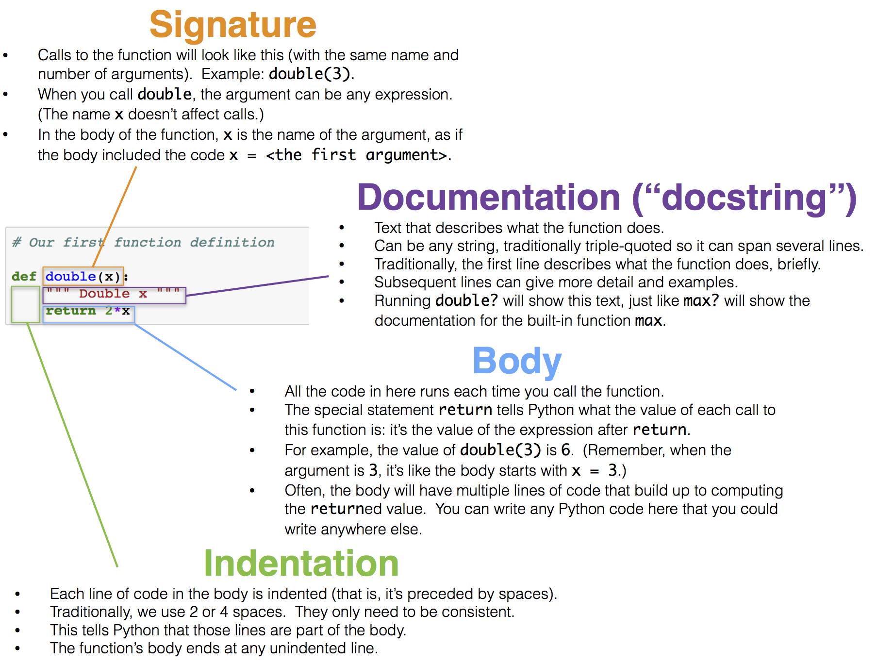
When we run the cell above, no particular number is doubled, and the code inside the body of double is not yet evaluated. In this respect, our function is analogous to a recipe. Each time we follow the instructions in a recipe, we need to start with ingredients. Each time we want to use our function to double a number, we need to specify a number.

We can call double in exactly the same way we have called other functions. Each time we do that, the code in the body is executed, with the value of the argument given the name x.

Python

double(17)
# 34

Python

double(-0.6/4)
# -0.3

The two expressions above are both call expressions. In the second one, the value of the expression -0.6/4 is computed and then passed as the argument named x to the double function. Each call expresson results in the body of double being executed, but with a different value of x.

The body of double has only a single line:

Python

return 2*x

Executing this return statement completes execution of the double function’s body and computes the value of the call expression.

The argument to double can be any expression, as long as its value is a number. For example, it can be a name. The double function does not know or care how its argument is computed or stored; its only job is to execute its own body using the values of the arguments passed to it.

Python

any_name = 42
double(any_name)
# 84

The argument can also be any value that can be doubled. For example, a whole array of numbers can be passed as an argument to double, and the result will be another array.

Python

import numpy as np

double(np.array([3, 4, 5]))
# array([ 6,  8, 10])

However, names that are defined inside a function, including arguments like double’s x, have only a fleeting existence. They are defined only while the function is being called, and they are only accessible inside the body of the function. We can’t refer to x outside the body of double. The technical terminology is that x has local scope.

Therefore the name x isn’t recognized outside the body of the function, even though we have called double in the cells above.

Python

x
# NameError: name 'x' is not defined

Docstrings. Though double is relatively easy to understand, many functions perform complicated tasks and are difficult to use without explanation. (You may have discovered this yourself!) Therefore, a well-composed function has a name that evokes its behavior, as well as documentation. In Python, this is called a docstring — a description of its behavior and expectations about its arguments. The docstring can also show example calls to the function, where the call is preceded by >>>.

A docstring can be any string, as long as it is the first thing in a function’s body. Docstrings are typically defined using triple quotation marks at the start and end, which allows a string to span multiple lines. The first line is conventionally a complete but short description of the function, while following lines provide further guidance to future users of the function.

Here is a definition of a function called percent that takes two arguments. The definition includes a docstring.

Python

# A function with more than one argument

def percent(x, total):
    """Convert x to a percentage of total.
    
    More precisely, this function divides x by total,
    multiplies the result by 100, and rounds the result
    to two decimal places.
    
    >>> percent(4, 16)
    25.0
    >>> percent(1, 6)
    16.67
    """
    return round((x/total)*100, 2)

Python

percent(33, 200)
# 16.5

Contrast the function percent defined above with the function percents defined below. The latter takes an array as its argument, and converts all the numbers in the array to percents out of the total of the values in the array. The percents are all rounded to two decimal places, this time replacing round by np.round because the argument is an array and not a number.

Python

def percents(counts):
    """Convert the values in array_x to percents out of the total of array_x."""
    total = counts.sum()
    return np.round((counts/total)*100, 2)

Python

some_array = np.array([7, 10, 4])
percents(some_array)
# array([33.33, 47.62, 19.05])

It is helpful to understand the steps Python takes to execute a function. To facilitate this, we have put a function definition and a call to that function in the same cell below.

Python

def biggest_difference(array_x):
    """Find the biggest difference in absolute value between two adjacent elements of array_x."""
    diffs = np.diff(array_x)
    absolute_diffs = abs(diffs)
    return max(absolute_diffs)

some_numbers = np.array([2, 4, 5, 6, 4, -1, 1])
big_diff = biggest_difference(some_numbers)
print("The biggest difference is", big_diff)
#The biggest difference is 5

Here is what happens when we run that cell:

---

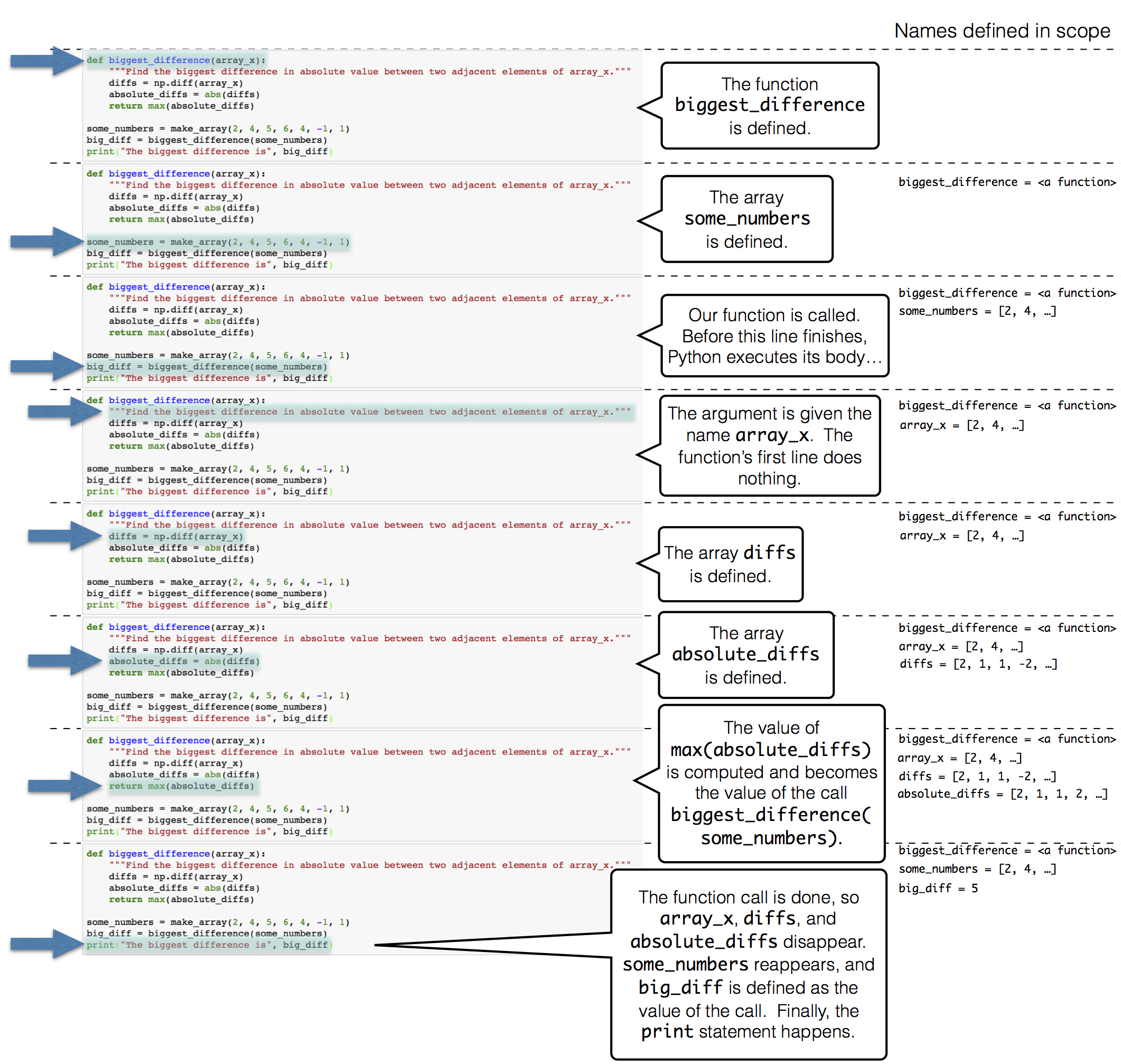
Multiple Arguments

There can be multiple ways to generalize an expression or block of code, and so a function can take multiple arguments that each determine different aspects of the result. For example, the percents function we defined previously rounded to two decimal places every time. The following two-argument definition allows different calls to round to different amounts.

Python

def percents(counts, decimal_places):
    """Convert the values in array_x to percents out of the total of array_x."""
    total = counts.sum()
    return np.round((counts/total)*100, decimal_places)

parts = np.array([2, 1, 4])
print("Rounded to 1 decimal place: ", percents(parts, 1))
print("Rounded to 2 decimal places:", percents(parts, 2))
print("Rounded to 3 decimal places:", percents(parts, 3))
'''
Rounded to 1 decimal place:  [28.6 14.3 57.1]
Rounded to 2 decimal places: [28.57 14.29 57.14]
Rounded to 3 decimal places: [28.571 14.286 57.143]
'''

The flexibility of this new definition comes at a small price: each time the function is called, the number of decimal places must be specified. Default argument values allow a function to be called with a variable number of arguments; any argument that isn’t specified in the call expression is given its default value, which is stated in the first line of the def statement. For example, in this final definition of percents, the optional argument decimal_places is given a default value of 2.

Python

def percents(counts, decimal_places=2):
    """Convert the values in array_x to percents out of the total of array_x."""
    total = counts.sum()
    return np.round((counts/total)*100, decimal_places)

parts = np.array([2, 1, 4])
print("Rounded to 1 decimal place:", percents(parts, 1))
print("Rounded to the default number of decimal places:", percents(parts))
'''
Rounded to 1 decimal place: [28.6 14.3 57.1]
Rounded to the default number of decimal places: [28.57 14.29 57.14]
'''

---

Note: Methods

Functions are called by placing argument expressions in parentheses after the function name. Any function that is defined in isolation is called in this way. You have also seen examples of methods, which are like functions but are called using dot notation, such as <df>.sort_values(by=["<col>"]). The functions that you define will always be called using the function name first, passing in all of the arguments.

---

Applying a Function to a Column

We have seen many examples of creating new columns of tables by applying functions to existing columns or to other arrays. All of those functions took arrays as their arguments. But frequently we will want to convert the entries in a column by a function that doesn’t take an array as its argument. For example, it might take just one number as its argument, as in the function cut_off_at_100 defined below.

Python

def cut_off_at_100(x):
    """The smaller of x and 100"""
    return min(x, 100)

Python

cut_off_at_100(17)
# 17

cut_off_at_100(117)
# 100

cut_off_at_100(100)
# 100

The function cut_off_at_100 simply returns its argument if the argument is less than or equal to 100. But if the argument is greater than 100, it returns 100.

In our earlier examples using Census data, we saw that the variable AGE had a value 100 that meant “100 years old or older”. Cutting off ages at 100 in this manner is exactly what cut_off_at_100 does.

To use this function on many ages at once, we will have to be able to refer to the function itself, without actually calling it. Analogously, we might show a cake recipe to a chef and ask her to use it to bake 6 cakes. In that scenario, we are not using the recipe to bake any cakes ourselves; our role is merely to refer the chef to the recipe. Similarly, we can ask a table to call cut_off_at_100 on 6 different numbers in a column.

First, we create the table ages with a column for people and one for their ages. For example, person C is 52 years old.

Python

ages = pd.DataFrame({'Person': np.array(['A', 'B', 'C', 'D', 'E', 'F']), 
                     'Age': np.array([17, 117, 52, 100, 6, 101])})
ages

	Person	Age
0	A	17
1	B	117
2	C	52
3	D	100
4	E	6
5	F	101

---

apply

pandas.DataFrame.apply

To cut off each of the ages at 100, we will use a new Pandas.DataFrame method. The apply method calls a function on each element of a column, forming a new array of return values. To indicate which function to call, just name it (without quotation marks or parentheses). The name of the column of input values is a string that must still appear within quotation marks.

Python

# Filter ages.Age by cut_off_at_100
# ages.Age.apply(cut_off_at_100)
ages['Age'].apply(cut_off_at_100)
'''
0     17
1    100
2     52
3    100
4      6
5    100
Name: Age, dtype: int64
'''

What we have done here is apply the function cut_off_at_100 to each value in the Age column of the table ages. The output is the array of corresponding return values of the function. For example, 17 stayed 17, 117 became 100, 52 stayed 52, and so on.

This array, which has the same length as the original Age column of the ages table, can be used as the values in a new column called Cut Off Age alongside the existing Person and Age columns.

Python

# Add a column 'Cut Off Age'
ages['Cut Off Age'] = ages['Age'].apply(cut_off_at_100)
ages

	Person	Age	Cut Off Age
0	A	17	17
1	B	117	100
2	C	52	52
3	D	100	100
4	E	6	6
5	F	101	100

---

Functions as Values

We’ve seen that Python has many kinds of values. For example, 6 is a number value, “cake” is a text value, Table() is an empty table, and ages is a name for a table value (since we defined it above).

In Python, every function, including cut_off_at_100, is also a value. It helps to think about recipes again. A recipe for cake is a real thing, distinct from cakes or ingredients, and you can give it a name like “Ani’s cake recipe.” When we defined cut_off_at_100 with a def statement, we actually did two separate things: we created a function that cuts off numbers at 100, and we gave it the name cut_off_at_100.

We can refer to any function by writing its name, without the parentheses or arguments necessary to actually call it. We did this when we called apply above. When we write a function’s name by itself as the last line in a cell, Python produces a text representation of the function, just like it would print out a number or a string value.

Python

cut_off_at_100
# <function __main__.cut_off_at_100(x)>

Notice that we did not write cut_off_at_100 with quotes (which is just a piece of text), or cut_off_at_100() (which is a function call, and an invalid one at that). We simply wrote cut_off_at_100 to refer to the function.

Just like we can define new names for other values, we can define new names for functions. For example, suppose we want to refer to our function as cut_off instead of cut_off_at_100. We can just write this:

Python

cut_off = cut_off_at_100

Now cut_off is a name for a function. It’s the same function as cut_off_at_100, so the printed value is exactly the same.

Python

cut_off
# <function __main__.cut_off_at_100(x)>

Let us see another application of apply.

---

Example: Prediction

Data Science is often used to make predictions about the future. If we are trying to predict an outcome for a particular individual – for example, how she will respond to a treatment, or whether he will buy a product – it is natural to base the prediction on the outcomes of other similar individuals.

Charles Darwin’s cousin Sir Francis Galton was a pioneer in using this idea to make predictions based on numerical data. He studied how physical characteristics are passed down from one generation to the next.

The data below are Galton’s carefully collected measurements on the heights of parents and their adult children. Each row corresponds to one adult child. The variables are a numerical code for the family, the heights (in inches) of the father and mother, a “midparent height” which is a weighted average 1 of the height of the two parents, the number of children in the family, as well as the child’s birth rank (1 = oldest), gender, and height.

Python

# Galton's data on heights of parents and their adult children
galton = pd.read_csv('https://raw.githubusercontent.com/ZacksAmber/Code/master/Data%20Science/Data8/Data%20Sets/galton.csv')
galton

	family	father	mother	midparentHeight	children	childNum	gender	childHeight
0	1	78.5	67.0	75.43	4	1	male	73.2
1	1	78.5	67.0	75.43	4	2	female	69.2
2	1	78.5	67.0	75.43	4	3	female	69.0
3	1	78.5	67.0	75.43	4	4	female	69.0
4	2	75.5	66.5	73.66	4	1	male	73.5
...	...	...	...	...	...	...	...	...
929	203	62.0	66.0	66.64	3	1	male	64.0
930	203	62.0	66.0	66.64	3	2	female	62.0
931	203	62.0	66.0	66.64	3	3	female	61.0
932	204	62.5	63.0	65.27	2	1	male	66.5
933	204	62.5	63.0	65.27	2	2	female	57.0

A primary reason for collecting the data was to be able to predict the adult height of a child born to parents similar to those in the dataset. Let us try to do this, using midparent height as the variable on which to base our prediction. Thus midparent height is our predictor variable.

The table heights consists of just the midparent heights and child’s heights. The scatter plot of the two variables shows a positive association, as we would expect for these variables.

Python

# Extract midparentHeight and childHeight from galton
heights = pd.DataFrame({'MidParent': galton.midparentHeight, 
                        'Child':galton.childHeight})
heights

	MidParent	Child
0	75.43	73.2
1	75.43	69.2
2	75.43	69.0
3	75.43	69.0
4	73.66	73.5
...	...	...
929	66.64	64.0
930	66.64	62.0
931	66.64	61.0
932	65.27	66.5
933	65.27	57.0

Python

# Scatter of Child vs. MidParent
fig = px.scatter(heights, 
                 x='MidParent', 
                 y='Child', 
                 color_discrete_sequence=['rgb(2, 21 ,51)'], 
                 opacity=0.7)
# Set layout
fig.update_layout(title='Scatter of Child vs. MidParent')

fig.show()
# fig.write_image('fig.svg')
# ![](https://raw.githubusercontent.com/ZacksAmber/PicGo/master/img/20210421225052.svg)

Now suppose Galton encountered a new couple, similar to those in his dataset, and wondered how tall their child would be. What would be a good way for him to go about predicting the child’s height, given that the midparent height was, say, 68 inches?

One reasonable approach would be to base the prediction on all the points that correspond to a midparent height of around 68 inches. The prediction equals the average child’s height calculated from those points alone.

Let’s pretend we are Galton and execute this plan. For now we will just make a reasonable definition of what “around 68 inches” means, and work with that. Later in the course we will examine the consequences of such choices.

We will take “close” to mean “within half an inch”. The figure below shows all the points corresponding to a midparent height between 67.5 inches and 68.5 inches. These are all the points in the strip between the red lines. Each of these points corresponds to one child; our prediction of the height of the new couple’s child is the average height of all the children in the strip. That’s represented by the gold dot.

Ignore the code, and just focus on understanding the mental process of arriving at that gold dot.

Shapes in Python
Styling Markers in Python

Python

# Add shape to fig
fig.add_shape(type='line', x0=67.5, y0=50, x1=67.5, y1=85, line_color='red')
fig.add_shape(type='line', x0=68.5, y0=50, x1=68.5, y1=85, line_color='red')

# Add marker to fig
fig.add_trace(
    go.Scatter(
        mode='markers',
        x=[68],
        y=[66.24],
        marker=dict(
            color='Gold',
            size=12,
        ),
        showlegend=False
    )
)

fig.show()
# fig.write_image('fig.svg', scale=2)
# ![](https://raw.githubusercontent.com/ZacksAmber/PicGo/master/img/20210331224256.svg)

In order to calculate exactly where the gold dot should be, we first need to indentify all the points in the strip. These correspond to the rows where MidParent is between 67.5 inches and 68.5 inches.

Python

# Filter the MidParent that between 67.5 and 68.5
filter = (67.5 <= heights['MidParent']) & (heights['MidParent'] <= 68.5)
close_to_68 = heights.loc[filter]
close_to_68

	MidParent	Child
233	68.44	62.0
396	67.94	71.2
397	67.94	67.0
516	68.33	62.5
517	68.23	73.0
...	...	...
885	67.60	69.0
886	67.60	68.0
887	67.60	67.7
888	67.60	64.5
889	67.60	60.5

The predicted height of a child who has a midparent height of 68 inches is the average height of the children in these rows. That’s 66.24 inches.

Python

# Average child's height of close_to_68
np.mean(close_to_68.Child)
# 66.24045801526718

We now have a way to predict the height of a child given any value of the midparent height near those in our dataset. We can define a function predict_child that does this. The body of the function consists of the code in the two cells above, apart from choices of names.

Python

# Define predict_child for predicting any value of the midparent height
def predict_child(mpht):
    """Predict the height of a child whose parents have a midparent height of mpht.
    
    The prediction is the average height of the children whose midparent height is
    in the range mpht plus or minus 0.5.
    """
    filter = (mpht-0.5 <= heights.MidParent) & (heights.MidParent <= mpht+0.5)
    close_points = heights.loc[filter]
    
    return np.mean(close_points.Child)

Python

predict_child(68)
# 66.24045801526718

predict_child(74)
# 70.41578947368421

How good are these predictions? We can get a sense of this by comparing the predictions with the data that we already have. To do this, we first apply the function predict_child to the column of Midparent heights, and collect the results in a new column called Prediction.

Python

# Apply predict_child to all the midparent heights
heights_with_predictions = heights.copy()
heights_with_predictions['Prediction'] = heights.MidParent.apply(predict_child)
heights_with_predictions

	MidParent	Child	Prediction
0	75.43	73.2	70.100000
1	75.43	69.2	70.100000
2	75.43	69.0	70.100000
3	75.43	69.0	70.100000
4	73.66	73.5	70.415789
...	...	...	...
929	66.64	64.0	65.156579
930	66.64	62.0	65.156579
931	66.64	61.0	65.156579
932	65.27	66.5	64.229630
933	65.27	57.0	64.229630

To see where the predictions lie relative to the observed data, we can draw overlaid scatter plots with MidParent as the common horizontal axis.

Scatter Plots in Python
plotly.graph_objects.Scatter

Python

# Draw the original scatter plot along with the predicted values
fig = go.Figure()

# Add trace Child
fig.add_trace(go.Scatter(
    mode='markers', 
    x=heights_with_predictions['MidParent'], 
    y=heights_with_predictions['Child'], 
    name='Child', 
    marker_color='rgba(2, 21 ,51, .8)')) # rgb + opacity

# Add trace Prediction
fig.add_trace(go.Scatter(
    mode='markers', 
    x=heights_with_predictions['MidParent'], 
    y=heights_with_predictions['Prediction'], 
    name='Predication', 
    marker_color='rgba(250, 211, 102, .8)')) # rgb + opacity

# Set layout
fig.update_layout(title="Prediction of Children's heights", 
                  xaxis_title='MidParent', 
                  yaxis_title='')

fig.show()
# fig.write_image('fig.svg')
# ![](https://raw.githubusercontent.com/ZacksAmber/PicGo/master/img/20210422011901.svg)

The graph of gold dots is called a graph of averages, because each gold dot is the center of a vertical strip like the one we drew earlier. Each one provides a prediction of a child’s height given the midparent height. For example, the scatter shows that for a midparent height of 72 inches, the predicted height of the child would be somewhere between 68 inches and 69 inches, and indeed predict_child(72) returns 68.5.

Galton’s calculations and visualizations were very similar to ours, except that he didn’t have Python. He drew the graph of averages through the scatter diagram and noticed that it roughly followed a straight line. This straight line is now called the regression line and is one of the most common methods of making predictions. Galton’s friend, the mathematician Karl Pearson, used these analyses to formalize the notion of correlation.

This example, like the one about John Snow’s analysis of cholera deaths, shows how some of the fundamental concepts of modern data science have roots going back more than a century. Galton’s methods such as the one we have used here are precursors to nearest neighbor prediction methods that now have powerful applications in diverse settings. The modern field of machine learning includes the automation of such methods to make predictions based on vast and rapidly evolving datasets.

---

Classifying by One Variable

Data scientists often need to classify individuals into groups according to shared features, and then identify some characteristics of the groups. For example, in the example using Galton’s data on heights, we saw that it was useful to classify families according to the parents’ midparent heights, and then find the average height of the children in each group.

This section is about classifying individuals into categories that are not numerical. We begin by recalling the basic use of group.

---

Counting the Number in Each Category

The groupby method with a single argument counts the number of rows for each category in a column. The result contains one row per unique value in the grouped column.

Here is a small table of data on ice cream cones. The group method can be used to list the distinct flavors and provide the counts of each flavor.

Python

# Create DataFrame
cones = pd.DataFrame(
    {'Flavor': np.array(['strawberry', 'chocolate', 'chocolate', 'strawberry', 'chocolate']),
    'Price': np.array([3.55, 4.75, 6.55, 5.25, 5.25])}
)
cones

	Flavor	Price
0	strawberry	3.55
1	chocolate	4.75
2	chocolate	6.55
3	strawberry	5.25
4	chocolate	5.25

Group by: split-apply-combine
pandas.DataFrame.size

Python

# Draw pivot table, group by size or count
cones.groupby('Flavor').size().reset_index(name='count')
# OR
# cones.groupby('Flavor')['Flavor'].count().reset_index(name='count')

	Flavor	count
0	chocolate	3
1	strawberry	2

There are two distinct categories, chocolate and strawberry. The call to group creates a table of counts in each category. The column is called count by default, and contains the number of rows in each category.

Notice that this can all be worked out from just the Flavor column. The Price column has not been used.

But what if we wanted the total price of the cones of each different flavor? That’s where the second argument of group comes in.

---

Finding a Characteristic of Each Category

The optional second argument of groupby names the function that will be used to aggregate values in other columns for all of those rows. For instance, sum will sum up the prices in all rows that match each category. This result also contains one row per unique value in the grouped column, but it has the same number of columns as the original table.

To find the total price of each flavor, we call groupby again, with Flavor as its first argument as before. But this time there is a second argument: the function name sum.

Python

# SELECT Flavor, SUM(Price) AS 'Price sum' FROM cones;
cones.groupby('Flavor').sum('Price')['Price'].reset_index(name='Price sum')

	Flavor	Price sum
0	chocolate	16.55
1	strawberry	8.80

To create this new table, groupby has calculated the sum of the Price entries in all the rows corresponding to each distinct flavor. The prices in the three chocolate rows add up to $16.55 (you can assume that price is being measured in dollars).

The prices in the two strawberry rows have a total of $8.80.

The label of the newly created “sum” column is Price sum, which is created by taking the label of the column being summed, and appending the word sum.

Because groupby finds the sum of all columns other than the one with the categories, there is no need to specify that it has to sum the prices.

To see in more detail what groupby is doing, notice that you could have figured out the total prices yourself, not only by mental arithmetic but also using code. For example, to find the total price of all the chocolate cones, you could start by creating a new table consisting of only the chocolate cones, and then accessing the column of prices:

Python

# SELECT Price FROM cones WHERE 'Flavor' = 'chocolate';
cones[cones['Flavor'] == 'chocolate'].Price
'''
1    4.75
2    6.55
4    5.25
Name: Price, dtype: float64
'''

Python

# Sum all the price of chocolate
sum(cones[cones['Flavor'] == 'chocolate'].Price)
# 16.55

This is what group is doing for each distinct value in Flavor.

Python

# SELECT Price FROM cones WHERE Flavor = 'chocolate';
cones_choc = cones[cones['Flavor'] == 'chocolate'].Price

# SELECT Price FROM cones WHERE Flavor = 'strawberry';
cones_strawb = cones[cones['Flavor'] == 'strawberry'].Price

# Make DataFrame
grouped_cones = pd.DataFrame(
    {'Flavor': np.array(['chocolate', 'strawberry']),
    'Array of All the Prices': [np.array(cones_choc), np.array(cones_strawb)]}
)

# Append a column with the sum of the `Price` values in each array
price_totals = grouped_cones.copy()
price_totals['Sum of the Array'] = [np.sum(cones_choc), np.sum(cones_strawb)]

price_totals

	Flavor	Array of All the Prices	Sum of the Array
0	chocolate	[4.75, 6.55, 5.25]	16.55
1	strawberry	[3.55, 5.25]	8.80

You can replace sum by any other functions that work on arrays. For example, you could use max to find the largest price in each category:

pandas.core.groupby.GroupBy.max

Python

# SELECT Flavor, MAX('Price') AS 'Price Max' FROM cones GROUP BY 'Flavor';
cones.groupby('Flavor').max('Price')['Price'].reset_index(name='Price Max')

	Flavor	Price Max
0	chocolate	6.55
1	strawberry	5.25

Once again, groupby creates arrays of the prices in each Flavor category. But now it finds the max of each array:

Python

# Create a new DataFrame Price_maxes from grouped_cones. Then add a new column 'Max of the Array'
price_maxes = grouped_cones.copy()
price_maxes['Max of the Array'] = [np.max(cones_choc), np.max(cones_strawb)]
price_maxes

	Flavor	Array of All the Prices	Max of the Array
0	chocolate	[4.75, 6.55, 5.25]	6.55
1	strawberry	[3.55, 5.25]	5.25

Indeed, the original call to groupby with just one argument has the same effect as using len as the function and then cleaning up the table.

Python

# Create a new DataFrame lengths from grouped_cones. Then add a new column 'Length of the Array'
lengths = grouped_cones.copy()
lengths['Length of the Array'] = [len(cones_choc), len(cones_strawb)]
lengths

	Flavor	Array of All the Prices	Length of the Array
0	chocolate	[4.75, 6.55, 5.25]	3
1	strawberry	[3.55, 5.25]	2

---

Example: NBA Salaries

The table nba contains data on the 2015-2016 players in the National Basketball Association. We have examined these data earlier. Recall that salaries are measured in millions of dollars.

Python

# Read CSV nba_salaries.csv
nba1 = pd.read_csv('https://github.com/ZacksAmber/Code/raw/master/Data%20Science/Data8/Data%20Sets/nba_salaries.csv')
nba = nba1.rename(columns={"'15-'16 SALARY": 'SALARY'})
nba

	PLAYER	POSITION	TEAM	SALARY
0	Paul Millsap	PF	Atlanta Hawks	18.671659
1	Al Horford	C	Atlanta Hawks	12.000000
2	Tiago Splitter	C	Atlanta Hawks	9.756250
3	Jeff Teague	PG	Atlanta Hawks	8.000000
4	Kyle Korver	SG	Atlanta Hawks	5.746479
...	...	...	...	...
412	Gary Neal	PG	Washington Wizards	2.139000
413	DeJuan Blair	C	Washington Wizards	2.000000
414	Kelly Oubre Jr.	SF	Washington Wizards	1.920240
415	Garrett Temple	SG	Washington Wizards	1.100602
416	Jarell Eddie	SG	Washington Wizards	0.561716

1. How much money did each team pay for its players’ salaries?

The only columns involved are TEAM and SALARY. We have to group the rows by TEAM and then sum the salaries of the groups.

Python

# Q: How much money did each team pay for its players’ salaries?
nba.groupby('TEAM').sum('SALARY')['SALARY'].reset_index(name='SALARY sum')

	TEAM	SALARY sum
0	Atlanta Hawks	69.573103
1	Boston Celtics	50.285499
2	Brooklyn Nets	57.306976
3	Charlotte Hornets	84.102397
4	Chicago Bulls	78.820890
...	...	...
25	Sacramento Kings	68.384890
26	San Antonio Spurs	84.652074
27	Toronto Raptors	74.672620
28	Utah Jazz	52.631878
29	Washington Wizards	90.047498

2. How many NBA players were there in each of the five positions?

We have to classify by POSITION, and count. This can be done with just one argument to group:

Python

# Q: How many NBA players were there in each of the five positions?
nba.groupby('POSITION')['POSITION'].count().reset_index(name='count')

	POSITION	count
0	C	69
1	PF	85
2	PG	85
3	SF	82
4	SG	96

3. What was the average salary of the players at each of the five positions?

This time, we have to group by POSITION and take the mean of the salaries. For clarity, we will work with a table of just the positions and the salaries.

Python

# Q3: What was the average salary of the players at each of the five positions?
nba.groupby('POSITION')['SALARY'].mean('SALARY').reset_index(name='SALARY mean')

	POSITION	SALARY mean
0	C	6.082913
1	PF	4.951344
2	PG	5.165487
3	SF	5.532675
4	SG	3.988195

Center was the most highly paid position, at an average of over 6 million dollars.

---

Cross-Classifying by More than One Variable

When individuals have multiple features, there are many different ways to classify them. For example, if we have a population of college students for each of whom we have recorded a major and the number of years in college, then the students could be classified by major, or by year, or by a combination of major and year.

The group method also allows us to classify individuals according to multiple variables. This is called cross-classifying.

---

Two Variables: Counting the Number in Each Paired Category

The table more_cones records the flavor, color, and price of six ice cream cones.

Python

# Create a DataFrame more_cones
more_cones = pd.DataFrame(
    {'Flavor': np.array(['strawberry', 'chocolate', 'chocolate', 'strawberry', 'chocolate', 'bubblegum']),
    'Color': np.array(['pink', 'light brown', 'dark brown', 'pink', 'dark brown', 'pink']),
    'Price': np.array([3.55, 4.75, 5.25, 5.25, 5.25, 4.75])}
)

more_cones

	Flavor	Color	Price
0	strawberry	pink	3.55
1	chocolate	light brown	4.75
2	chocolate	dark brown	5.25
3	strawberry	pink	5.25
4	chocolate	dark brown	5.25
5	bubblegum	pink	4.75

We know how to use groupby to count the number of cones of each flavor:

Python

# SELECT Flavor, COUNT(*) AS count FROM more_cones GROUP BY Flavor;
more_cones.groupby('Flavor')['Flavor'].count().reset_index(name='count')

	Flavor	count
0	bubblegum	1
1	chocolate	3
2	strawberry	2

But now each cone has a color as well. To classify the cones by both flavor and color, we will pass a list of labels as an argument to group. The resulting table has one row for every unique combination of values that appear together in the grouped columns. As before, a single argument (a list, in this case, but an array would work too) gives row counts.

Although there are six cones, there are only four unique combinations of flavor and color. Two of the cones were dark brown chocolate, and two pink strawberry.

Python

# SELECT Flavor, COUNT(*) AS count FROM more_cones GROUP BY Flavor, Color;
more_cones.groupby(['Flavor', 'Color'])['Flavor'].count().reset_index(name='count')

	Flavor	Color	count
0	bubblegum	pink	1
1	chocolate	dark brown	2
2	chocolate	light brown	1
3	strawberry	pink	2

---

Two Variables: Finding a Characteristic of Each Paired Category

A second argument aggregates all other columns that are not in the list of grouped columns.

Python

# SELECT Flavor, SUM(Price) AS 'Price sum' FROM more_cones GROUP BY Flavor, Color;
more_cones.groupby(['Flavor', 'Color'])['Price'].sum('Price').reset_index(name='Price sum')

	Flavor	Color	Price sum
0	bubblegum	pink	4.75
1	chocolate	dark brown	10.50
2	chocolate	light brown	4.75
3	strawberry	pink	8.80

Three or More Variables. You can use groupby to classify rows by three or more categorical variables. Just include them all in the list that is the first argument. But cross-classifying by multiple variables can become complex, as the number of distinct combinations of categories can be quite large.

---

Pivot Tables: Rearranging the Output of group

pandas.DataFrame.pivot
pandas.DataFrame.pivot_table
Reshaping and pivot tables

Many uses of cross-classification involve just two categorical variables, like Flavor and Color in the example above. In these cases it is possible to display the results of the classification in a different kind of table, called a pivot table. Pivot tables, also known as contingency tables, make it easier to work with data that have been classified according to two variables.

Recall the use of group to count the number of cones in each paired category of flavor and color:

Python

# SELECT Flavor, COUNT(*) AS count FROM more_cones GROUP BY Flavor, Color;
more_cones.groupby(['Flavor', 'Color'])['Flavor'].count().reset_index(name='count')

	Flavor	Color	count
0	bubblegum	pink	1
1	chocolate	dark brown	2
2	chocolate	light brown	1
3	strawberry	pink	2

The same data can be displayed differenly using the Pandas method pivot_table. Ignore the code for a moment, and just examine the table of outcomes.

Python

# Pivot Table
pd.pivot_table(more_cones, 
               index=['Color'], 
               columns=['Flavor'], 
               aggfunc='count', 
               fill_value=0).rename(columns={'Price': ''})

Flavor	bubblegum	chocolate	strawberry
Color
dark brown	0	2	0
light brown	0	1	0
pink	1	0	2

Notice how this table displays all nine possible pairs of Flavor and Color, including pairs like “dark brown bubblegum” that don’t exist in our data. Notice also that the count in each pair appears in the body of the table: to find the number of light brown chocolate cones, run your eye along the row light brown until it meets the column chocolate.

The groupby method takes a list of two labels because it is flexible: it could take one or three or more. On the other hand, pivot always takes two column labels, one to determine the columns and one to determine the rows.

pitvot_table

The pitvot_table method is closely related to the groupby method: it groups together rows that share a combination of values. It differs from group because it organizes the resulting values in a grid. The first argument to pivot is the label of a column that contains the values that will be used to form new columns in the result. The second argument is the label of a column used for the rows. The result gives the count of all rows of the original table that share the combination of column and row values.

Like groupby, pitvot_table can be used with additional arguments to find characteristics of each paired category. An optional third argument called values indicates a column of values that will replace the counts in each cell of the grid. All of these values will not be displayed, however; the fourth argument collect indicates how to collect them all into one aggregated value to be displayed in the cell.

An example will help clarify this. Here is pitvot_table being used to find the total price of the cones in each cell.

Python

# Pivot Table
pd.pivot_table(more_cones, 
               index=['Color'], 
               columns=['Flavor'],
               values=['Price'], 
               aggfunc='sum', 
               fill_value=0).rename(columns={'Price': ''})

Flavor	bubblegum	chocolate	strawberry
Color
dark brown	0.00	10.50	0.0
light brown	0.00	4.75	0.0
pink	4.75	0.00	8.8

And here is group doing the same thing.

Python

# SELECT Flavor, Color, SUM(Price) AS 'Price sum' FROM more_cones GROUP BY Flavor, Color;
more_cones.groupby(['Flavor', 'Color'])['Price'].sum().reset_index(name='Price sum')

	Flavor	Color	Price sum
0	bubblegum	pink	4.75
1	chocolate	dark brown	10.50
2	chocolate	light brown	4.75
3	strawberry	pink	8.80

Though the numbers in both tables are the same, table produced by pivot_table is easier to read and lends itself more easily to analysis. The advantage of pivot is that it places grouped values into adjacent columns, so that they can be combined and compared.

---

Example: Education and Income of Californian Adults

The State of California’s Open Data Portal is a rich source of information about the lives of Californians. It is our source of a dataset on educational attainment and personal income among Californians over the years 2008 to 2014. The data are derived from the U.S. Census Current Population Survey.

For each year, the table records the Population Count of Californians in many different combinations of age, gender, educational attainment, and personal income. We will study only the data for the year 2014

Python

# Read CSV educ_inc.csv
full_table = pd.read_csv('https://raw.githubusercontent.com/ZacksAmber/Code/master/Data%20Science/Data8/Data%20Sets/educ_inc.csv')
ca_2014 = full_table.loc[(full_table['Year'] == '1/1/14 0:00') & (full_table['Age'] != '00 to 17')]
ca_2014

	Year	Age	Gender	Educational Attainment	Personal Income	Population Count
885	1/1/14 0:00	18 to 64	Female	No high school diploma	H: 75,000 and over	2058
886	1/1/14 0:00	65 to 80+	Male	No high school diploma	H: 75,000 and over	2153
894	1/1/14 0:00	65 to 80+	Female	No high school diploma	G: 50,000 to 74,999	4666
895	1/1/14 0:00	65 to 80+	Female	High school or equivalent	H: 75,000 and over	7122
896	1/1/14 0:00	65 to 80+	Female	No high school diploma	F: 35,000 to 49,999	7261
...	...	...	...	...	...	...
1021	1/1/14 0:00	18 to 64	Female	High school or equivalent	A: 0 to 4,999	670294
1022	1/1/14 0:00	18 to 64	Male	Bachelor's degree or higher	G: 50,000 to 74,999	682425
1023	1/1/14 0:00	18 to 64	Female	No high school diploma	A: 0 to 4,999	723208
1024	1/1/14 0:00	18 to 64	Female	Bachelor's degree or higher	H: 75,000 and over	953282
1025	1/1/14 0:00	18 to 64	Male	Bachelor's degree or higher	H: 75,000 and over	1628605

Each row of the table corresponds to a combination of age, gender, educational level, and income. There are 127 such combinations in all!

As a first step it is a good idea to start with just one or two variables. We will focus on just one pair: educational attainment and personal income.

Python

# Filter 'Educational Attainment', 'Personal Income', 'Population Count'
educ_inc = ca_2014.loc[:, ['Educational Attainment', 'Personal Income', 'Population Count']]
educ_inc

	Educational Attainment	Personal Income	Population Count
885	No high school diploma	H: 75,000 and over	2058
886	No high school diploma	H: 75,000 and over	2153
894	No high school diploma	G: 50,000 to 74,999	4666
895	High school or equivalent	H: 75,000 and over	7122
896	No high school diploma	F: 35,000 to 49,999	7261
...	...	...	...
1021	High school or equivalent	A: 0 to 4,999	670294
1022	Bachelor's degree or higher	G: 50,000 to 74,999	682425
1023	No high school diploma	A: 0 to 4,999	723208
1024	Bachelor's degree or higher	H: 75,000 and over	953282
1025	Bachelor's degree or higher	H: 75,000 and over	1628605

Let’s start by looking at educational level alone. The categories of this variable have been subdivided by the different levels of income. So we will group the table by Educational Attainment and sum the Population Count in each category.

Python

# Filter 'Educational Attainment', 'Population Count'
education = educ_inc.loc[:, ['Educational Attainment', 'Population Count']]

# SELECT 'Educational Attainment', SUM('Population Count') AS 'Population Count sum' FROM educ_totals GROUP BY 'Educational Attainment';
educ_totals = education.groupby('Educational Attainment')['Population Count'].sum().reset_index(name='Population Count sum')
educ_totals

	Educational Attainment	Population Count sum
0	Bachelor's degree or higher	8525698
1	College, less than 4-yr degree	7775497
2	High school or equivalent	6294141
3	No high school diploma	4258277

There are only four categories of educational attainment. The counts are so large that is is more helpful to look at percents. For this, we will use the function percents that we defined in an earlier section. It converts an array of numbers to an array of percents out of the total in the input array.

Python

def percents(array_x):
    return np.round( (array_x/sum(array_x))*100, 2)

We now have the distribution of educational attainment among adult Californians. More than 30% have a Bachelor’s degree or higher, while almost 16% lack a high school diploma.

Python

# Copy educ_totals to educ_distribution. Then add a column to it.
educ_distribution = educ_totals.copy()
educ_distribution['Population Percent'] = percents(educ_distribution.iloc[:, 1])
educ_distribution

	Educational Attainment	Population Count sum	Population Percent
0	Bachelor's degree or higher	8525698	31.75
1	College, less than 4-yr degree	7775497	28.96
2	High school or equivalent	6294141	23.44
3	No high school diploma	4258277	15.86

By using pivot_table, we can get a contingency table (a table of counts) of adult Californians cross-classified by Educational Attainment and Personal Income.

Python

# Pivot Table
total = pd.pivot_table(educ_inc, 
                       index=['Personal Income'], 
                       columns=['Educational Attainment'], 
                       values=['Population Count'], 
                       aggfunc='sum').rename(columns={'Population Count': ''})
total

Here you see the power of pivot_table over other cross-classification methods. Each column of counts is a distribution of personal income at a specific level of educational attainment. Converting the counts to percents allows us to compare the four distributions.

Python

# Convert population of table total from numeric to percent
distributions = pd.DataFrame(
    {"Bachelor's degree or higher": percents(total.iloc[:, 0]), 
     'College, less than 4-yr degree': percents(total.iloc[:, 1]), 
     'High school or equivalent': percents(total.iloc[:, 2]), 
     'No high school diploma': percents(total.iloc[:, 3])}).reset_index()
distributions

	Personal Income	Bachelor's degree or higher	College, less than 4-yr degree	High school or equivalent	No high school diploma
0	A: 0 to 4,999	6.75	12.67	18.46	28.29
1	B: 5,000 to 9,999	3.82	10.43	9.95	14.02
2	C: 10,000 to 14,999	5.31	10.27	11.00	15.61
3	D: 15,000 to 24,999	9.07	17.30	19.90	20.56
4	E: 25,000 to 34,999	8.14	14.04	14.76	10.91
5	F: 35,000 to 49,999	13.17	14.31	12.44	6.12
6	G: 50,000 to 74,999	18.70	11.37	8.35	3.11
7	H: 75,000 and over	35.03	9.62	5.13	1.38

At a glance, you can see that over 35% of those with Bachelor’s degrees or higher had incomes of $75,000 and over, whereas fewer than 10% of the people in the other education categories had that level of income.

The bar chart below compares the personal income distributions of adult Californians who have no high school diploma with those who have completed a Bachelor’s degree or higher. The difference in the distributions is striking. There is a clear positive association between educational attainment and personal income.

layout.xaxis

Python

# Bar chart
fig = px.bar(distributions, 
             x=["Bachelor's degree or higher", 'No high school diploma'], 
             y='Personal Income', 
             barmode='group',
             color_discrete_sequence=['#636EFA', 'gold'])
# Change fig yaxis order
fig.update_layout(yaxis={'categoryorder': 'category descending'})
fig.show()
# fig.write_image('fig.svg', scale=2)
# ![](https://raw.githubusercontent.com/ZacksAmber/PicGo/master/img/20210401195101.svg)

---

Joining Tables by Columns

Often, data about the same individuals is maintained in more than one table. For example, one university office might have data about each student’s time to completion of degree, while another has data about the student’s tuition and financial aid.

To understand the students’ experience, it may be helpful to put the two datasets together. If the data are in two tables, each with one row per student, then we would want to put the columns together, making sure to match the rows so that each student’s information remains on a single row.

Let us do this in the context of a simple example, and then use the method with a larger dataset.

The table cones is one we have encountered earlier. Now suppose each flavor of ice cream comes with a rating that is in a separate table.

Python

# Create DataFrame cones
cones = pd.DataFrame(
    {'Flavor': np.array(['strawberry', 'vanilla', 'chocolate', 'strawberry', 'chocolate']),
    'Price': np.array([3.55, 4.75, 6.55, 5.25, 5.75])}
)
cones

	Flavor	Price
0	strawberry	3.55
1	vanilla	4.75
2	chocolate	6.55
3	strawberry	5.25
4	chocolate	5.75

Python

# Create DataFrame ratings
ratings = pd.DataFrame(
    {'Kind': np.array(['strawberry', 'chocolate', 'vanilla']),
    'Stars': np.array([2.5, 3.5, 4])}
)
ratings

	Kind	Stars
0	strawberry	2.5
1	chocolate	3.5
2	vanilla	4.0

Each of the tables has a column that contains ice cream flavors: cones has the column Flavor, and ratings has the column Kind. The entries in these columns can be used to link the two tables.

The method join creates a new table in which each cone in the cones table is augmented with the Stars information in the ratings table. For each cone in cones, join finds a row in ratings whose Kind matches the cone’s Flavor. We have to tell join to use those columns for matching.

pandas.DataFrame.join

Python

# Join table cones and ratings
rated = cones.join(ratings.set_index(['Kind']), on=['Flavor'])
rated

	Flavor	Price	Stars
0	strawberry	3.55	2.5
1	vanilla	4.75	4.0
2	chocolate	6.55	3.5
3	strawberry	5.25	2.5
4	chocolate	5.75	3.5

Each cone now has not only its price but also the rating of its flavor.

In general, a call to join that augments a table (say table1) with information from another table (say table2) looks like this:

Python

DataFrame.join(other, on=None, how='left', lsuffix='', rsuffix='', sort=False

The new table rated allows us to work out the price per star, which you can think of as an informal measure of value. Low values are good – they mean that you are paying less for each rating star.

Python

# Add a new column '$/Star' to table rated
rated['$/Star'] = round(rated.Price / rated.Stars, 3)
# Sort rated by '$/Star' ascending
rated.sort_values(by=['$/Star'], ascending=True)

	Flavor	Price	Stars	$/Star
1	vanilla	4.75	4.0	1.188
0	strawberry	3.55	2.5	1.420
4	chocolate	5.75	3.5	1.643
2	chocolate	6.55	3.5	1.871
3	strawberry	5.25	2.5	2.100

Though strawberry has the lowest rating among the three flavors, the less expensive strawberry cone does well on this measure because it doesn’t cost a lot per star.

Side note. Does the order we list the two tables matter? Let’s try it. As you see it, this changes the order that the columns appear in, and can potentially changes the order of the rows, but it doesn’t make any fundamental difference.

Python

# Join table cones and ratings
ratings.join(cones.set_index(['Flavor']), on=['Kind'])

	Kind	Stars	Price
0	strawberry	2.5	3.55
0	strawberry	2.5	5.25
1	chocolate	3.5	6.55
1	chocolate	3.5	5.75
2	vanilla	4.0	4.75

Also note that the join will only contain information about items that appear in both tables. Let’s see an example. Suppose there is a table of reviews of some ice cream cones, and we have found the average review for each flavor.

Python

# Create DataFrame reviews
reviews = pd.DataFrame(
    {'Flavor': ['vanilla', 'chocolate', 'vanilla', 'chocolate'],
    'Stars': [5, 3, 5, 4]}
)
reviews

	Flavor	Stars
0	vanilla	5
1	chocolate	3
2	vanilla	5
3	chocolate	4

Python

# SELECT Flavor, AVG(Stars) AS 'Stars Average' FROM reviews GROUP BY Flavor;
average_review = reviews.groupby('Flavor')['Stars'].mean().reset_index(name='Stars Average')
average_review

	Flavor	Stars Average
0	chocolate	3.5
1	vanilla	5.0

We can join cones and average_review by providing the labels of the columns by which to join.

pandas.DataFrame.join

Python

# SELECT Flavor, Price, 'Stars Average' FROM cones LEFT JOIN average_review USING('Flavor');
cones.join(average_review.set_index('Flavor'), on='Flavor', how='left')

	Flavor	Price	Stars Average
0	strawberry	3.55	NaN
1	vanilla	4.75	5.0
2	chocolate	6.55	3.5
3	strawberry	5.25	NaN
4	chocolate	5.75	3.5

Python

# SELECT Flavor, Price, 'Stars Average' FROM cones INNER JOIN average_review USING('Flavor');
cones.join(average_review.set_index('Flavor'), on='Flavor', how='inner')

	Flavor	Price	Stars Average
1	vanilla	4.75	5.0
2	chocolate	6.55	3.5
4	chocolate	5.75	3.5

Notice how the strawberry cones have disappeared. None of the reviews are for strawberry cones, so there is nothing to which the strawberry rows can be joined. This might be a problem, or it might not be - that depends on the analysis we are trying to perform with the joined table.

---

Bike Sharing in the Bay Area

We end this chapter by using all the methods we have learned to examine a new and large dataset.

The Bay Area Bike Share service published a dataset describing every bicycle rental from September 2014 to August 2015 in their system. There were 354,152 rentals in all. The columns are:

• An ID for the rental
• Duration of the rental, in seconds
• Start date
• Name of the Start Station and code for Start Terminal
• Name of the End Station and code for End Terminal
• A serial number for the bike
• Subscriber type and zip code

Python

 Read CSV trip.csv
trip = pd.read_csv('https://raw.githubusercontent.com/ZacksAmber/Code/master/Data%20Science/Data8/Data%20Sets/trip.csv')
trip

	Trip ID	Duration	Start Date	Start Station	Start Terminal	End Date	End Station	End Terminal	Bike #	Subscriber Type	Zip Code
0	913460	765	8/31/2015 23:26	Harry Bridges Plaza (Ferry Building)	50	8/31/2015 23:39	San Francisco Caltrain (Townsend at 4th)	70	288	Subscriber	2139
1	913459	1036	8/31/2015 23:11	San Antonio Shopping Center	31	8/31/2015 23:28	Mountain View City Hall	27	35	Subscriber	95032
2	913455	307	8/31/2015 23:13	Post at Kearny	47	8/31/2015 23:18	2nd at South Park	64	468	Subscriber	94107
3	913454	409	8/31/2015 23:10	San Jose City Hall	10	8/31/2015 23:17	San Salvador at 1st	8	68	Subscriber	95113
4	913453	789	8/31/2015 23:09	Embarcadero at Folsom	51	8/31/2015 23:22	Embarcadero at Sansome	60	487	Customer	9069
...	...	...	...	...	...	...	...	...	...	...	...
354147	432951	619	9/1/2014 4:21	Powell Street BART	39	9/1/2014 4:32	Townsend at 7th	65	335	Subscriber	94118
354148	432950	6712	9/1/2014 3:16	Harry Bridges Plaza (Ferry Building)	50	9/1/2014 5:08	San Francisco Caltrain (Townsend at 4th)	70	259	Customer	44100
354149	432949	538	9/1/2014 0:05	South Van Ness at Market	66	9/1/2014 0:14	5th at Howard	57	466	Customer	32
354150	432948	568	9/1/2014 0:05	South Van Ness at Market	66	9/1/2014 0:15	5th at Howard	57	461	Customer	32
354151	432947	569	9/1/2014 0:05	South Van Ness at Market	66	9/1/2014 0:15	5th at Howard	57	318	Customer	32

We’ll focus only on the free trips, which are trips that last less than 1800 seconds (half an hour). There is a charge for longer trips.

Python

# Filter the free trips
commute = trip[trip.Duration < 1800]
commute

	Trip ID	Duration	Start Date	Start Station	Start Terminal	End Date	End Station	End Terminal	Bike #	Subscriber Type	Zip Code
0	913460	765	8/31/2015 23:26	Harry Bridges Plaza (Ferry Building)	50	8/31/2015 23:39	San Francisco Caltrain (Townsend at 4th)	70	288	Subscriber	2139
1	913459	1036	8/31/2015 23:11	San Antonio Shopping Center	31	8/31/2015 23:28	Mountain View City Hall	27	35	Subscriber	95032
2	913455	307	8/31/2015 23:13	Post at Kearny	47	8/31/2015 23:18	2nd at South Park	64	468	Subscriber	94107
3	913454	409	8/31/2015 23:10	San Jose City Hall	10	8/31/2015 23:17	San Salvador at 1st	8	68	Subscriber	95113
4	913453	789	8/31/2015 23:09	Embarcadero at Folsom	51	8/31/2015 23:22	Embarcadero at Sansome	60	487	Customer	9069
...	...	...	...	...	...	...	...	...	...	...	...
354146	432952	240	9/1/2014 4:59	South Van Ness at Market	66	9/1/2014 5:03	Civic Center BART (7th at Market)	72	292	Subscriber	94102
354147	432951	619	9/1/2014 4:21	Powell Street BART	39	9/1/2014 4:32	Townsend at 7th	65	335	Subscriber	94118
354149	432949	538	9/1/2014 0:05	South Van Ness at Market	66	9/1/2014 0:14	5th at Howard	57	466	Customer	32
354150	432948	568	9/1/2014 0:05	South Van Ness at Market	66	9/1/2014 0:15	5th at Howard	57	461	Customer	32
354151	432947	569	9/1/2014 0:05	South Van Ness at Market	66	9/1/2014 0:15	5th at Howard	57	318	Customer	32

The histogram below shows that most of the trips took around 10 minutes (600 seconds) or so. Very few took near 30 minutes (1800 seconds), possibly because people try to return the bikes before the cutoff time so as not to have to pay.

Python

# Histogram, percent, bins=10
fig = px.histogram(commute, 
                   histnorm='percent', 
                   x='Duration', 
                   nbins=10)
fig.update_layout(xaxis_title='Duration (Second)', 
                  yaxis_title='Percent per Second')
fig.show()
# fig.write_image('fig.svg', scale=2)
# ![](https://raw.githubusercontent.com/ZacksAmber/PicGo/master/img/20210401225456.svg)

We can get more detail by specifying a larger number of bins. But the overall shape doesn’t change much.

Python

# Histogram, percent, bins=100
fig = px.histogram(commute, 
                   histnorm='percent', 
                   x='Duration', 
                   nbins=100)
fig.update_layout(xaxis_title='Duration (Second)', 
                  yaxis_title='Percent per Second')
fig.show()
# fig.write_image('fig.svg', scale=2)
# ![](https://raw.githubusercontent.com/ZacksAmber/PicGo/master/img/20210401225704.svg)

---

Exploring the Data with group and pivot

We can use group to identify the most highly used Start Station:

Python

# SELECT 'Start Station', COUNT(*) AS 'count' FROM commute GROUP BY 'Start Station' ORDER BY 'count' DESC;
starts = commute.groupby('Start Station')['Start Station'].count().reset_index(name='count').sort_values(by='count', ascending=False)
starts

	Start Station	count
49	San Francisco Caltrain (Townsend at 4th)	25858
50	San Francisco Caltrain 2 (330 Townsend)	21523
23	Harry Bridges Plaza (Ferry Building)	15543
65	Temporary Transbay Terminal (Howard at Beale)	14298
2	2nd at Townsend	13674
...	...	...
31	Mezes Park	189
41	Redwood City Medical Center	139
55	San Mateo County Center	108
42	Redwood City Public Library	101
20	Franklin at Maple	62

The largest number of trips started at the Caltrain Station on Townsend and 4th in San Francisco. People take the train into the city, and then use a shared bike to get to their next destination.

The groupby method can also be used to classify the rentals by both Start Station and End Station.

Python

# SELECT 'Start Station', 'End Station', COUNT(*) AS 'count' FROM commute GROUP BY 'Start Station', 'End Station';
commute.groupby(['Start Station', 'End Station'])['End Station'].count().reset_index(name='count')
# OR
# commute.groupby(['Start Station', 'End Station']).size().reset_index(name='count')

	Start Station	End Station	count
0	2nd at Folsom	2nd at Folsom	54
1	2nd at Folsom	2nd at South Park	295
2	2nd at Folsom	2nd at Townsend	437
3	2nd at Folsom	5th at Howard	113
4	2nd at Folsom	Beale at Market	127
...	...	...	...
1624	Yerba Buena Center of the Arts (3rd @ Howard)	Steuart at Market	202
1625	Yerba Buena Center of the Arts (3rd @ Howard)	Temporary Transbay Terminal (Howard at Beale)	113
1626	Yerba Buena Center of the Arts (3rd @ Howard)	Townsend at 7th	261
1627	Yerba Buena Center of the Arts (3rd @ Howard)	Washington at Kearny	66
1628	Yerba Buena Center of the Arts (3rd @ Howard)	Yerba Buena Center of the Arts (3rd @ Howard)	73

Fifty-four trips both started and ended at the station on 2nd at Folsom. A much large number (437) were between 2nd at Folsom and 2nd at Townsend.

The pivot_table method does the same classification but displays its results in a contingency table that shows all possible combinations of Start and End Stations, even though some of them didn’t correspond to any trips.

There is a train station as well as a Bay Area Rapid Transit (BART) station near Beale at Market, explaining the high number of trips that start and end there.

pandas.DataFrame.fillna

Python

# Pivot Table
pd.pivot_table(commute, 
               index='Start Station', 
               columns='End Station', 
               aggfunc='count').fillna(0).apply(np.int64)

End Station	2nd at Folsom	2nd at South Park	2nd at Townsend	5th at Howard	Adobe on Almaden	Arena Green / SAP Center	Beale at Market	Broadway St at Battery St	California Ave Caltrain Station	Castro Street and El Camino Real	...	South Van Ness at Market	Spear at Folsom	St James Park	Stanford in Redwood City	Steuart at Market	Temporary Transbay Terminal (Howard at Beale)	Townsend at 7th	University and Emerson	Washington at Kearny	Yerba Buena Center of the Arts (3rd @ Howard)
Start Station
2nd at Folsom	54	295	437	113	0	0	127	67	0	0	...	46	327	0	0	128	414	347	0	142	83
2nd at South Park	190	164	151	177	0	0	79	89	0	0	...	41	209	0	0	224	437	309	0	142	180
2nd at Townsend	554	71	185	148	0	0	183	279	0	0	...	50	407	0	0	1644	486	418	0	72	174
5th at Howard	107	180	92	83	0	0	59	119	0	0	...	102	100	0	0	371	561	312	0	47	90
Adobe on Almaden	0	0	0	0	11	7	0	0	0	0	...	0	0	10	0	0	0	0	0	0	0
...	...	...	...	...	...	...	...	...	...	...	...	...	...	...	...	...	...	...	...	...	...
Temporary Transbay Terminal (Howard at Beale)	237	429	784	750	0	0	167	748	0	0	...	351	99	0	0	204	94	825	0	90	401
Townsend at 7th	342	143	417	200	0	0	35	50	0	0	...	366	336	0	0	276	732	132	0	29	153
University and Emerson	0	0	0	0	0	0	0	0	57	0	...	0	0	0	0	0	0	0	62	0	0
Washington at Kearny	17	63	57	43	0	0	64	79	0	0	...	25	24	0	0	31	98	53	0	55	36
Yerba Buena Center of the Arts (3rd @ Howard)	31	209	166	267	0	0	45	47	0	0	...	115	71	0	0	201	113	261	0	66	72

We can also use pivot_table to find the shortest time of the rides between Start and End Stations. Here pivot has been given Duration as the optional values argument, and min as the function which to perform on the values in each cell.

Python

# Pivot Table
pd.pivot_table(commute, 
               index='Start Station', 
               columns='End Station',
               values='Duration',
               aggfunc='min').fillna(0).apply(np.int64)

End Station	2nd at Folsom	2nd at South Park	2nd at Townsend	5th at Howard	Adobe on Almaden	Arena Green / SAP Center	Beale at Market	Broadway St at Battery St	California Ave Caltrain Station	Castro Street and El Camino Real	...	South Van Ness at Market	Spear at Folsom	St James Park	Stanford in Redwood City	Steuart at Market	Temporary Transbay Terminal (Howard at Beale)	Townsend at 7th	University and Emerson	Washington at Kearny	Yerba Buena Center of the Arts (3rd @ Howard)
Start Station
2nd at Folsom	61	61	137	215	0	0	219	351	0	0	...	673	154	0	0	219	112	399	0	266	145
2nd at South Park	97	60	67	300	0	0	343	424	0	0	...	801	219	0	0	322	195	324	0	378	212
2nd at Townsend	164	77	60	384	0	0	417	499	0	0	...	727	242	0	0	312	261	319	0	464	299
5th at Howard	268	86	423	68	0	0	387	555	0	0	...	383	382	0	0	384	279	330	0	269	128
Adobe on Almaden	0	0	0	0	84	305	0	0	0	0	...	0	0	409	0	0	0	0	0	0	0
...	...	...	...	...	...	...	...	...	...	...	...	...	...	...	...	...	...	...	...	...	...
Temporary Transbay Terminal (Howard at Beale)	149	61	249	265	0	0	94	291	0	0	...	644	119	0	0	128	60	534	0	248	190
Townsend at 7th	448	78	259	357	0	0	619	885	0	0	...	378	486	0	0	581	542	61	0	642	479
University and Emerson	0	0	0	0	0	0	0	0	531	0	...	0	0	0	0	0	0	0	93	0	0
Washington at Kearny	429	270	610	553	0	0	222	134	0	0	...	749	439	0	0	296	311	817	0	65	360
Yerba Buena Center of the Arts (3rd @ Howard)	165	96	284	109	0	0	264	411	0	0	...	479	303	0	0	280	226	432	0	190	60

Someone had a very quick trip (271 seconds, or about 4.5 minutes) from 2nd at Folsom to Beale at Market, about five blocks away. There are no bike trips between the 2nd Avenue stations and Adobe on Almaden, because the latter is in a different city.

---

Drawing Maps

The table stations contains geographical information about each bike station, including latitude, longitude, and a “landmark” which is the name of the city where the station is located

Python

# Read CSV station.csv
stations = pd.read_csv('https://github.com/ZacksAmber/Code/raw/master/Data%20Science/Data8/Data%20Sets/station.csv')
stations

	station_id	name	lat	long	dockcount	landmark	installation
0	2	San Jose Diridon Caltrain Station	37.329732	-121.901782	27	San Jose	8/6/2013
1	3	San Jose Civic Center	37.330698	-121.888979	15	San Jose	8/5/2013
2	4	Santa Clara at Almaden	37.333988	-121.894902	11	San Jose	8/6/2013
3	5	Adobe on Almaden	37.331415	-121.893200	19	San Jose	8/5/2013
4	6	San Pedro Square	37.336721	-121.894074	15	San Jose	8/7/2013
...	...	...	...	...	...	...	...
65	77	Market at Sansome	37.789625	-122.400811	27	San Francisco	8/25/2013
66	80	Santa Clara County Civic Center	37.352601	-121.905733	15	San Jose	12/31/2013
67	82	Broadway St at Battery St	37.798541	-122.400862	15	San Francisco	1/22/2014
68	83	Mezes Park	37.491269	-122.236234	15	Redwood City	2/20/2014
69	84	Ryland Park	37.342725	-121.895617	15	San Jose	4/9/2014

---

We can draw a map of where the stations are located, using px.scatter_mapbox. The function operates on a table, whose columns are (in order) latitude, longitude, and an optional identifier for each point.

Mapbox Access Token and Base Map Configuration

plotly.express.scatter_mapbox

To plot on Mapbox maps with Plotly you may need a Mapbox account and a public Mapbox Access Token. See Mapbox Map Layers documentation for more information.

After register an account for Mapbox. Click New Style.

Click Share on the top and right.

Cope your Access Token

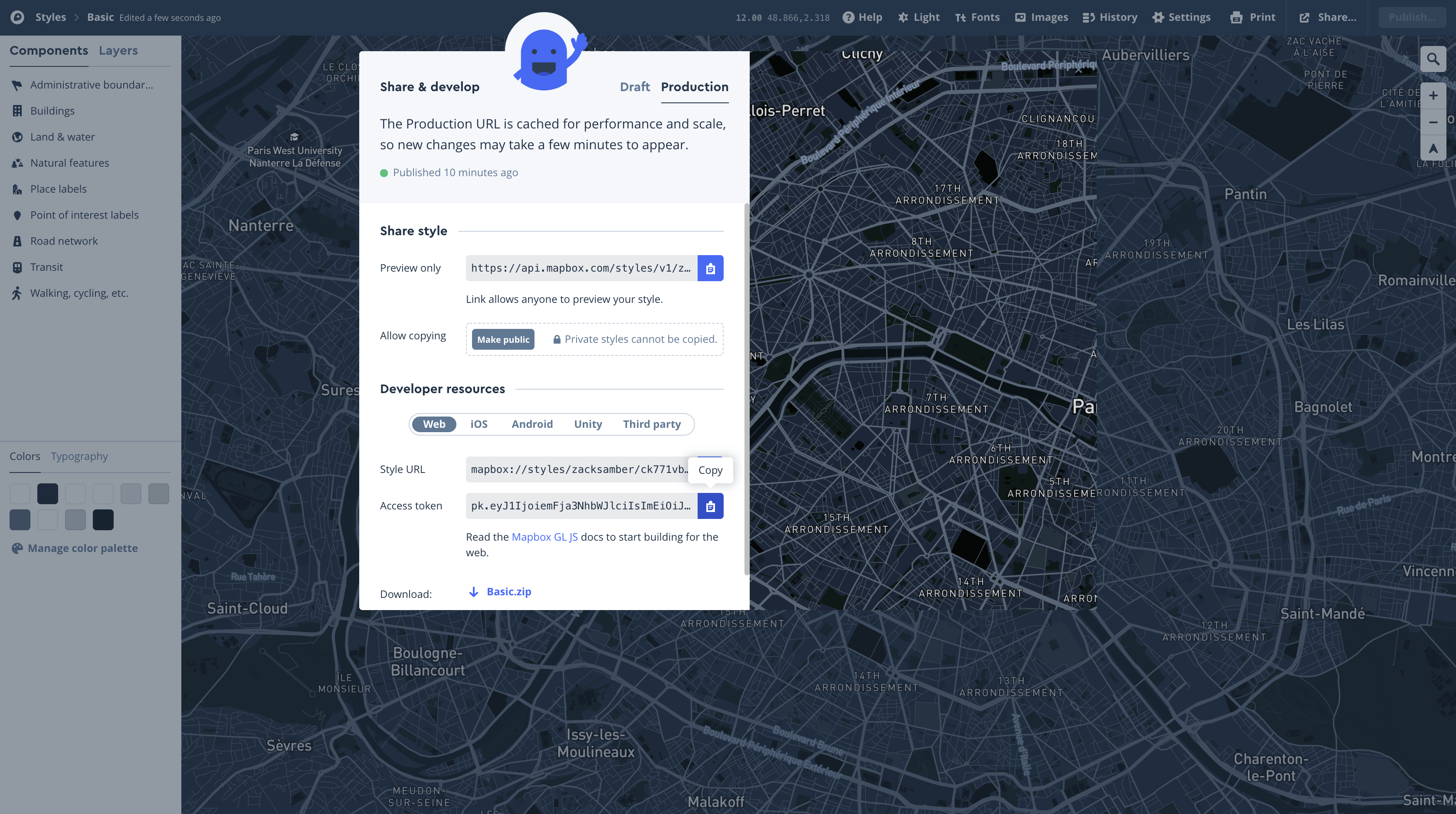
Then open your shell. Make sure you are in your .py file working directory.

CLI

pwd

ls -l

Then replace your Acess Token to the following command.

CLI

touch .mapbox_token
echo "Your Access Token" > .mapbox_token

---

Test Dataset px.carshare()

Python

# Test dataset px.data.carshare()
px.set_mapbox_access_token(open(".mapbox_token").read())
df = px.data.carshare()
fig = px.scatter_mapbox(df, 
                        lat='centroid_lat', 
                        lon='centroid_lon', 
                        color='peak_hour', 
                        size='car_hours', 
                        color_continuous_scale=px.colors.cyclical.IceFire, 
                        size_max=15, 
                        zoom=10)
fig.show()
# fig.write_image('fig.svg', scale=2)
# ![](https://raw.githubusercontent.com/ZacksAmber/PicGo/master/img/20210402000731.svg)

---

Back to dataset stations

mapbox_style (str (default 'basic', needs Mapbox API token)) – Identifier of base map style, some of which require a Mapbox API token to be set using plotly.express.set_mapbox_access_token(). Allowed values which do not require a Mapbox API token are 'open-street-map', 'white-bg', 'carto-positron', 'carto-darkmatter', 'stamen- terrain', 'stamen-toner', 'stamen-watercolor'. Allowed values which do require a Mapbox API token are 'basic', 'streets', 'outdoors', 'light', 'dark', 'satellite', 'satellite- streets'.

Python

# Draw map
# Test dataset px.data.carshare()

# Some mapbox_style do not require access token
# px.set_mapbox_access_token(open(".mapbox_token").read())
fig = px.scatter_mapbox(stations, 
                        lat='lat', 
                        lon='long', 
                        hover_name='name', 
                        center={'lat': 37.39028, 'lon': -122.0666}, 
                        mapbox_style='streets', 
                        size_max=15, 
                        zoom=10)
fig.show()
# fig.write_image('fig.svg', scale=2)
# ![](https://raw.githubusercontent.com/ZacksAmber/PicGo/master/img/20210402002931.svg)

The map is created using OpenStreetMap, which is an open online mapping system that you can use just as you would use Google Maps or any other online map. Zoom in to San Francisco to see how the stations are distributed. Click on a marker to see which station it is.

You can also represent points on a map by colored circles. Here is such a map of the San Francisco bike stations

Python

# Filter 'landmark' == 'San Francisco'
sf = stations[stations['landmark'] == 'San Francisco']
# Extract columns 'lat', 'long', 'name'
sf_map_data = sf.loc[:, ['lat', 'long', 'name']]

# Draw map
fig = px.scatter_mapbox(sf_map_data, 
                        lat='lat', 
                        lon='long', 
                        hover_name='name',  
                        mapbox_style='streets', 
                        size_max=15, 
                        zoom=12, 
                        color_discrete_sequence=['blue'])
fig.show()
# fig.write_image('fig.svg', scale=2)
# ![](https://raw.githubusercontent.com/ZacksAmber/PicGo/master/img/20210402002931.svg)

---

More Informative Maps: An Application of join

The bike stations are located in five different cities in the Bay Area. To distinguish the points by using a different color for each city, let’s start by using group to identify all the cities and assign each one a color.

Python

# SELECT landmark AS city, COUNT(*) AS 'count' FROM cities GROUP BY city;
cities = stations.groupby('landmark')['landmark'].count().reset_index(name='count').rename(columns={'landmark': 'city'})
cities

	city	count
0	Mountain View	7
1	Palo Alto	5
2	Redwood City	7
3	San Francisco	35
4	San Jose	16

Python

# Copy cities to colors then add a new columns
colors = cities.copy()
colors['color'] = np.array(['blue', 'red', 'green', 'orange', 'purple'])
colors

	city	count	color
0	Mountain View	7	blue
1	Palo Alto	5	red
2	Redwood City	7	green
3	San Francisco	35	orange
4	San Jose	16	purple

Now we can join stations and colors by landmark, and then select the columns we need to draw a map.

Python

# JOIN table stations and colors
joined = stations.join(colors.set_index('city'), 
                       on='landmark', 
                       how='inner')
colored = joined.loc[:, ['lat', 'long', 'name', 'color']]
colored

	lat	long	name	color
0	37.329732	-121.901782	San Jose Diridon Caltrain Station	purple
1	37.330698	-121.888979	San Jose Civic Center	purple
2	37.333988	-121.894902	Santa Clara at Almaden	purple
3	37.331415	-121.893200	Adobe on Almaden	purple
4	37.336721	-121.894074	San Pedro Square	purple
...	...	...	...	...
62	37.794139	-122.394434	Steuart at Market	orange
63	37.791300	-122.399051	Mechanics Plaza (Market at Battery)	orange
64	37.786305	-122.404966	Market at 4th	orange
65	37.789625	-122.400811	Market at Sansome	orange
67	37.798541	-122.400862	Broadway St at Battery St	orange

Python

# Draw map
fig = px.scatter_mapbox(colored, 
                        lat='lat', 
                        lon='long', 
                        hover_name='name',  
                        mapbox_style='streets', 
                        size_max=15, 
                        zoom=8, 
                        color='color', 
                        color_discrete_sequence=colored['color'].unique())
fig.show()
# fig.write_image('fig.svg', scale=2)
# ![](https://raw.githubusercontent.com/ZacksAmber/PicGo/master/img/20210402005612.svg)

Now the markers have five different colors for the five different cities.

To see where most of the bike rentals originate, let’s identify the start stations:

Python

 SELECT 'Start Station', COUNT(*) AS 'count' FROM commute GROUP BY 'Start Station' ORDER BY 'count' DESC;
starts = commute.groupby('Start Station')['Start Station'].count().reset_index(name='count').sort_values(by='count', ascending=False)
starts

	Start Station	count
49	San Francisco Caltrain (Townsend at 4th)	25858
50	San Francisco Caltrain 2 (330 Townsend)	21523
23	Harry Bridges Plaza (Ferry Building)	15543
65	Temporary Transbay Terminal (Howard at Beale)	14298
2	2nd at Townsend	13674
...	...	...
31	Mezes Park	189
41	Redwood City Medical Center	139
55	San Mateo County Center	108
42	Redwood City Public Library	101
20	Franklin at Maple	62

We can include the geographical data needed to map these stations, by first joining starts with stations:

Python

# INNER JOIN stations and starts
station_starts = stations.join(starts.set_index('Start Station'), 
                               on='name', 
                               how='inner')
station_starts

	station_id	name	lat	long	dockcount	landmark	installation	count
0	2	San Jose Diridon Caltrain Station	37.329732	-121.901782	27	San Jose	8/6/2013	4899
1	3	San Jose Civic Center	37.330698	-121.888979	15	San Jose	8/5/2013	574
2	4	Santa Clara at Almaden	37.333988	-121.894902	11	San Jose	8/6/2013	1888
3	5	Adobe on Almaden	37.331415	-121.893200	19	San Jose	8/5/2013	522
4	6	San Pedro Square	37.336721	-121.894074	15	San Jose	8/7/2013	1321
...	...	...	...	...	...	...	...	...
65	77	Market at Sansome	37.789625	-122.400811	27	San Francisco	8/25/2013	11023
66	80	Santa Clara County Civic Center	37.352601	-121.905733	15	San Jose	12/31/2013	510
67	82	Broadway St at Battery St	37.798541	-122.400862	15	San Francisco	1/22/2014	7460
68	83	Mezes Park	37.491269	-122.236234	15	Redwood City	2/20/2014	189
69	84	Ryland Park	37.342725	-121.895617	15	San Jose	4/9/2014	1077

Now we extract just the data needed for drawing our map, adding a color and an area to each station. The area is 0.3 times the count of the number of rentals starting at each station, where the constant 0.3 was chosen so that the circles would appear at an appropriate scale on the map.

Python

# Extract columns 'lat', 'long', 'name' from station_starts to starts_map_data
starts_map_data = station_starts.loc[:, ['lat', 'long', 'name']].copy()

# Set color
starts_map_data['colors'] = ['blue'] * 68 # 68 rows

# Set size
starts_map_data['areas'] = station_starts['count'] * 0.3

starts_map_data

	lat	long	name	colors	areas
0	37.329732	-121.901782	San Jose Diridon Caltrain Station	blue	1469.7
1	37.330698	-121.888979	San Jose Civic Center	blue	172.2
2	37.333988	-121.894902	Santa Clara at Almaden	blue	566.4
3	37.331415	-121.893200	Adobe on Almaden	blue	156.6
4	37.336721	-121.894074	San Pedro Square	blue	396.3
...	...	...	...	...	...
65	37.789625	-122.400811	Market at Sansome	blue	3306.9
66	37.352601	-121.905733	Santa Clara County Civic Center	blue	153.0
67	37.798541	-122.400862	Broadway St at Battery St	blue	2238.0
68	37.491269	-122.236234	Mezes Park	blue	56.7
69	37.342725	-121.895617	Ryland Park	blue	323.1

Python

# Draw map
fig = px.scatter_mapbox(starts_map_data, 
                        lat='lat', 
                        lon='long', 
                        hover_name='name',  
                        mapbox_style='streets', 
                        size='areas', 
                        size_max=15, 
                        center={'lat': 37.7766, 'lon': -122.3955}, 
                        zoom=10, 
                        color='colors',
                        color_discrete_sequence=starts_map_data['colors'].unique(), 
                        opacity=0.6)
fig.show()
# fig.write_image('fig.svg', scale=2)
# ![](https://raw.githubusercontent.com/ZacksAmber/PicGo/master/img/20210402011250.svg)

That huge blob in San Francisco shows that the eastern section of the city is the unrivaled capital of bike rentals in the Bay Area.

---

Randomness

Randomness
Program: Data8-9.ipynb

---

Randomness

In the previous chapters we developed skills needed to make insightful descriptions of data. Data scientists also have to be able to understand randomness. For example, they have to be able to assign individuals to treatment and control groups at random, and then try to say whether any observed differences in the outcomes of the two groups are simply due to the random assignment or genuinely due to the treatment.

In this chapter, we begin our analysis of randomness. To start off, we will use Python to make choices at random. In numpy there is a sub-module called random that contains many functions that involve random selection. One of these functions is called choice. It picks one item at random from an array, and it is equally likely to pick any of the items. The function call is np.random.choice(array_name), where array_name is the name of the array from which to make the choice.

Thus the following code evaluates to treatment with chance 50%, and control with chance 50%.

Python

# The following code evaluates to treatment with chance 50%, and control with chance 50%.
two_groups = np.array(['treatment', 'control'])
np.random.choice(two_groups)
# 'control'
# OR
# 'treatment'

The big difference between the code above and all the other code we have run thus far is that the code above doesn’t always return the same value. It can return either treatment or control, and we don’t know ahead of time which one it will pick. We can repeat the process by providing a second argument, the number of times to repeat the process.

Python

# Randomly choose 'treatment', 'control' from two_groups 10 times
np.random.choice(two_groups, 10)
'''
array(['treatment', 'treatment', 'treatment', 'treatment', 'treatment',
       'treatment', 'control', 'treatment', 'treatment', 'control'],
      dtype='<U9')
'''

A fundamental question about random events is whether or not they occur. For example:

• Did an individual get assigned to the treatment group, or not?
• Is a gambler going to win money, or not?
• Has a poll made an accurate prediction, or not?

Once the event has occurred, you can answer “yes” or “no” to all these questions. In programming, it is conventional to do this by labeling statements as True or False. For example, if an individual did get assigned to the treatment group, then the statement, “The individual was assigned to the treatment group” would be True. If not, it would be False.

---

Booleans and Comparison

In Python, Boolean values, named for the logician George Boole, represent truth and take only two possible values: True and False. Whether problems involve randomness or not, Boolean values most often arise from comparison operators. Python includes a variety of operators that compare values. For example, 3 is larger than 1 + 1.

Python

3 > 1 + 1
# True

The value True indicates that the comparison is valid; Python has confirmed this simple fact about the relationship between 3 and 1+1. The full set of common comparison operators are listed below.

Comparison	Operator	True example	False Example
Less than	<	2 < 3	2 < 2
Greater than	>	3 > 2	3 > 3
Less than or equal	<=	2 <= 2	3 <= 2
Greater or equal	>=	3 >= 3	2 >= 3
Equal	==	3 == 3	3 == 2
Not equal	!=	3 != 2	2 != 2

Notice the two equal signs == in the comparison to determine equality. This is necessary because Python already uses = to mean assignment to a name, as we have seen. It can’t use the same symbol for a different purpose. Thus if you want to check whether 5 is equal to the 10/2, then you have to be careful: 5 = 10/2 returns an error message because Python assumes you are trying to assign the value of the expression 10/2 to a name that is the numeral 5. Instead, you must use 5 == 10/2, which evaluates to True.

Python

5 = 10/2

Python

  File "<ipython-input-13-e8c755f5e450>", line 1
    5 = 10/2
    ^
SyntaxError: cannot assign to literal

An expression can contain multiple comparisons, and they all must hold in order for the whole expression to be True. For example, we can express that 1+1 is between 1 and 3 using the following expression.

Python

1 < 1 + 1 < 3
# True

The average of two numbers is always between the smaller number and the larger number. We express this relationship for the numbers x and y below. You can try different values of x and y to confirm this relationship.

Python

x = 12
y = 5
min(x, y) <= (x+y)/2 <= max(x, y)
# True

---

Comparing Strings

Strings can also be compared, and their order is alphabetical. A shorter string is less than a longer string that begins with the shorter string.

Python

'Dog' > 'Catastrophe' > 'Cat'
# True

Let’s return to random selection. Recall the array two_groups which consists of just two elements, treatment and control. To see whether a randomly assigned individual went to the treatment group, you can use a comparison:

Python

np.random.choice(two_groups) == 'treatment'

Python

True
# OR False

As before, the random choice will not always be the same, so the result of the comparison won’t always be the same either. It will depend on whether treatment or control was chosen. With any cell that involves random selection, it is a good idea to run the cell several times to get a sense of the variability in the result.

---

Comparing an Array and a Value

Recall that we can perform arithmetic operations on many numbers in an array at once. For example, np.array(0, 5, 2)*2 is equivalent to np.array(0, 10, 4). In similar fashion, if we compare an array and one value, each element of the array is compared to that value, and the comparison evaluates to an array of Booleans.

Python

tosses = np.array(['Tails', 'Heads', 'Tails', 'Heads', 'Heads'])
tosses == 'Heads'
# array([False,  True, False,  True,  True])

The numpy method count_nonzero evaluates to the number of non-zero (that is, True) elements of the array.

Python

np.count_nonzero(tosses == 'Heads')
# 3

---

Conditional Statements

In many situations, actions and results depends on a specific set of conditions being satisfied. For example, individuals in randomized controlled trials receive the treatment if they have been assigned to the treatment group. A gambler makes money if she wins her bet.

In this section we will learn how to describe such situations using code. A conditional statement is a multi-line statement that allows Python to choose among different alternatives based on the truth value of an expression. While conditional statements can appear anywhere, they appear most often within the body of a function in order to express alternative behavior depending on argument values.

A conditional statement always begins with an if header, which is a single line followed by an indented body. The body is only executed if the expression directly following if (called the if expression) evaluates to a true value. If the if expression evaluates to a false value, then the body of the if is skipped.

Let us start defining a function that returns the sign of a number.

Python

def sign(x):
    
    if x > 0:
        return 'Positive'

Python

sign(3)
# 'Positive'

This function returns the correct sign if the input is a positive number. But if the input is not a positive number, then the if expression evaluates to a false value, and so the return statement is skipped and the function call has no value.

Python

sign(-3)

So let us refine our function to return Negative if the input is a negative number. We can do this by adding an elif clause, where elif if Python’s shorthand for the phrase “else, if”.

Python

def sign(x):
    
    if x > 0:
        return 'Positive'
    
    elif x < 0:
        return 'Negative'

Now sign returns the correct answer when the input is -3:

Python

sign(-3)
# 'Negative'

What if the input is 0? To deal with this case, we can add another elif clause:

Python

def sign(x):
    
    if x > 0:
        return 'Positive'
    
    elif x < 0:
        return 'Negative'
    
    elif x == 0:
        return 'Neither positive nor negative'

Python

sign(0)
'Neither positive nor negative'

Equivalently, we can replace the final elif clause by an else clause, whose body will be executed only if all the previous comparisons are false; that is, if the input value is equal to 0.

Python

def sign(x):
    
    if x > 0:
        return 'Positive'
    
    elif x < 0:
        return 'Negative'
    
    else:
        return 'Neither positive nor negative'

Python

sign(0)
'Neither positive nor negative'

---

The General Form

A conditional statement can also have multiple clauses with multiple bodies, and only one of those bodies can ever be executed. The general format of a multi-clause conditional statement appears below.

Python

if <if expression>:
    <if body>
elif <elif expression 0>:
    <elif body 0>
elif <elif expression 1>:
    <elif body 1>
...
else:
    <else body>

There is always exactly one if clause, but there can be any number of elif clauses. Python will evaluate the if and elif expressions in the headers in order until one is found that is a true value, then execute the corresponding body. The else clause is optional. When an else header is provided, its else body is executed only if none of the header expressions of the previous clauses are true. The else clause must always come at the end (or not at all).

---

Example: Betting on a Die

Suppose I bet on a roll of a fair die. The rules of the game:

• If the die shows 1 spot or 2 spots, I lose a dollar.
• If the die shows 3 spots or 4 spots, I neither lose money nor gain money.
• If the die shows 5 spots or 6 spots, I gain a dollar.

We will now use conditional statements to define a function one_bet that takes the number of spots on the roll and returns my net gain.

Python

def one_bet(x):
    """Returns my net gain if the die shows x spots"""
    if x <= 2:
        return -1
    elif x <= 4:
        return 0
    elif x <= 6:
        return 1

Let’s check that the function does the right thing for each different number of spots.

Python

one_bet(1), one_bet(2), one_bet(3), one_bet (4), one_bet(5), one_bet(6)
# (-1, -1, 0, 0, 1, 1)

As a review of how conditional statements work, let’s see what one_bet does when the input is 3.

• First it evaluates the if expression, which is 3 <= 2 which is False. So one_bet doesn’t execute the if body.
• Then it evaluates the first elif expression, which is 3 <= 4, which is True. So one_bet executes the first elif body and returns 0.
• Once the body has been executed, the process is complete. The next elif expression is not evaluated.

If for some reason we use an input greater than 6, then the if expression evaluates to False as do both of the elif expressions. So one_bet does not execute the if body nor the two elif bodies, and there is no value when you make the call below.

Python

one_bet(17)

To play the game based on one roll of a die, you can use np.random.choice to generate the number of spots and then use that as the argument to one_bet. Run the cell a few times to see how the output changes.

Python

one_bet(np.random.choice(np.arange(1, 7)))
# 1

At this point it is natural to want to collect the results of all the bets so that we can analyze them. In the next section we develop a way to do this without running the cell over and over again.

---

Iteration

It is often the case in programming – especially when dealing with randomness – that we want to repeat a process multiple times. For example, recall the game of betting on one roll of a die with the following rules:

• If the die shows 1 or 2 spots, my net gain is -1 dollar.
• If the die shows 3 or 4 spots, my net gain is 0 dollars.
• If the die shows 5 or 6 spots, my net gain is 1 dollar.

The function bet_on_one_roll takes no argument. Each time it is called, it simulates one roll of a fair die and returns the net gain in dollars.

Python

def bet_on_one_roll():
    """Returns my net gain on one bet"""
    x = np.random.choice(np.arange(1, 7))  # roll a die once and record the number of spots
    if x <= 2:
        return -1
    elif x <= 4:
        return 0
    elif x <= 6:
        return 1

Playing this game once is easy:

Python

bet_on_one_roll()
# 1

To get a sense of how variable the results are, we have to play the game over and over again. We could run the cell repeatedly, but that’s tedious, and if we wanted to do it a thousand times or a million times, forget it.

A more automated solution is to use a for statement to loop over the contents of a sequence. This is called iteration. A for statement begins with the word for, followed by a name we want to give each item in the sequence, followed by the word in, and ending with an expression that evaluates to a sequence. The indented body of the for statement is executed once for each item in that sequence.

Python

for animal in np.array(['cat', 'dog', 'rabbit']):
    print(animal)
'''
cat
dog
rabbit
'''

It is helpful to write code that exactly replicates a for statement, without using the for statement. This is called unrolling the loop.

A for statement simple replicates the code inside it, but before each iteration, it assigns a new value from the given sequence to the name we chose. For example, here is an unrolled version of the loop above.

Python

animal = np.array(['cat', 'dog', 'rabbit']).item(0)
print(animal)
animal = np.array(['cat', 'dog', 'rabbit']).item(1)
print(animal)
animal = np.array(['cat', 'dog', 'rabbit']).item(2)
print(animal)
'''
cat
dog
rabbit
'''

Notice that the name animal is arbitrary, just like any name we assign with =.

Here we use a for statement in a more realistic way: we print the results of betting five times on the die as described earlier. This is called simulating the results of five bets. We use the word simulating to remind ourselves that we are not physically rolling dice and exchanging money but using Python to mimic the process.

To repeat a process n times, it is common to use the sequence np.arange(n) in the for statement. It is also common to use a very short name for each item. In our code we will use the name i to remind ourselves that it refers to an item.

Python

for i in np.arange(5):
    print(bet_on_one_roll())
'''
0
0
-1
-1
0
'''

In this case, we simply perform exactly the same (random) action several times, so the code in the body of our for statement does not actually refer to i.

---

Augmenting Arrays

While the for statement above does simulate the results of five bets, the results are simply printed and are not in a form that we can use for computation. Any array of results would be more useful. Thus a typical use of a for statement is to create an array of results, by augmenting the array each time.

The append method in NumPy helps us do this. The call np.append(array_name, value) evaluates to a new array that is array_name augmented by value. When you use append, keep in mind that all the entries of an array must have the same type.

Python

pets = np.array(['Cat', 'Dog'])
np.append(pets, 'Another Pet')
# array(['Cat', 'Dog', 'Another Pet'], dtype='<U11')

This keeps the array pets unchanged:

Python

pets
# array(['Cat', 'Dog'], dtype='<U3')

But often while using for loops it will be convenient to mutate an array – that is, change it – when augmenting it. This is done by assigning the augmented array to the same name as the original.

Python

pets = np.append(pets, 'Another Pet')
pets
# array(['Cat', 'Dog', 'Another Pet'], dtype='<U11')

---

Example: Betting on 5 Rolls

We can now simulate five bets on the die and collect the results in an array that we will call the collection array. We will start out by creating an empty array for this, and then append the outcome of each bet. Notice that the body of the for loop contains two statements. Both statements are executed for each item in the given sequence.

Python

# Make an empty array outcomes
outcomes = make_array()

# Betting on 5 rolls
for i in np.arange(5):
    outcome_of_bet = bet_on_one_roll()
    outcomes = np.append(outcomes, outcome_of_bet)
    
outcomes
# array([0., 1., 1., 0., 1.])

Let us rewrite the cell with the for statement unrolled:

Python

# Make an empty array outcomes
outcomes = np.array([])

# Betting on 5 rolls without using for loop
i = np.arange(5).item(0)
outcome_of_bet = bet_on_one_roll()
outcomes = np.append(outcomes, outcome_of_bet)

i = np.arange(5).item(1)
outcome_of_bet = bet_on_one_roll()
outcomes = np.append(outcomes, outcome_of_bet)

i = np.arange(5).item(2)
outcome_of_bet = bet_on_one_roll()
outcomes = np.append(outcomes, outcome_of_bet)

i = np.arange(5).item(3)
outcome_of_bet = bet_on_one_roll()
outcomes = np.append(outcomes, outcome_of_bet)

i = np.arange(5).item(4)
outcome_of_bet = bet_on_one_roll()
outcomes = np.append(outcomes, outcome_of_bet)

outcomes
# array([ 0., -1.,  1., -1.,  1.])

The contents of the array are likely to be different from the array that we got by running the previous cell, but that is because of randomness in rolling the die. The process for creating the array is exactly the same.

By capturing the results in an array we have given ourselves the ability to use array methods to do computations. For example, we can use np.count_nonzero to count the number of times money changed hands.

Python

np.count_nonzero(outcomes)
# 4

---

Example: Betting on 300 Rolls

Iteration is a powerful technique. For example, we can see the variation in the results of 300 bets by running exactly the same code for 300 bets instead of five.

Python

# Make an empty array outcomes
outcomes = np.array([])

# Betting on 300 rolls
for i in np.arange(300):
    outcome_of_bet = bet_on_one_roll()
    outcomes = np.append(outcomes, outcome_of_bet)

The array outcomes contains the results of all 300 bets.

Python

# Times of the rolling
len(outcomes)

To see how often the three different possible results appeared, we can use the array outcomes and px.bar methods.

plotly.express.bar

Python

# Save outcomes as DataFrame
outcome_table = pd.DataFrame({'Outcome': outcomes})

# SELECT Outcome, COUNT(*) AS 'count' FROM outcome_table GROUP BY Outcome;
outcome_table.groupby('Outcome')['Outcome'].count().reset_index(name='count')

	Outcome	count
0	-1.0	99
1	0.0	99
2	1.0	102

Python

# Draw bar chart
fig = px.bar(outcome_table.groupby('Outcome')['Outcome'].count().reset_index(name='count'), 
             x='count', 
             y='Outcome', 
             # 'h' for horizontal or 'v' for vertical
             orientation='h', 
             opacity=0.65, 
             color_discrete_sequence=['red'])
fig.show()
# fig.write_image('fig.svg', scale=2)
# ![](https://raw.githubusercontent.com/ZacksAmber/PicGo/master/img/20210402191004.svg)

Not surprisingly, each of the three outcomes -1, 0, and 1 appeared about 100 of the 300 times, give or take. We will examine the “give or take” amounts more closely in later chapters.

---

Simulation

Simulation is the process of using a computer to mimic a physical experiment. In this class, those experiments will almost invariably involve chance.

We have seen how to simulate the results of tosses of a coin. The steps in that simulation were examples of the steps that will constitute every simulation we do in this course. In this section we will set out those steps and follow them in examples.

---

Step 1: What to Simulate

Specify the quantity you want to simulate. For example, you might decide that you want to simulate the outcomes of tosses of a coin.

---

Step 2: Simulating One Value

Figure out how to simulate one value of the quantity you specified in Step 1. In our example, you have to figure out how to simulate the outcome of one toss of a coin. If your quantity is more complicated, you might need several lines of code to come up with one simulated value.

---

Step 3: Number of Repetitions

Decide how many times you want to simulate the quantity. You will have to repeat Step 2 that many times. In one of our earlier examples we had decided to simulate the outcomes of 1000 tosses of a coin, and so we needed 1000 repetitions of generating the outcome of a single toss.

---

Step 4: Coding the Simulation

Put it all together in code.

• Create an empty array in which to collect all the simulated values. We will call this the collection array.
• Create a “repetitions sequence,” that is, a sequence whose length is the number of repetitions you specified in Step 3. For n repetitions we will almost always use the sequence np.arange(n).
• Create a for loop. For each element of the repetitions sequence:
  • Simulate one value based on the code you developed in Step 2.
  • Augment the collection array with this simulated value.

That’s it! Once you have carried out the steps above, your simulation is done. The collection array contains all the simulated values.

At this point you can use the collection array as you would any other array. You can visualize the distribution of the simulated values, count how many simulated values fall into a particular category, and so on.

---

Number of Heads in 100 Tosses

It is natural to expect that in 100 tosses of a coin, there will be 50 heads, give or take a few.

But how many is “a few”? What’s the chance of getting exactly 50 heads? Questions like these matter in data science not only because they are about interesting aspects of randomness, but also because they can be used in analyzing experiments where assignments to treatment and control groups are decided by the toss of a coin.

In this example we will simulate the number of heads in 100 tosses of a coin. The histogram of our results will give us some insight into how many heads are likely.

Let’s get started on the simulation, following the steps above.

---

Step 1: What to Simulate

The quantity we are going to simulate is the number of heads in 100 tosses.

---

Step 2: Simulating One Value

We have to figure out how to make one set of 100 tosses and count the number of heads. Let’s start by creating a coin.

Python

# Define all possible values
coin = np.array(['Heads', 'Tails'])

In our earlier example we used np.random.choice and a for loop to generate multiple tosses. But sets of coin tosses are needed so often in data science that np.random.choice simulates them for us if we include a second argument that is the number of times to toss.

Here are the results of 10 tosses.

Python

# Toss the coin 10 times
ten_tosses = np.random.choice(coin, 10)
ten_tosses

Python

array(['Tails', 'Tails', 'Heads', 'Heads', 'Heads', 'Heads', 'Heads',
       'Heads', 'Heads', 'Tails'], dtype='<U5')

We can count the number of heads by using np.count_nonzero as before:

Python

# Count the number of Heads. Set 'Tails' as False(0), 'Head' as True(1)
np.count_nonzero(ten_tosses == 'Heads')

Our goal is to simulate the number of heads in 100 tosses, not 10. To do that we can just repeat the same code, replacing 10 by 100.

Python

# Toss the coin 100 times
outcomes = np.random.choice(coin, 100)
num_heads = np.count_nonzero(outcomes == 'Heads')
num_heads

Python

50

---

Step 3: Number of Repetitions

How many repetitions we want is up to us. The more we use, the more reliable our simulations will be, but the longer it will take to run the code. Python is pretty fast at tossing coins. Let’s go for 10,000 repetitions. That means we are going to do the following 10,000 times:

• Toss a coin 100 times and count the number of heads.

That’s a lot of tossing! It’s good that we have Python to do it for us.

---

Step 4: Coding the Simulation

We are ready to write the code to execute the entire simulation.

Python

# Tossing coin 100 times as one value. And repeat the process 10,000 times.
# An empty array to collect the simulated values
heads = np.array([])

# Repetitions sequence
num_repetitions = 10000
repetitions_sequence = np.arange(num_repetitions)

# for loop
for i in repetitions_sequence:
    # simulate one value
    outcomes = np.random.choice(coin, 100)
    num_heads = np.count_nonzero(outcomes == 'Heads')
    
    # augment the collection array with the simulated value
    heads = np.append(heads, num_heads)  

# That's it! The simulation is done.

Check that the array heads contains 10,000 entries, one for each repetition of the experiment.

Python

len(heads)
# 10000

To get a sense of the variability in the number of heads in 100 tosses, we can collect the results in a table and draw a histogram.

Python

# Make a DataFrame for storing the tossing result.
simulation_results = pd.DataFrame(
    {'Repetition': np.arange(1, num_repetitions + 1),
    'Number of Heads': heads}
)

simulation_results

	Repetition	Number of Heads
0	1	48.0
1	2	44.0
2	3	51.0
3	4	43.0
4	5	52.0
...	...	...
9995	9996	53.0
9996	9997	53.0
9997	9998	47.0
9998	9999	54.0
9999	10000	58.0

Python

# Draw histogram
fig = px.histogram(simulation_results, 
                   x='Number of Heads', 
                   histnorm='percent', 
                   opacity=0.7)
# Set bins
fig.update_traces(xbins=dict(start=30.5, end=69.6, size=1))

# Set layout
fig.update_layout(yaxis_title='Percent per unit')

fig.show()
# fig.write_image('fig.svg', scale=2)
# ![](https://raw.githubusercontent.com/ZacksAmber/PicGo/master/img/20210405162005.svg)

Each bin has width 1 and is centered at each value of the number of heads.

Not surprisingly, the histogram looks roughly symmetric around 50 heads. The height of the bar at 50 is about 8% per unit. Since each bin is 1 unit wide, this is the same as saying that about 8% of the repetitions produced exactly 50 heads. That’s not a huge percent, but it’s the largest compared to the percent at every other number of heads.

The histogram also shows that in almost all of the repetitions, the number of heads in 100 tosses was somewhere between 35 and 65. Indeed, the bulk of the repetitions produced numbers of heads in the range 45 to 55.

While in theory it is possible that the number of heads can be anywhere between 0 and 100, the simulation shows that the range of probable values is much smaller.

This is an instance of a more general phenomenon about the variability in coin tossing, as we will see later in the course.

---

A More Compact Version of the Code

We wrote the code for the simulation to show each of the steps in detail. Here are the same steps written in a more compact form. You can see that the code starts out the same way as before, but then some steps are combined.

Python

# Step 4: Create an empty array in which to collect all the simulated values. We will call this the collection array.
heads = np.array([])

# Create a “repetitions sequence,” that is, a sequence whose length is the number of repetitions you specified in Step 3. 
# For n repetitions we will almost always use the sequence np.arange(n).
num_repetitions = 10000

# Create a for loop. For each element of the repetitions sequence:
#  - Simulate one value based on the code you developed in Step 2.
#  - Augment the collection array with this simulated value.
for i in np.arange(num_repetitions):
    outcomes = np.random.choice(coin, 100)
    heads = np.append(heads, np.count_nonzero(outcomes == 'Heads'))

Python

# Show the results of 10,000 repetition
heads
# array([55., 48., 49., ..., 51., 48., 39.])

---

Moves in Monopoly

Each move in the game Monopoly is determined by the total number of spots of two rolls of a die. If you play Monopoly, what should you expect to get when you roll the die two times?

We can explore this by simulating the sum of two rolls of a die. We will run the simulation 10,000 times as we did in the previous example. Notice that in this paragraph we have completed Steps 1 and 3 of our simulation process.

Step 2 is the one in which we simulate one pair of rolls and add up the number of spots.

Python

# Define all possible values of one die
die = np.arange(1, 7)

# The result of two rolls of a die
sum(np.random.choice(die, 2))
# From 2 to 12

That simulates one value of the sum of two rolls. We are now all set to run the simulation according to the steps that are now familiar.

Python

# Step 4: Create an empty array in which to collect all the simulated values. We will call this the collection array.
moves = np.array([])

# Create a “repetitions sequence,” that is, a sequence whose length is the number of repetitions you specified in Step 3. 
# For n repetitions we will almost always use the sequence np.arange(n).
num_repetitions = 10000

# Create a for loop. For each element of the repetitions sequence:
#  - Simulate one value based on the code you developed in Step 2.
#  - Augment the collection array with this simulated value.
for i in np.arange(num_repetitions):
    one_move = sum(np.random.choice(die, 2))
    moves = np.append(moves, one_move)

Here is a histogram of the results.

Python

# Make a DataFrame for storing the rolling result.
results = pd.DataFrame(
    {'Repetition': np.arange(1, num_repetitions + 1),
    'Sum of Two Rolls': moves}
)

# Histogram
fig = px.histogram(results, 
                   x='Sum of Two Rolls', 
                   histnorm='percent', 
                   opacity=0.7, 
                   range_x = [1.5, 12.6], # np.arange(1.5, 12.6, 1)
                   nbins=12) # len(np.arange(1.5, 12.6, 1))

# Set bins
fig.update_traces(xbins=dict(start=1.5, end=12.6, size=1))

# Set layout
fig.update_layout(yaxis_title='Percent per unit')

fig.show()
# fig.write_image('fig.svg', scale=2)
# ![](https://raw.githubusercontent.com/ZacksAmber/PicGo/master/img/20210405162223.svg)

Seven is the most common value, with the frequencies falling off symmetrically on either side.

Becase P(sum of two rolls of a die): 6 * 6 = 36
When the sum is 7, it could be the following combinations:

• 1 + 6
• 2 + 5
• 3 + 4
• 4 + 3
• 5 + 2
• 6 + 1

P(sum = 7) = 6/36 = 1/6 = 16.7%

Python

len(results[results['Sum of Two Rolls']==7.0]) / len(results)
# 0.174

The percent of 'Sum of Two Rolls'=7 of simulation is close to the theoretical probability of P(sum=7).

---

The Monty Hall Problem

This problem has flummoxed many people over the years, mathematicians included. Let’s see if we can work it out by simulation.

The setting is derived from a television game show called “Let’s Make a Deal”. Monty Hall hosted this show in the 1960’s, and it has since led to a number of spin-offs. An exciting part of the show was that while the contestants had the chance to win great prizes, they might instead end up with “zonks” that were less desirable. This is the basis for what is now known as the Monty Hall problem.

The setting is a game show in which the contestant is faced with three closed doors. Behind one of the doors is a fancy car, and behind each of the other two there is a goat. The contestant doesn’t know where the car is, and has to attempt to find it under the following rules.

• The contestant makes an initial choice, but that door isn’t opened.
• At least one of the other two doors must have a goat behind it. Monty opens one of these doors to reveal a goat, displayed in all its glory in Wikipedia:

• There are two doors left, one of which was the contestant’s original choice. One of the doors has the car behind it, and the other one has a goat. The contestant now gets to choose which of the two doors to open.

The contestant has a decision to make. Which door should she choose to open, if she wants the car? Should she stick with her initial choice, or switch to the other door? That is the Monty Hall problem.

---

The Solution

In any problem involving chances, the assumptions about randomness are important. It’s reasonable to assume that there is a 1/3 chance that the contestant’s initial choice is the door that has the car behind it.

The solution to the problem is quite straightforward under this assumption, though the straightforward solution doesn’t convince everyone. Here it is anyway.

• The chance that the car is behind the originally chosen door is 1/3.
• The car is behind either the originally chosen door or the door that remains. It can’t be anywhere else.
• Therefore, the chance that the car is behind the door that remains is 2/3.
• Therefore, the contestant should switch.

That’s it. End of story.

Not convinced? Then let’s simulate the game and see how the results turn out.

---

Simulation

The simulation will be more complex that those we have done so far. Let’s break it down.

---

Step 1: What to Simulate

For each play we will simulate what’s behind all three doors:

• the one the contestant first picks
• the one that Monty opens
• the remaining door

So we will be keeping track of three quantities, not just one.

---

Step 2: Simulating One Play

The bulk of our work consists of simulating one play of the game. This involves several pieces.

---

The Goats

We start by setting up an array goats that contains unimaginative names for the two goats.

Python

# Define goats
goats = np.array(['first goat', 'second goat'])

To help Monty conduct the game, we are going to have to identify which goat is selected and which one is revealed behind the open door. The function other_goat takes one goat and returns the other.

Python

# Define goat remain
def other_goat(x):
    if x == 'first goat':
        return 'second goat'
    elif x == 'second goat':
        return 'first goat'

Let’s confirm that the function works.

Python

other_goat('first goat'), other_goat('second goat'), other_goat('watermelon')
# ('second goat', 'first goat', None)

The string ‘watermelon’ is not the name of one of the goats, so when ‘watermelon’ is the input then other_goat does nothing.

---

The Options

The array hidden_behind_doors contains the set of things that could be behind the doors.

Python

# Define all possbile options.
hidden_behind_doors = np.array(['car', 'first goat', 'second goat'])

We are now ready to simulate one play. To do this, we will define a function monty_hall_game that takes no arguments. When the function is called, it plays Monty’s game once and returns a list consisting of:

• the contestant’s guess
• what Monty reveals when he opens a door
• what remains behind the other door

The game starts with the contestant choosing one door at random. In doing so, the contestant makes a random choice from among the car, the first goat, and the second goat.

If the contestant happens to pick one of the goats, then the other goat is revealed and the car is behind the remaining door.

If the contestant happens to pick the car, then Monty reveals one of the goats and the other goat is behind the remaining door.

Python

# Define Monty Hall Game
def monty_hall_game():
    """Return 
    [contestant's guess, what Monty reveals, what remains behind the other door]"""
    
    contestant_guess = np.random.choice(hidden_behind_doors)
    
    if contestant_guess == 'first goat':
        return [contestant_guess, 'second goat', 'car']
    
    if contestant_guess == 'second goat':
        return [contestant_guess, 'first goat', 'car']
    
    if contestant_guess == 'car':
        revealed = np.random.choice(goats)
        return [contestant_guess, revealed, other_goat(revealed)]

Let’s play! Run the cell several times and see how the results change.

Python

monty_hall_game()
# ['second goat', 'first goat', 'car']

---

Step 3: Number of Repetitions

To gauge the frequency with which the different results occur, we have to play the game many times and collect the results. Let’s run 10,000 repetitions.

---

Step 4: Coding the Simulation

It’s time to run the whole simulation.

We will play the game 10,000 times and collect the results in a table. Each row of the table will contain the result of one play.

One way to grow a table by adding a new row is to use the append method. If df is a DataFrame and new_row is a list containing the entries in a new row, then df.loc[len(df)] = new_row adds the new row to the bottom of df. To add/replace new_row to specific location, run df.loc[<row_num>] = new_row.

Note that append does not create a new table. It changes df to have one more row than it did before.

First let’s create a table games that has three empty columns. We can do this by just specifying a list of the column labels, as follows.

Python

# Define DataFrame games for storing the game restults
games = pd.DataFrame(columns=['Guess', 'Revealed', 'Remaining'])

Notice that we have chosen the order of the columns to be the same as the order in which monty_hall_game returns the result of one game.

Now we can add 10,000 rows to trials. Each row will represent the result of one play of Monty’s game.

Python

# Play the game 10000 times and record the results in the table games

for i in np.arange(10000):
    games.loc[i] = monty_hall_game()

Python

games

	Guess	Revealed	Remaining
0	car	first goat	second goat
1	second goat	first goat	car
2	car	first goat	second goat
3	car	second goat	first goat
4	second goat	first goat	car
...	...	...	...
9995	second goat	first goat	car
9996	first goat	second goat	car
9997	second goat	first goat	car
9998	first goat	second goat	car
9999	first goat	second goat	car

The simulation is done. Notice how short the code is. The majority of the work was done in simulating the outcome of one game.

---

Visualization

To see whether the contestant should stick with her original choice or switch, let’s see how frequently the car is behind each of her two options.

Python

# SELECT 'Guess', COUNT(*) AS 'Original Door' FROM original_choice GROUP BY 'Guess';
original_choice = games.groupby('Guess')['Guess'].count().reset_index(name='Original Door')

# Rename column Guess to Item
original_choice.rename(columns={'Guess': 'Item'}, inplace=True)
original_choice

	Item	Original Door
0	car	3276
1	first goat	3307
2	second goat	3417

Python

# SELECT 'Remaining', COUNT(*) AS 'Redmaining Door' FROM original_choice GROUP BY 'Remaining';
remaining_door = games.groupby('Remaining')['Remaining'].count().reset_index(name='Redmaining Door')

# Rename column Remaining to Item
remaining_door.rename(columns={'Remaining': 'Item'}, inplace=True)
remaining_door

	Item	Redmaining Door
0	car	6724
1	first goat	1607
2	second goat	1669

As our earlier solution said, the car is behind the remaining door two-thirds of the time, to a pretty good approximation. The contestant is twice as likely to get the car if she switches than if she sticks with her original choice.

To see this graphically, we can join the two tables above and draw overlaid bar charts.

Python

# SELECT o.Item, o.'Original Door', r.'Redmaining Door' FROM original_choice o INNER JOIN remaining_door r USING(Item); 
joined = original_choice.join(remaining_door.set_index('Item'), on='Item', how='inner')
joined

	Item	Original Door	Redmaining Door
0	car	3276	6724
1	first goat	3307	1607
2	second goat	3417	1669

Python

# Bar chart
fig = px.bar(joined, 
             x=['Redmaining Door', 'Original Door'], 
             y='Item', 
             barmode='group', 
             category_orders={'Item': ['car', 'first goat', 'second goat']}, 
             color_discrete_sequence=['gold', 'blue'], 
             opacity=0.65)
fig.show()
# fig.write_image('fig.svg', scale=2)
# ![](https://raw.githubusercontent.com/ZacksAmber/PicGo/master/img/20210403222317.svg)

Notice how the three blue bars are almost equal – the original choice is equally likely to be any of the three available items. But the gold bar corresponding to Car is twice as long as the blue.

The simulation confirms that the contestant is twice as likely to win if she switches.

---

Finding Probabilities

Over the centuries, there has been considerable philosophical debate about what probabilities are. Some people think that probabilities are relative frequencies; others think they are long run relative frequencies; still others think that probabilities are a subjective measure of their own personal degree of uncertainty.

In this course, most probabilities will be relative frequencies, though many will have subjective interpretations. Regardless, the ways in which probabilities are calculated and combined are consistent across the different interpretations.

By convention, probabilities are numbers between 0 and 1, or, equivalently, 0% and 100%. Impossible events have probability 0. Events that are certain have probability 1.

Math is the main tool for finding probabilities exactly, though computers are useful for this purpose too. Simulation can provide excellent approximations, with high probability. In this section, we will informally develop a few simple rules that govern the calculation of probabilities. In subsequent sections we will return to simulations to approximate probabilities of complex events.

We will use the standard notation $P(event)$ to denote the probability that “event” happens, and we will use the words “chance” and “probability” interchangeably.

---

When an Event Doesn’t Happen

If the chance that event happens is 40%, then the chance that it doesn’t happen is 60%. This natural calculation can be described in general as follows:

$$P(\mbox{an event doesn’t happen}) = 1 - P(\mbox{the event happens})$$

---

When All Outcomes are Equally Likely

If you are rolling an ordinary die, a natural assumption is that all six faces are equally likely. Then probabilities of how one roll comes out can be easily calculated as a ratio. For example, the chance that the die shows an even number is

$$\frac{\mbox{number of even faces}}{\mbox{number of all faces}} = \frac{\mbox{ #{ 2, 4, 6 } }}{\mbox{ #{ 1, 2, 3, 4, 5, 6 } }} = \frac{3}{6}$$

Similarly,

$$P(\mbox{die shows a multiple of 3}) = \frac{\mbox{ #{ 3, 6 } }}{\mbox{ #{ 1, 2, 3, 4, 5, 6 } }} = \frac{2}{6}$$

In general,

$$P(\mbox{an event happens}) = \frac{\mbox{ #{ outcomes that make the event happen } }}{\mbox{ #{ all outcomes } }}$$

provided all the outcomes are equally likely.

Not all random phenomena are as simple as one roll of a die. The two main rules of probability, developed below, allow mathematicians to find probabilities even in complex situations.

---

When Two Events Must Both Happen

Suppose you have a box that contains three tickets: one red, one blue, and one green. Suppose you draw two tickets at random without replacement; that is, you shuffle the three tickets, draw one, shuffle the remaining two, and draw another from those two. What is the chance you get the green ticket first, followed by the red one?

There are six possible pairs of colors: RB, BR, RG, GR, BG, GB (we’ve abbreviated the names of each color to just its first letter). All of these are equally likely by the sampling scheme, and only one of them (GR) makes the event happen. So

$$P(\mbox{green first, then red}) = \frac{\mbox{ #{ GR } }}{\mbox{ #{ RB, BR, RG, GR, BG, GB } }} = \frac{1}{6}$$

But there is another way of arriving at the answer, by thinking about the event in two stages. First, the green ticket has to be drawn. That has chance 1/3, which means that the green ticket is drawn first in about 1/3 of all repetitions of the experiment. But that doesn’t complete the event. Among the 1/3 of repetitions when green is drawn first, the red ticket has to be drawn next. That happens in about 1/2 of those repetitions, and so:

$$P(\mbox{green first, then red}) = \frac{1}{2} \space \mbox{of} \space \frac{1}{3} = \frac{1}{6}$$

This calculation is usually written “in chronological order,” as follows.

$$P(\mbox{green first, then red}) = \frac{1}{3} \times \frac{1}{2} = \frac{1}{6}$$

The factor of 1/2 is called ” the conditional chance that the red ticket appears second, given that the green ticket appeared first.”

In general, we have the multiplication rule:

$$P\mbox{(two events both happen)} = P\mbox{(one event happens)} \times P\mbox{(the other event happens, given that the first one happened)}$$

Thus, when there are two conditions – one event must happen, as well as another – the chance is a fraction of a fraction, which is smaller than either of the two component fractions. The more conditions that have to be satisfied, the less likely they are to all be satisfied.

---

When an Event Can Happen in Two Different Ways

Suppose instead we want the chance that one of the two tickets is green and the other red. This event doesn’t specify the order in which the colors must appear. So they can appear in either order.

A good way to tackle problems like this is to partition the event so that it can happen in exactly one of several different ways. The natural partition of “one green and one red” is: GR, RG.

Each of GR and RG has chance 1/6 by the calculation above. So you can calculate the chance of “one green and one red” by adding them up.

$$P(\mbox{one green and one red}) = P(\mbox{GR}) + P(\mbox{RG}) =
\frac{1}{6} + \frac{1}{6} = \frac{2}{6}$$

In general, we have the addition rule:

$$P\mbox{(an event happens)} = P\mbox{(first way it can happen)} + P\mbox{(second way it can happen)}$$

provided the event happens in exactly one of the two ways.

Thus, when an event can happen in one of two different ways, the chance that it happens is a sum of chances, and hence bigger than the chance of either of the individual ways.

The multiplication rule has a natural extension to more than two events, as we will see below. So also the addition rule has a natural extension to events that can happen in one of several different ways.

We end the section with examples that use combinations of all these rules.

---

At Least One Success

Data scientists often work with random samples from populations. A question that sometimes arises is about the likelihood that a particular individual in the population is selected to be in the sample. To work out the chance, that individual is called a “success,” and the problem is to find the chance that the sample contains a success.

To see how such chances might be calculated, we start with a simpler setting: tossing a coin two times.

If you toss a coin twice, there are four equally likely outcomes: HH, HT, TH, and TT. We have abbreviated “Heads” to H and “Tails” to T. The chance of getting at least one head in two tosses is therefore 3/4.

Another way of coming up with this answer is to work out what happens if you don’t get at least one head: both the tosses have to land tails. So

$$P(\mbox{at least one head in two tosses}) = 1 - P(\mbox{both tails}) = 1 - \frac{1}{4} = \frac{3}{4}$$

Notice also that

$$P(\mbox{both tails}) = \frac{1}{4} = \frac{1}{2} \cdot \frac{1}{2} = \left(\frac{1}{2}\right)^2$$

by the multiplication rule.

These two observations allow us to find the chance of at least one head in any given number of tosses. For example,

$$P(\mbox{at least one head in 17 tosses}) = 1 - P(\mbox{all 17 are tails}) = 1 - \left(\frac{1}{2}\right)^{17}$$

And now we are in a position to find the chance that the face with six spots comes up at least once in rolls of a die.

For example,

$$P(\mbox{a single roll is not 6}) = P(1) + P(2) + P(3) + P(4) + P(5)
= \frac{5}{6}$$

Therefore,

$$P(\mbox{at least one 6 in two rolls}) = 1 - P(\mbox{both rolls are not 6}) = 1 - \left(\frac{5}{6}\right)^2$$

and

$$P(\mbox{at least one 6 in 17 rolls}) = 1 - \left(\frac{5}{6}\right)^{17}$$

The table below shows these probabilities as the number of rolls increases from 1 to 50.

Python

# Define rolls
rolls = np.arange(1, 51, 1)

# Define DataFrame results for storing roll results
results = pd.DataFrame({'Rolls': rolls, 
                        'Chance of at least one 6': 1 - (5/6)**rolls})
results

	Rolls	Chance of at least one 6
0	1	0.166667
1	2	0.305556
2	3	0.421296
3	4	0.517747
4	5	0.598122
...	...	...
45	46	0.999772
46	47	0.999810
47	48	0.999842
48	49	0.999868
49	50	0.999890

The chance that a 6 appears at least once rises rapidly as the number of rolls increases.

Python

# Draw scatter plot
fig = px.scatter(results, x='Rolls', y='Chance of at least one 6')
fig.show()
# fig.write_image('fig.svg', scale=2)
# ![](https://raw.githubusercontent.com/ZacksAmber/PicGo/master/img/20210403234128.svg)

In 50 rolls, you are almost certain to get at least one 6.

Python

# SELECT * FROM results where Rolls=50;
results[results.Rolls == 50]

	Rolls	Chance of at least one 6
49	50	0.99989

Calculations like these can be used to find the chance that a particular individual is selected in a random sample. The exact calculation will depend on the sampling scheme. But what we have observed above can usually be generalized: increasing the size of the random sample increases the chance that an individual is selected.

---

Sampling and Empirical Distributions

Sampling and Empirical Distributions
Program: Data8-10.ipynb

---

Sampling and Empirical Distributions

An important part of data science consists of making conclusions based on the data in random samples. In order to correctly interpret their results, data scientists have to first understand exactly what random samples are.

In this chapter we will take a more careful look at sampling, with special attention to the properties of large random samples.

Let’s start by drawing some samples. Our examples are based on the top_movies.csv data set.

Python

# Import dataset top_movies
top = pd.read_csv('https://raw.githubusercontent.com/ZacksAmber/Code/master/Data%20Science/Data8/Data%20Sets/top_movies.csv')

	Title	Studio	Gross	Gross (Adjusted)	Year
0	Star Wars: The Force Awakens	Buena Vista (Disney)	906723418	906723400	2015
1	Avatar	Fox	760507625	846120800	2009
2	Titanic	Paramount	658672302	1178627900	1997
3	Jurassic World	Universal	652270625	687728000	2015
4	Marvel's The Avengers	Buena Vista (Disney)	623357910	668866600	2012
...	...	...	...	...	...
195	The Caine Mutiny	Columbia	21750000	386173500	1954
196	The Bells of St. Mary's	RKO	21333333	545882400	1945
197	Duel in the Sun	Selz.	20408163	443877500	1946
198	Sergeant York	Warner Bros.	16361885	418671800	1941
199	The Four Horsemen of the Apocalypse	MPC	9183673	399489800	1921

---

Sampling Rows of a Table

Each row of a data table represents an individual; in top, each individual is a movie. Sampling individuals can thus be achieved by sampling the rows of a table.

The contents of a row are the values of different variables measured on the same individual. So the contents of the sampled rows form samples of values of each of the variables.

---

Deterministic Samples

When you simply specify which elements of a set you want to choose, without any chances involved, you create a deterministic sample.

You have done this many times, for example by using take:

You have done this many times, for example by using Pandas DataFrame.iloc:

pandas.DataFrame.iloc

Python

# Deterministic Sample
top.iloc[[3, 18, 100], :]

	Title	Studio	Gross	Gross (Adjusted)	Year
3	Jurassic World	Universal	652270625	687728000	2015
18	Spider-Man	Sony	403706375	604517300	2002
100	Gone with the Wind	MGM	198676459	1757788200	1939

You have also used Pandas Series.str.contains:

pandas.Series.str.contains

Python

# Deterministic Sample
top.loc[top.Title.str.contains('Harry Potter', regex=False)]
# OR
# top[top.Title.str.contains('Harry Potter', regex=False)]

	Title	Studio	Gross	Gross (Adjusted)	Year
22	Harry Potter and the Deathly Hallows Part 2	Warner Bros.	381011219	417512200	2011
43	Harry Potter and the Sorcerer's Stone	Warner Bros.	317575550	486442900	2001
54	Harry Potter and the Half-Blood Prince	Warner Bros.	301959197	352098800	2009
59	Harry Potter and the Order of the Phoenix	Warner Bros.	292004738	369250200	2007
62	Harry Potter and the Goblet of Fire	Warner Bros.	290013036	393024800	2005
69	Harry Potter and the Chamber of Secrets	Warner Bros.	261988482	390768100	2002
76	Harry Potter and the Prisoner of Azkaban	Warner Bros.	249541069	349598600	2004

While these are samples, they are not random samples. They don’t involve chance.

---

Probability Samples

For describing random samples, some terminology will be helpful.

A population is the set of all elements from whom a sample will be drawn.

A probability sample is one for which it is possible to calculate, before the sample is drawn, the chance with which any subset of elements will enter the sample.

In a probability sample, all elements need not have the same chance of being chosen.

---

A Random Sampling Scheme

For example, suppose you choose two people from a population that consists of three people A, B, and C, according to the following scheme:

• Person A is chosen with probability 1.
• One of Persons B or C is chosen according to the toss of a coin: if the coin lands heads, you choose B, and if it lands tails you choose C.

This is a probability sample of size 2. Here are the chances of entry for all non-empty subsets:

A: 1 
B: 1/2
C: 1/2
AB: 1/2
AC: 1/2
BC: 0
ABC: 0

Person A has a higher chance of being selected than Persons B or C; indeed, Person A is certain to be selected. Since these differences are known and quantified, they can be taken into account when working with the sample.

---

A Systematic Sample

Imagine all the elements of the population listed in a sequence. One method of sampling starts by choosing a random position early in the list, and then evenly spaced positions after that. The sample consists of the elements in those positions. Such a sample is called a systematic sample.

Here we will choose a systematic sample of the rows of top. We will start by picking one of the first 10 rows at random, and then we will pick every 10th row after that.

Python

"""Choose a random start among rows 0 through 9;
then take every 10th row."""

start = np.random.choice(np.arange(10))
top.iloc[np.arange(start, len(top), 10), :]

	Title	Studio	Gross	Gross (Adjusted)	Year
4	Marvel's The Avengers	Buena Vista (Disney)	623357910	668866600	2012
14	The Lion King	Buena Vista (Disney)	422783777	775573900	1994
24	Star Wars: Episode III - Revenge of the Sith	Fox	380270577	516123900	2005
34	The Hunger Games: Mockingjay - Part 1	Lionsgate	337135885	354324000	2014
44	Indiana Jones and the Kingdom of the Crystal S...	Paramount	317101119	384231200	2008
54	Harry Potter and the Half-Blood Prince	Warner Bros.	301959197	352098800	2009
64	Home Alone	Fox	285761243	589287500	1990
74	Night at the Museum	Fox	250863268	322261900	2006
84	Beverly Hills Cop	Paramount	234760478	584205200	1984
94	Saving Private Ryan	Dreamworks	216540909	397999500	1998
104	Snow White and the Seven Dreamworksarfs	Disney	184925486	948300000	1937
114	There's Something About Mary	Fox	176484651	326064000	1998
124	The Firm	Paramount	158348367	332761100	1993
134	National Lampoon's Animal House	Universal	141600000	521045300	1978
144	The Towering Inferno	Fox	116000000	533968300	1974
154	9 to 5	Fox	103290500	334062200	1980
164	Young Frankenstein	Fox	86273333	397131200	1974
174	The Ten Commandments	Paramount	65500000	1139700000	1956
184	Lawrence of Arabia	Columbia	44824144	481836900	1962
194	The Best Years of Our Lives	RKO	23650000	478500000	1946

Run the cell a few times to see how the output varies.

This systematic sample is a probability sample. In this scheme, all rows have chance 1/10 of being chosen. For example, Row 23 is chosen if and only if Row 3 is chosen, and the chance of that is 1/10.

But not all subsets have the same chance of being chosen. Because the selected rows are evenly spaced, most subsets of rows have no chance of being chosen. The only subsets that are possible are those that consist of rows all separated by multiples of 10. Any of those subsets is selected with chance 1/10. Other subsets, like the subset containing the first 11 rows of the table, are selected with chance 0.

---

Random Samples Drawn With or Without Replacement

In this course, we will mostly deal with the two most straightforward methods of sampling.

The first is random sampling with replacement, which (as we have seen earlier) is the default behavior of np.random.choice when it samples from an array.

The other, called a “simple random sample”, is a sample drawn at random without replacement. Sampled individuals are not replaced in the population before the next individual is drawn. This is the kind of sampling that happens when you deal a hand from a deck of cards, for example.

In this chapter, we will use simulation to study the behavior of large samples drawn at random with or without replacement.

Drawing a random sample requires care and precision. It is not haphazard, even though that is a colloquial meaning of the word “random”. If you stand at a street corner and take as your sample the first ten people who pass by, you might think you’re sampling at random because you didn’t choose who walked by. But it’s not a random sample – it’s a sample of convenience. You didn’t know ahead of time the probability of each person entering the sample; perhaps you hadn’t even specified exactly who was in the population.

---

Empirical Distributions

In data science, the word “empirical” means “observed”. Empirical distributions are distributions of observed data, such as data in random samples.

In this section we will generate data and see what the empirical distribution looks like.

Our setting is a simple experiment: rolling a die multiple times and keeping track of which face appears. The table die contains the numbers of spots on the faces of a die. All the numbers appear exactly once, as we are assuming that the die is fair.

---

Python

# Define all possible results
die = pd.DataFrame({'Face': np.arange(1, 7, 1)})
die

	Face
0	1
1	2
2	3
3	4
4	5
5	6

---

A Probability Distribution

The histogram below helps us visualize the fact that every face appears with probability 1/6. We say that the histogram shows the distribution of probabilities over all the possible faces. Since all the bars represent the same percent chance, the distribution is called uniform on the integers 1 through 6.

Python

# Histogram
fig = px.histogram(die, 
                   histnorm='percent', 
                   x='Face', 
                   opacity=0.7)

# Set bins
fig.update_traces(xbins=dict(start=0.5, end=6.6, size=1))

# Set layout
fig.update_layout(yaxis_title='Percent per unit')

fig.show()
# fig.write_image('fig.svg', scale=2)
# ![](https://raw.githubusercontent.com/ZacksAmber/PicGo/master/img/20210405162646.svg)

Variables whose successive values are separated by the same fixed amount, such as the values on rolls of a die (successive values separated by 1), fall into a class of variables that are called discrete. The histogram above is called a discrete histogram. Its bins are specified by the array die_bins and ensure that each bar is centered over the corresponding integer value.

It is important to remember that the die can’t show 1.3 spots, or 5.2 spots – it always shows an integer number of spots. But our visualization spreads the probability of each value over the area of a bar. While this might seem a bit arbitrary at this stage of the course, it will become important later when we overlay smooth curves over discrete histograms.

Before going further, let’s make sure that the numbers on the axes make sense. The probability of each face is 1/6, which is 16.67% when rounded to two decimal places. The width of each bin is 1 unit. So the height of each bar is 16.67% per unit. This agrees with the horizontal and vertical scales of the graph.

---

Empirical Distributions

The distribution above consists of the theoretical probability of each face. It is not based on data. It can be studied and understood without any dice being rolled.

Empirical distributions, on the other hand, are distributions of observed data. They can be visualized by empirical histograms.

Let us get some data by simulating rolls of a die. This can be done by sampling at random with replacement from the integers 1 through 6. We have used np.random.choice for such simulations before. But now we will introduce a Pandas method for doing this.

The Pandas method is called sample. It draws at random with replacement from the rows of a table. Its argument is the sample size, and it returns a table consisting of the rows that were selected. An optional argument with_replacement=False specifies that the sample should be drawn without replacement, but that does not apply to rolling a die.

Here are the results of 10 rolls of a die.

numpy.random.choice
Stop using numpy.random.seed()
NEP 19 — Random Number Generator Policy

Python

# Numpy np.random.choice
rng = np.random.default_rng(2021)
rng.choice(die.Face, 10, replace=True)
# array([5, 5, 3, 6, 4, 4, 4, 2, 4, 4])

pandas.DataFrame.sample
pandas.Series.sample
pandas.core.groupby.DataFrameGroupBy.sample

Python

# Pandas pd.DataFrame.sample
die.sample(n=10, replace=True, random_state=2021)

	Face
4	5
5	6
1	2
0	1
5	6
4	5
3	4
5	6
5	6
5	6

We can use the same method to simulate as many rolls as we like, and then draw empirical histograms of the results. Because we are going to do this repeatedly, we define a function empirical_hist_die that takes the sample size as its argument, rolls a die as many times as its argument, and then draws a histogram of the observed results.

Python

# Define Empirical Histogram Function
def empirical_hist_die(n):
    # Run one experiment
    die_sample = die.sample(n=n, replace=True, random_state=2021)
    # Define Empirical Histogram
    fig = px.histogram(die_sample, 
                       histnorm='percent', 
                       x='Face', 
                       opacity=0.65)
    # Set bins
    fig.update_traces(xbins=dict(start=0.5, end=6.6, size=1))
    # Set layout
    fig.update_layout(title='Sample Size = ' + str(n), 
                      yaxis_title='Percent per unit')
    
    fig.show()
    fig.write_image('fig.svg', scale=2)

---

Empirical Histograms

Here is an empirical histogram of 10 rolls. It doesn’t look very much like the probability histogram above. Run the cell a few times to see how it varies.

Python

# Call function, sample size=10
empirical_hist_die(10)

When the sample size increases, the empirical histogram begins to look more like the histogram of theoretical probabilities.

Python

# Call function, sample size=100
empirical_hist_die(100)

Python

# Call function, sample size=1000
empirical_hist_die(1000)

---

The Law of Averages

What we have observed above is an instance of a general rule.

If a chance experiment is repeated independently and under identical conditions, then, in the long run, the proportion of times that an event occurs gets closer and closer to the theoretical probability of the event.

For example, in the long run, the proportion of times the face with four spots appears gets closer and closer to 1/6.

Here “independently and under identical conditions” means that every repetition is performed in the same way regardless of the results of all the other repetitions.

---

Sampling from a Population

The law of averages also holds when the random sample is drawn from individuals in a large population.

As an example, we will study a population of flight delay times. The table united contains data for United Airlines domestic flights departing from San Francisco in the summer of 2015. The data are made publicly available by the Bureau of Transportation Statistics in the United States Department of Transportation.

There are 13,825 rows, each corresponding to a flight. The columns are the date of the flight, the flight number, the destination airport code, and the departure delay time in minutes. Some delay times are negative; those flights left early.

Python

# Import dataset united_summer2015.csv
united = pd.read_csv('https://github.com/ZacksAmber/Code/raw/master/Data%20Science/Data8/Data%20Sets/united_summer2015.csv')
united

	Date	Flight Number	Destination	Delay
0	6/1/15	73	HNL	257
1	6/1/15	217	EWR	28
2	6/1/15	237	STL	-3
3	6/1/15	250	SAN	0
4	6/1/15	267	PHL	64
...	...	...	...	...
13820	8/31/15	1978	LAS	-4
13821	8/31/15	1993	IAD	8
13822	8/31/15	1994	ORD	3
13823	8/31/15	2000	PHX	-1
13824	8/31/15	2013	EWR	-2

One flight departed 16 minutes early, and one was 580 minutes late. The other delay times were almost all between -10 minutes and 200 minutes, as the histogram below shows.

Python

# Minimum Delay
united.Delay.min()
# -16

Python

# Maximum Delay
united.Delay.max()
# 580

Python

# Calculate bins
# Define bins range
delay_bins = np.append(np.arange(-20, 301, 10), 600)

# Method1: Construct bins and Delay Count
bins = pd.cut(x=united['Delay'], 
              bins=delay_bins, 
              right=False).value_counts().reset_index(name='Delay Count')
bins.rename(columns={'index': 'bins'}, inplace=True)

'''
# Method2: Construct bins and Delay Count
bins = united.groupby(pd.cut(united['Delay'], delay_bins, right=False))
bins = pd.DataFrame(bins['Delay'].count().reset_index(name='Delay Count'))
bins.rename(columns={'Delay': 'bins'}, inplace=True)
'''

# Define population. Since we only extract -20 < Delay < 201, we set this part of data as population.
data_amount = len(united[(-20 < united['Delay']) & (united['Delay'] < 600)])

# Add percent data to bins
bins['Percent %'] = round(bins['Delay Count']/data_amount*100, 3)

bins

	bins	Delay Count	Percent %
0	[-10, 0)	4994	36.123
1	[0, 10)	4059	29.360
2	[10, 20)	1445	10.452
3	[20, 30)	773	5.591
4	[30, 40)	590	4.268
...	...	...	...
28	[250, 260)	6	0.043
29	[260, 270)	5	0.036
30	[290, 300)	5	0.036
31	[230, 240)	3	0.022
32	[280, 290)	1	0.007

Python

# Histogram
fig = px.histogram(united, 
                   histnorm='percent',
                   x='Delay', 
                   opacity=0.7)

# Set bins
fig.update_traces(xbins=dict(start=-20, end=600, size=10))

# Set layout
fig.update_layout(xaxis_title='Delay (minute)', 
                  yaxis_title='Percent')

fig.show()
# fig.write_image('fig.svg', scale=2)
# ![](https://raw.githubusercontent.com/ZacksAmber/PicGo/master/img/20210405192911.svg)

For the purposes of this section, it is enough to zoom in on the bulk of the data and ignore the 0.8% of flights that had delays of more than 200 minutes. This restriction is just for visual convenience; the table still retains all the data.

Python

# Percent of Flight delay over than 200 minutes
len(united[united.Delay > 200])/(len(united))
# 0.008390596745027125

Python

# Calculate bins
# Define bins range
delay_bins = np.arange(-20, 201, 10)

# Method1: Construct bins and Delay Count
bins = pd.cut(x=united['Delay'], 
              bins=delay_bins, 
              right=False).value_counts().reset_index(name='Delay Count')
bins.rename(columns={'index': 'bins'}, inplace=True)

'''
# Method2: Construct bins and Delay Count
bins = united.groupby(pd.cut(united['Delay'], delay_bins, right=False))
bins = pd.DataFrame(bins['Delay'].count().reset_index(name='Delay Count'))
bins.rename(columns={'Delay': 'bins'}, inplace=True)
'''

# Define population. Since we only extract -20 < Delay < 201, we set this part of data as population.
data_amount = len(united[(-20 < united['Delay']) & (united['Delay'] < 600)])

# Add percent data to bins
bins['Percent %'] = round(bins['Delay Count']/data_amount*100, 3)

bins

	bins	Delay Count	Percent %
0	[-10, 0)	4994	36.123
1	[0, 10)	4059	29.360
2	[10, 20)	1445	10.452
3	[20, 30)	773	5.591
4	[30, 40)	590	4.268
...	...	...	...
17	[150, 160)	32	0.231
18	[160, 170)	25	0.181
19	[170, 180)	22	0.159
20	[180, 190)	22	0.159
21	[190, 200)	19	0.137

Python

# Histogram
fig = px.histogram(united, 
                   histnorm='percent',
                   x='Delay', 
                   opacity=0.7)

# Set bins
fig.update_traces(xbins=dict(start=-20, end=201, size=10))

# Set layout
fig.update_layout(xaxis_title='Delay (minute)', 
                  yaxis_title='Percent')

fig.show()
# fig.write_image('fig.svg', scale=2)
# ![](https://raw.githubusercontent.com/ZacksAmber/PicGo/master/img/20210405193317.svg)

The height of the [0, 10) bar is just under 3% per minute, which means that just under 30% of the flights had delays between 0 and 10 minutes. That is confirmed by counting rows:

Python

# Percent of Flight delay in [0, 10)
len(united[(0 <= united.Delay) & (united.Delay < 10)])/(len(united))
# 0.2935985533453888

---

Empirical Distribution of the Sample

Let us now think of the 13,825 flights as a population, and draw random samples from it with replacement. It is helpful to package our code into a function. The function empirical_hist_delay takes the sample size as its argument and draws an empiricial histogram of the results.

Python

# Define Empirical Histogram Function
def empirical_hist_delay(n):
    # Extract sample
    united_sample = united.sample(n=n, replace=True, random_state=2021)
    # Define Empirical Histogram
    fig = px.histogram(united_sample, 
                       histnorm='percent', 
                       x='Delay', 
                       opacity=0.65)
    # Set bins
    fig.update_traces(xbins=dict(start=-20, end=201, size=10))
    # Set layout
    fig.update_layout(title='Sample Size = ' + str(n), 
                      xaxis_title='Delay (minute)', 
                      yaxis_title='Percent')
    
    fig.show()
    #fig.write_image('fig.svg', scale=2)

As we saw with the dice, as the sample size increases, the empirical histogram of the sample more closely resembles the histogram of the population. Compare these histograms to the population histogram above.

Python

empirical_hist_delay(10)
# ![](https://raw.githubusercontent.com/ZacksAmber/PicGo/master/img/20210406123340.svg)

Python

empirical_hist_delay(100)
# ![](https://raw.githubusercontent.com/ZacksAmber/PicGo/master/img/20210406123427.svg)

The most consistently visible discrepancies are among the values that are rare in the population. In our example, those values are in the the right hand tail of the distribution. But as the sample size increases, even those values begin to appear in the sample in roughly the correct proportions.

Python

empirical_hist_delay(1000)
# ![](https://raw.githubusercontent.com/ZacksAmber/PicGo/master/img/20210406123528.svg)

---

Convergence of the Empirical Histogram of the Sample

What we have observed in this section can be summarized as follows:

For a large random sample, the empirical histogram of the sample resembles the histogram of the population, with high probability.

This justifies the use of large random samples in statistical inference. The idea is that since a large random sample is likely to resemble the population from which it is drawn, quantities computed from the values in the sample are likely to be close to the corresponding quantities in the population.

---

Empirical Distribution of a Statistic

The Law of Averages implies that with high probability, the empirical distribution of a large random sample will resemble the distribution of the population from which the sample was drawn.

The resemblance is visible in two histograms: the empirical histogram of a large random sample is likely to resemble the histogram of the population.

As a reminder, here is the histogram of the delays of all the flights in united, and an empirical histogram of the delays of a random sample of 1,000 of these flights.

Python

# Import dataset united_summer2015.csv
united = pd.read_csv('https://github.com/ZacksAmber/Code/raw/master/Data%20Science/Data8/Data%20Sets/united_summer2015.csv')
united

	Date	Flight Number	Destination	Delay
0	6/1/15	73	HNL	257
1	6/1/15	217	EWR	28
2	6/1/15	237	STL	-3
3	6/1/15	250	SAN	0
4	6/1/15	267	PHL	64
...	...	...	...	...
13820	8/31/15	1978	LAS	-4
13821	8/31/15	1993	IAD	8
13822	8/31/15	1994	ORD	3
13823	8/31/15	2000	PHX	-1
13824	8/31/15	2013	EWR	-2

Pandas groupby with bin counts
pandas.cut

Python

# Calculate bins
# Define bins range
bins_range = np.arange(-20, 201, 10)

# Method1: Construct bins and Delay Count
bins = pd.cut(united['Delay'], bins_range, right=False).value_counts().reset_index(name='Delay Count')
bins.rename(columns={'index': 'bins'}, inplace=True)

'''
# Method2: Construct bins and Delay Count
bins = united.groupby(pd.cut(united['Delay'], bins_range, right=False))
bins = pd.DataFrame(bins['Delay'].count().reset_index(name='Delay Count'))
bins.rename(columns={'Delay': 'bins'}, inplace=True)
'''

# Define population. Since we only extract -20 < Delay < 201, we set this part of data as population.
data_amount = len(united[(-20 < united['Delay']) & (united['Delay'] < 201)])

# Add percent data to bins
bins['Percent %'] = round(bins['Delay Count']/data_amount*100, 3)

bins

	bins	Delay Count	Percent %
0	[-10, 0)	4994	36.429
1	[0, 10)	4059	29.608
2	[10, 20)	1445	10.541
3	[20, 30)	773	5.639
4	[30, 40)	590	4.304
...	...	...	...
17	[150, 160)	32	0.233
18	[160, 170)	25	0.182
19	[170, 180)	22	0.160
20	[180, 190)	22	0.160
21	[190, 200)	19	0.139

Python

# Histogram - Population
fig = px.histogram(united, 
                   histnorm='percent',
                   x='Delay', 
                   opacity=0.7)

# Set bins
fig.update_traces(xbins=dict(start=-20, end=201, size=10))

# Set layout
fig.update_layout(title='Population', 
                  xaxis_title='Delay (minute)', 
                  yaxis_title='Percent')

fig.show()
# fig.write_image('fig.svg', scale=2)
# ![](https://raw.githubusercontent.com/ZacksAmber/PicGo/master/img/20210406123727.svg)

Python

empirical_hist_delay(1000)
# ![](https://raw.githubusercontent.com/ZacksAmber/PicGo/master/img/20210406123528.svg)

The two histograms clearly resemble each other, though they are not identical.

---

Parameter

Frequently, we are interested in numerical quantities associated with a population.

• In a population of voters, what percent will vote for Candidate A?
• In a population of Facebook users, what is the largest number of Facebook friends that the users have?
• In a population of United flights, what is the median departure delay?

Numerical quantities associated with a population are called parameters. For the population of flights in united, we know the value of the parameter “median delay”:

Python

# Median of Delay
np.median(united.Delay)
# 2.0

The NumPy function median returns the median (half-way point) of an array. Among all the flights in united, the median delay was 2 minutes. That is, about 50% of flights in the population had delays of 2 or fewer minutes:

Python

# Percentage of Delay that is lower or equal than 2.0
len(united.loc[united.Delay <= 2.0])/len(united)
# 0.5018444846292948

Half of all flights left no more than 2 minutes after their scheduled departure time. That’s a very short delay!

Note. The percent isn’t exactly 50 because of “ties,” that is, flights that had delays of exactly 2 minutes. There were 480 such flights. Ties are quite common in data sets, and we will not worry about them in this course.

Python

# Amount of Delay that equal than 2.0
len(united.loc[united.Delay == 2.0])

---

Statistic

In many situations, we will be interested in figuring out the value of an unknown parameter. For this, we will rely on data from a large random sample drawn from the population.

A statistic (note the singular!) is any number computed using the data in a sample. The sample median, therefore, is a statistic.

Remember that sample_1000 contains a random sample of 1000 flights from united. The observed value of the sample median is:

Python

# Define sample_1000
sample_1000 = united.Delay.sample(n=1000, replace=True, random_state=2021)

# Median of smaple_1000
np.median(sample_1000)
# 3.0

Python

# Median of another 1000 sample from united
np.median(united.sample(n=1000, replace=True).Delay)
# 2.0

Run the cell above a few times to see how the answer varies. Often it is equal to 2, the same value as the population parameter. But sometimes it is different.

Just how different could the statistic have been? One way to answer this is to simulate the statistic many times and note the values. A histogram of those values will tell us about the distribution of the statistic.

Let’s recall the main steps in a simulation.

---

Simulating a Statistic

We will simulate the sample median using the steps we set up in an earlier chapter when we started studying simulation. You can replace the sample size of 1000 by any other sample size, and the sample median by any other statistic.

Step 1: Decide which statistic to simulate. We have already decided that: we are going to simulate the median of a random sample of size 1000 drawn from the population of flight delays.

Step 2: Write the code to generate one value of the statistic. Draw a random sample of size 1000 and compute the median of the sample. We did this in the code cell above. Here it is again, encapsulated in a function.

Python

# Define function to generate one value of the statistic
def random_sample_median():
    return np.median(united.sample(n=1000, replace=True).Delay)

Step 3: Decide how many simulated values to generate. Let’s do 5,000 repetitions.

Step 4: Write the code to generate an array of simulated values. As in all simulations, we start by creating an empty array in which we will collect our results. We will then set up a for loop for generating all the simulated values. The body of the loop will consist of generating one simulated value of the sample median, and appending it to our collection array.

The simulation takes a noticeable amount of time to run. That is because it is performing 5000 repetitions of the process of drawing a sample of size 1000 and computing its median. That’s a lot of sampling and repeating!

Python

# Create Array medians to store repitions
medians = np.array([])

# Repeat the function 5,000 times.
for i in np.arange(5000):
    medians = np.append(medians, random_sample_median())

The simulation is done. All 5,000 simulated sample medians have been collected in the array medians. Now it’s time to visualize the results.

---

Visualization

Here are the simulated random sample medians displayed in the DataFrame simulated_medians.

Python

# Createa DataFrame
simulated_medians = pd.DataFrame({'Sample Median': medians})
simulated_medians

	Sample Median
0	3.0
1	3.0
2	2.0
3	3.0
4	3.0
...	...
4995	2.0
4996	3.0
4997	2.0
4998	2.0
4999	3.0

We can also visualize the simulated data using a histogram. The histogram is called an empirical histogram of the statistic. It displays the empirical distribution of the statistic. Remember that empirical means observed.

Python

# Histogram
fig = px.histogram(simulated_medians, 
                   histnorm='percent', 
                   x='Sample Median', 
                   opacity=0.65)
# Set bins
fig.update_traces(xbins=dict(start=0.5, end=5, size=1))
fig.show()
# fig.write_image('fig.svg', scale=2)
# ![](https://raw.githubusercontent.com/ZacksAmber/PicGo/master/img/20210406143933.svg)

You can see that the sample median is very likely to be about 2, which was the value of the population median. Since samples of 1000 flight delays are likely to resemble the population of delays, it is not surprising that the median delays of those samples should be close to the median delay in the population.

This is an example of how a statistic can provide a good estimate of a parameter.

---

The Power of Simulation

If we could generate all possible random samples of size 1000, we would know all possible values of the statistic (the sample median), as well as the probabilities of all those values. We could visualize all the values and probabilities in the probability histogram of the statistic.

But in many situations including this one, the number of all possible samples is large enough to exceed the capacity of the computer, and purely mathematical calculations of the probabilities can be intractably difficult.

This is where empirical histograms come in.

We know that by the Law of Averages, the empirical histogram of the statistic is likely to resemble the probability histogram of the statistic, if the sample size is large and if you repeat the random sampling process numerous times.

This means that simulating random processes repeatedly is a way of approximating probability distributions without figuring out the probabilities mathematically or generating all possible random samples. Thus computer simulations become a powerful tool in data science. They can help data scientists understand the properties of random quantities that would be complicated to analyze in other ways.

---

Testing Hypotheses

Testing Hypotheses
Program: Data8-11.ipynb
Python for Data 24: Hypothesis Testing

Data scientists are often faced with yes-no questions about the world. You have seen some examples of such questions in this course:

• Is chocolate good for you?
• Did water from the Broad Street pump cause cholera?
• Have the demographics in California changed over the past decade?

Whether we answer questions like these depends on the data we have. Census data about California can settle questions about demographics with hardly any uncertainty about the answer. We know that Broad Street pump water was contaminated by waste from cholera victims, so we can make a pretty good guess about whether it caused cholera.

Whether chocolate or any other treatment is good for you will almost certainly have to be decided by medical experts, but an initial step consists of using data science to analyze data from studies and randomized experiments.

In this chapter, we will try to answer such yes-no questions, basing our conclusions on random samples and empirical distributions.

---

Assessing Models

In data science, a “model” is a set of assumptions about data. Often, models include assumptions about chance processes used to generate data.

Sometimes, data scientists have to decide whether or not their models are good. In this section we will discuss two examples of making such decisions. In later sections we will use the methods developed here as the building blocks of a general framework for testing hypotheses.

---

Jury Selection

Amendment VI of the United States Constitution states that, “In all criminal prosecutions, the accused shall enjoy the right to a speedy and public trial, by an impartial jury of the State and district wherein the crime shall have been committed.” One characteristic of an impartial jury is that it should be selected from a jury panel that is representative of the population of the relevant region. The jury panel is the group of people from which jurors are selected.

The question of whether a jury panel is indeed representative of a region’s population has an important legal implication: one could question whether a particular jury is impartial if some group from the population was systematically underrepresented on the jury panel.

Let’s consider a hypothetical county containing two cities: A and B. Let’s say that 26% of all eligible jurors live in A. Imagine there is a trial, and only 8 among 100 (8%) of the those selected for the jury panel are from A. The fairness of this discrepancy could certainly be called into question, especially if the accused is from A.

One might assert that the difference between 26% and 8% is small and might result from chance alone, rather than a systemic bias against selecting jurors from A. But is this assertion reasonable? If jury panelists were selected at random from the county’s eligible population, there would not be exactly 26 jurors from A on every 100-person jury panel, but only 8 would perhaps seem too low.

---

A Model

One view of the data – a model, in other words – is that the panel was selected at random and ended up with a small number of jurors from A just due to chance.

The model specifies the details of a chance process. It says the data are like a random sample from a population in which 26% of the people are from A. We are in a good position to assess this model, because:

• We can simulate data based on the model. That is, we can simulate drawing at random from a population of whom 26% are from A.
• Our simulation will show what a panel would look like if it were selected at random.
• We can then compare the results of the simulation with the composition of an actual jury panel.
• If the results of our simulation are not consistent with the composition of the panel, that will be evidence against the model of random selection, and therefore evidence against the fairness of the trial itself.

Let’s go through the process in detail.

---

The Statistic

First, we have to choose a statistic to simulate. The statistic has to be able to help us decide between the model and alternative views about the data. The model says the panel was drawn at random. The alternative viewpoint is that the panel was not drawn at random because it contained too few jurors from A. A natural statistic, then, is the number of panelists from A. Small values of the statistic will favor the alternative viewpoint.

---

Predicting the Statistic Under the Model

If the model were true, how big would the statistic typically be? To answer that, we have to start by working out the details of the simulation.

---

Generating One Value of the Statistic

numpy.random.multinomial

First let’s figure out how to simulate one value of the statistic. For this, we have to sample 100 times at random from the population of eligible jurors and count the number of people from A we get.

One way is to set up a table representing the eligible population and use sample as we did in the previous chapter. But there is also a quicker way, using a np.random.multinomial function tailored for sampling at random from categorical distributions. We will use it several times in this chapter.

The np.random.multinomial function in the datascience library takes two arguments:

• n: Number of experiments.
• pvals: Probabilities of each of the p different outcomes. These must sum to 1 (however, the last element is always assumed to account for the remaining probability, as long as sum(pvals[:-1]) <= 1).
• size: Output shape. If the given shape is, e.g., (m, n, k), then m * n * k samples are drawn. Default is None, in which case a single value is returned.

It returns an array containing the distribution of the categories in a random sample of the given size taken from the population. That’s an array consisting of the sample proportions in all the different categories.

To see how to use this, remember that according to our model, the panel is selected at random from a population of eligible jurors among whom 26% were from A and 74% were from B. Thus the distribution of the two categories can be represented as the list [0.26, 0.74], which we have assigned to the name eligible_population. Now let’s sample at random 100 times from this distribution, and see what proportions of the two categories we get in our sample.

Python for Data 24: Hypothesis Testing

Python

# Define the eligible proportion
eligible_population = [0.26, 0.74]
# The alternative usage of np.random.seed(2021)
rng = np.random.default_rng(11)
# Draw samples from a multinomial distribution
rng.multinomial(n=100, 
                pvals=eligible_population)
# array([21, 79])

That was easy! The proportion from A in the random sample is 21:79. And count A is 21.

---

Running the Simulation

To get a sense of the variability without running the cell over and over, let’s generate 10,000 simulated values of the count.

The code follows the same steps that we have used in every simulation. First, we define a function to simulate one value of the count, using the code we wrote above.

Python

# Define function one_simulated_count for generating one value and return A
def one_simulated_count():
    return np.random.multinomial(n=100, pvals=eligible_population)[0]

Next, we create an array of 10,000 simulated counts by using a for loop.

Python

# Repeat simulation 10,000 times
counts = np.array([])

repetitions = 10000
for i in np.arange(repetitions):
    counts = np.append(counts, one_simulated_count())

# Convert counts from array to 
counts = pd.DataFrame({'A': counts})

counts

	A
0	34.0
1	24.0
2	24.0
3	23.0
4	28.0
...	...
9995	21.0
9996	27.0
9997	33.0
9998	32.0
9999	26.0

---

The Prediction

To interpret the results of our simulation, we start as usual by visualizing the results by an empirical histogram.

Python

# Histogram
fig = px.histogram(counts, 
                   histnorm='percent', 
                   x='A', 
                   opacity=0.65)
# Set layout
fig.update_layout(xaxis_title='Count in a Random Sample')
# Set bins
fig.update_traces(xbins=dict(start=5.5, end=46.6, size=1))
fig.show()
# fig.write_image('fig.svg')
# ![](https://raw.githubusercontent.com/ZacksAmber/PicGo/master/img/20210407191607.svg)

---

Comparing the Prediction and the Data

Though the simulated counts are quite varied, very few of them came out to be eight or less. The value eight is far out in the left hand tail of the histogram. It’s the red dot on the horizontal axis of the histogram.

Python

# Histogram
fig = px.histogram(counts, 
                   histnorm='percent', 
                   x='A', 
                   opacity=0.65)
# Set layout
fig.update_layout(xaxis_title='Count in a Random Sample')
# Set bins
fig.update_traces(xbins=dict(start=5.5, end=46.6, size=1))
# Add marker to fig
fig.add_trace(
    go.Scatter(
        mode='markers',
        x=[8],
        y=[0.02],
        marker=dict(
            color='red',
            size=8,
        ),
        showlegend=False
    )
)
fig.show()
# fig.write_image('fig.svg')
# ![](https://raw.githubusercontent.com/ZacksAmber/PicGo/master/img/20210407192502.svg)

The simulation shows that if we select a panel of 100 jurors at random from the eligible population, we are very unlikely to get counts of jurors from A as low as the eight that we observed on the jury panel. This is evidence that the model of random selection of the jurors in the panel is not consistent with the data from the panel.

When the data and a model are inconsistent, the model is hard to justify. After all, the data are real. The model is just a set of assumptions. When assumptions are at odds with reality, we have to question those assumptions.

While it is possible that the panel could have been generated by chance, our simulation demonstrates that it is very unlikely. Reality is very much at odds with the model assumptions, so the most reasonable conclusion is that the assumptions are wrong. This jury panel was not selected by random sampling, but instead by some process with systemic bias, and the difference between 26% and 8% is not so small as to be explained well by chance alone.

This method of assessing models is very general. Here is an example in which we use it to assess a model in a completely different setting.

---

Mendel’s Pea Flowers

Gregor Mendel (1822-1884) was an Austrian monk who is widely recognized as the founder of the modern field of genetics. Mendel performed careful and large-scale experiments on plants to come up with fundamental laws of genetics.

Many of his experiments were on varieties of pea plants. He formulated sets of assumptions about each variety; these were his models. He then tested the validity of his models by growing the plants and gathering data.

Let’s analyze the data from one such experiment to see if Mendel’s model was good.

In a particular variety, each plant has either purple flowers or white. The color in each plant is unaffected by the colors in other plants. Mendel hypothesized that the plants should bear purple or white flowers at random, in the ratio 3:1.

---

Mendel’s Model

For every plant, there is a 75% chance that it will have purple flowers, and a 25% chance that the flowers will be white, regardless of the colors in all the other plants.

---

Approach to Assessment

To go about assessing Mendel’s model, we can simulate plants under the assumptions of the model and see what it predicts. Then we will be able to compare the predictions with the data that Mendel recorded.

---

The Statistic

Our goal is to see whether or not Mendel’s model is good. We need to simulate a statistic that will help us make this decision.

If the model is good, the percent of purple-flowering plants in the sample should be close to 75%. If the model is not good, the percent purple-flowering will be away from 75%. It may be higher, or lower; the direction doesn’t matter.

The key for us is the distance between 75% and the percent of purple-flowering plants in the sample. Big distances are evidence that the model isn’t good.

Our statistic, therefore, is the distance between the sample percent and 75%:

$$|\mbox{sample percent of purple-flowering plats} - 75|$$

---

Predicting the Statistic Under the Model

To see how big the distance would be if Mendel’s model were true, we can use np.random.multinomial to simulate the distance under the assumptions of the model.

First, we have to figure out how many times to sample. To do this, remember that we are going to compare our simulation with Mendel’s plants. So we should simulate the same number of plants that he had.

Mendel grew a lot of plants. There were 929 plants of the variety corresponding to this model. So we have to sample 929 times.

---

Generating One Value of the Statistic

The steps in the calculation:

• Sample 929 times at random from the distribution specified by the model and find the sample proportion in the purple-flowering category.
• Multiply the proportion by 100 to get a pecent.
• Subtract 75 and take the absolute value of the difference.

That’s the statistic: the distance between the sample percent and 75.

We will start by defining a function that takes a proportion and returns the absolute difference between the corresponding percent and 75.

Python

# Define Distance function
def distance_from_75(p):
    return abs(p*100 - 75)

To simulate one value of the distance between the sample percent of purple-flowering plants and 75%, under the assumptions of Mendel’s model, we have to first simulate the proportion of purple-flowering plants among 929 plants under the assumption of the model, and then calculate the discrepancy from 75%.

Python

# Define sample proportions
model_proportions = [0.75, 0.25]

Python

# Run simulation once
rng = np.random.default_rng(2021)
rng.multinomial(n=929, pvals=model_proportions)[0]
# 682

That’s one simulated value of the distance between the sample percent of purple-flowering plants and 75% as predicted by Mendel’s model.

---

Running the Simulation

To get a sense of how variable the distance could be, we have to simulate it many more times.

We will generate 10,000 values of the distance. As before, we will first use the code we developed above to define a function that returns one simulated value Mendel’s hypothesis.

Python

# Define one value
def one_simulated_distance():
    proportion_purple_in_sample = np.random.multinomial(n=929, pvals=model_proportions)[0]/929
    return distance_from_75(proportion_purple_in_sample)

Next, we will use a for loop to create 10,000 such simulated distances.

Python

# Simulation
distances = np.array([])

repetitions = 10000
for i in np.arange(repetitions):
    distances = np.append(distances, one_simulated_distance())
    
# Convert results from array to DataFrame
distances = pd.DataFrame({'Distance': distances})

distances

	Distance
0	0.134553
1	1.103337
2	1.749193
3	2.233584
4	0.941873
...	...
9995	0.618945
9996	2.664155
9997	0.834230
9998	2.717976
9999	0.941873

---

The Prediction

The empirical histogram of the simulated values shows the distribution of the distance as predicted by Mendel’s model.

Python

# Histogram
fig = px.histogram(distances, 
                   histnorm='percent', 
                   x='Distance', 
                   opacity=0.65)
# Set bins
fig.update_traces(xbins=dict(start=0, end=5, size=1))
# Set layout
fig.update_layout(xaxis_title='Distance between Sample % and 75%')
fig.show()
# fig.write_image('fig.svg')
# ![](https://raw.githubusercontent.com/ZacksAmber/PicGo/master/img/20210407201429.svg)

Look on the horizontal axis to see the typical values of the distance, as predicted by the model. They are rather small. For example, a high proportion of the distances are in the range 0 to 1, meaning that for a high proportion of the samples, the percent of purple-flowering plants is within 1% of 75%, that is, the sample percent is in the range 74% to 76%.

---

Comparing the Prediction and the Data

To assess the model, we have to compare this prediction with the data. Mendel recorded the number of purple and white flowering plants. Among the 929 plants that he grew, 705 were purple flowering. That’s just about 75.89%.

Python

705/929
# 0.7588805166846071

So the observed value of our statistic – the distance between Mendel’s sample percent and 75 – is about 0.89:

Python

observed_statistic = distance_from_75(705/929)
observed_statistic
# 0.8880516684607045

Just by eye, locate roughly where 0.89 is on the horizontal axis of the histogram. You will see that it is clearly in the heart of the distribution predicted by Mendel’s model.

The cell below redraws the histogram with the observed value plotted on the horizontal axis

Python

# Histogram
fig = px.histogram(distances, 
                   histnorm='percent', 
                   x='Distance', 
                   opacity=0.65)
# Set bins
fig.update_traces(xbins=dict(start=0, end=5, size=1))
# Add markder
fig.add_trace(
    go.Scatter(
        mode='markers',
        x=[observed_statistic],
        y=[0],
        marker=dict(
            color='red',
            size=8,
        ),
        showlegend=False
    )
)
# Set layout
fig.update_layout(xaxis_title='Distance between Sample % and 75%')
fig.show()
# fig.write_image('fig.svg')
# ![](https://raw.githubusercontent.com/ZacksAmber/PicGo/master/img/20210407202311.svg)

The observed statistic is like a typical distance predicted by the model. By this measure, the data are consistent with the histogram that we generated under the assumptions of Mendel’s model. This is evidence in favor of the model.

---

Multiple Categories

We have developed a way of assessing models about chance processes that generate data in two categories. The method extends to models involving data in multiple categories. The process of assessment is the same as before, the only difference being that we have to come up with a new statistic to simulate.

Let’s do this in an example that addresses the same kind of question that was raised in the case of Robert Swain’s jury panel. This time, the data are more recent.

---

Jury Selection in Alameda County

In 2010, the American Civil Liberties Union (ACLU) of Northern California presented a report on jury selection in Alameda County, California. The report concluded that certain ethnic groups are underrepresented among jury panelists in Alameda County, and suggested some reforms of the process by which eligible jurors are assigned to panels. In this section, we will perform our own analysis of the data and examine some questions that arise as a result.

Some details about jury panels and juries will be helpful in interpreting the results of our analysis.

---

Jury Panels

A jury panel is a group of people chosen to be prospective jurors; the final trial jury is selected from among them. Jury panels can consist of a few dozen people or several thousand, depending on the trial. By law, a jury panel is supposed to be representative of the community in which the trial is taking place. Section 197 of California’s Code of Civil Procedure says, “All persons selected for jury service shall be selected at random, from a source or sources inclusive of a representative cross section of the population of the area served by the court.”

The final jury is selected from the panel by deliberate inclusion or exclusion. The law allows potential jurors to be excused for medical reasons; lawyers on both sides may strike a certain number of potential jurors from the list in what are called “peremptory challenges”; the trial judge might make a selection based on questionnaires filled out by the panel; and so on. But the initial panel is supposed to resemble a random sample of the population of eligible jurors.

---

Composition of Panels in Alameda County

The focus of the study by the ACLU of Northern California was the ethnic composition of jury panels in Alameda County. The ACLU compiled data on the ethnic composition of the jury panels in 11 felony trials in Alameda County in the years 2009 and 2010. In those panels, the total number of people who reported for jury service was 1,453. The ACLU gathered demographic data on all of these prosepctive jurors, and compared those data with the composition of all eligible jurors in the county.

The data are tabulated below in a table called jury. For each ethnicity, the first value is the proportion of all eligible juror candidates of that ethnicity. The second value is the proportion of people of that ethnicity among those who appeared for the process of selection into the jury.

Python

# Import dataset
jury = pd.DataFrame({'Ethnicity': np.array(['Asian', 'Black', 'Latino', 'White', 'Other']),
                     'Eligible': np.array([0.15, 0.18, 0.12, 0.54, 0.01]),
                     'Panels': np.array([0.26, 0.08, 0.08, 0.54, 0.04])})
                     
jury

	Ethnicity	Eligible	Panels
0	Asian	0.15	0.26
1	Black	0.18	0.08
2	Latino	0.12	0.08
3	White	0.54	0.54
4	Other	0.01	0.04

Some ethnicities are overrepresented and some are underrepresented on the jury panels in the study. A bar chart is helpful for visualizing the differences.

Python

# Bar chart
fig = px.bar(jury, 
             barmode='group', 
             x=['Panels', 'Eligible'], 
             y='Ethnicity', 
             category_orders = {'Ethnicity': ['Asian', 'Black', 'Latino', 'White', 'Other']}, 
             color_discrete_sequence=['#F4D477', '#4B5B74'] # Dark blue, Dark gold
)
# Set layout
fig.update_layout(xaxis_title='')

fig.show()
# fig.write_image('fig.svg')
# ![](https://raw.githubusercontent.com/ZacksAmber/PicGo/master/img/20210407222731.svg)

---

Comparison with Panels Selected at Random

What if we select a random sample of 1,453 people from the population of eligible jurors? Will the distribution of their ethnicities look like the distribution of the panels above?

We can answer these questions by using np.random.multinomial and augmenting the jury table with a column of the proportions in our sample.

Technical note. Random samples of prospective jurors would be selected without replacement. However, when the size of a sample is small relative to the size of the population, sampling without replacement resembles sampling with replacement; the proportions in the population don’t change much between draws. The population of eligible jurors in Alameda County is over a million, and compared to that, a sample size of about 1500 is quite small. We will therefore sample with replacement.

In the cell below, we sample at random 1453 times from the distribution of eligible jurors, and display the distribution of the random sample along with the distributions of the eligible jurors and the panel in the data.

Python

# Grab the proportion of Eligible
eligible_population = jury.Eligible
# Define sample distribution
sample_distribution = np.random.multinomial(n=1453, pvals=eligible_population)
# Copy DataFrame from jury to panels_and_sample
panels_and_sample = jury.copy()
# Add a column 'Random Sample' to panels_and_sample
panels_and_sample['Random Sample'] = sample_distribution/1453

panels_and_sample

	Ethnicity	Eligible	Panels	Random Sample
0	Asian	0.15	0.26	0.143152
1	Black	0.18	0.08	0.192017
2	Latino	0.12	0.08	0.128699
3	White	0.54	0.54	0.525809
4	Other	0.01	0.04	0.010323

The distribution of the Random Sample is quite close to the distribution of the Eligible population, unlike the distribution of the Panels.

As always, it helps to visualize.

Python

# Bar chart
fig = px.bar(panels_and_sample, 
             barmode='group', 
             x=['Random Sample', 'Panels', 'Eligible'], 
             y='Ethnicity', 
             category_orders = {'Ethnicity': ['Asian', 'Black', 'Latino', 'White', 'Other']}, 
             color_discrete_sequence=['#65AED4', '#F4D477', '#4B5B74'] # Light blue, Dark blue, Dark gold
)
# Set layout
fig.update_layout(xaxis_title='')

fig.show()
# fig.write_image('fig.svg')
# ![](https://raw.githubusercontent.com/ZacksAmber/PicGo/master/img/20210407222835.svg)

The bar chart shows that the distribution of the random sample resembles the eligible population but the distribution of the panels does not.

To assess whether this observation is particular to one random sample or more general, we can simulate multiple panels under the model of random selection and see what the simulations predict. But we won’t be able to look at thousands of bar charts like the one above. We need a statistic that will help us assess whether or not the model or random selection is supported by the data.

---

A New Statistic: The Distance between Two Distributions

We know how to measure how different two numbers are – if the numbers are $x$ and $y$, the distance between them is $|𝑥−$y$|$. Now we have to quantify the distance between two distributions. For example, we have to measure the distance between the blue and gold distributions below.

Python

# Bar chart
fig = px.bar(jury, 
             barmode='group', 
             x=['Panels', 'Eligible'], 
             y='Ethnicity', 
             category_orders = {'Ethnicity': ['Asian', 'Black', 'Latino', 'White', 'Other']}, 
             color_discrete_sequence=['#F4D477', '#4B5B74'] # Dark blue, Dark gold
)
# Set layout
fig.update_layout(xaxis_title='')

fig.show()
# fig.write_image('fig.svg')
# ![](https://raw.githubusercontent.com/ZacksAmber/PicGo/master/img/20210407222731.svg)

For this we will compute a quantity called the total variation distance between two distributions. The calculation is as an extension of the calculation of the distance between two numbers.

To compute the total variation distance, we first take the difference between the two proportions in each category.

Python

# Augment the table with a column of differences between proportions
jury_with_diffs = jury.copy()
jury_with_diffs['Difference'] = jury.Panels - jury.Eligible

jury_with_diffs

	Ethnicity	Eligible	Panels	Difference
0	Asian	0.15	0.26	0.11
1	Black	0.18	0.08	-0.10
2	Latino	0.12	0.08	-0.04
3	White	0.54	0.54	0.00
4	Other	0.01	0.04	0.03

Take a look at the column Difference and notice that the sum of its entries is 0: the positive entries add up to 0.14 (0.11 + 0.03), exactly canceling the total of the negative entries which is -0.14 (-0.1 - 0.04).

This is numerical evidence of the fact that in the bar chart, the gold bars exceed the blue bars by exactly as much as the blue bars exceed the gold. The proportions in each of the two columns Panels and Eligible add up to 1, and so the give-and-take between their entries must add up to 0.

To avoid the cancellation, we drop the negative signs and then add all the entries. But this gives us two times the total of the positive entries (equivalently, two times the total of the negative entries, with the sign removed). So we divide the sum by 2.

Python

# Add Absolute Difference
jury_with_diffs['Absolute Difference'] = abs(jury_with_diffs.Difference)

jury_with_diffs

	Ethnicity	Eligible	Panels	Difference	Absolute Difference
0	Asian	0.15	0.26	0.11	0.11
1	Black	0.18	0.08	-0.10	0.10
2	Latino	0.12	0.08	-0.04	0.04
3	White	0.54	0.54	0.00	0.00
4	Other	0.01	0.04	0.03	0.03

Python

jury_with_diffs['Absolute Difference'].sum() / 2
# 0.14

This quantity 0.14 is the total variation distance (TVD) between the distribution of ethnicities in the eligible juror population and the distribution in the panels.

We could have obtained the same result by just adding the positive differences. But our method of including all the absolute differences eliminates the need to keep track of which differences are positive and which are not.

---

Simulating One Value of the Statistic

We will use the total variation distance between distributions as the statistic to simulate. It will help us decide whether the model of random selection is good, because large values of the distance will be evidence against the model.

Keep in mind that the observed value of our statistic is 0.14, calculated above.

Since we are going to be computing total variation distance repeatedly, we will write a function to compute it.

The function total_variation_distance returns the TVD between distributions in two arrays.

Python

# Define function total_variation_distance that returns the TVD between distributions in two arrays
def total_variation_distance(distribution_1, distribution_2):
    return sum(np.abs(distribution_1 - distribution_2)) / 2

This function will help us calculate our statistic in each repetition of the simulation. But first, let’s check that it gives the right answer when we use it to compute the distance between the blue (eligible) and gold (panels) distributions above.

Python

total_variation_distance(jury.Panels, jury.Eligible)
# 0.14

This agrees with the value that we computed directly without using the function.

In the cell below we use the function to compute the TVD between the distributions of the eligible jurors and one random sample. This is the code for simulating one value of our statistic. Recall that eligible_population is the array containing the distribution of the eligible jurors.

Python

# Get the TVD the TVD between the distributions of the eligible jurors and one random sample
sample_distribution = np.random.multinomial(n=1453, pvals=eligible_population)/1453
total_variation_distance(sample_distribution, eligible_population)
# 0.018004129387474206

Notice that the distance is quite a bit smaller than 0.14, the distance between the distribution of the panels and the eligible jurors.

We are now ready to run a simulation to assess the model of random selection.

---

Predicting the Statistic Under the Model of Random Selection

The total variation distance between the distributions of the random sample and the eligible jurors is the statistic that we are using to measure the distance between the two distributions. By repeating the process of sampling, we can see how much the statistic varies across different random samples.

The code below simulates the statistic based on a large number of replications of the random sampling process, following our usual sequence of steps for simulation. We first define a function that returns one simulated value of the total variation distance under the hypothesis of random selection. Then we use our function in a for loop to create an array tvds consisting of 5,000 such distances.

Python

# Simulate one simulated value of 
# the total variation distance between
# the distribution of a sample selected at random
# and the distribution of the eligible population

def one_simulated_tvd():
    sample_distribution = np.random.multinomial(n=1453, pvals=eligible_population)/1453
    return total_variation_distance(sample_distribution, eligible_population)

Python

# Define tvds for storing simulation results
tvds = np.array([])

# Run simulation
repetitions = 5000
for i in np.arange(repetitions):
    tvds = np.append(tvds, one_simulated_tvd())
    
# Convert tvds from array to DataFrame
tvds = pd.DataFrame({'TVD': tvds})

tvds

	TVD
0	0.024845
1	0.012725
2	0.017543
3	0.017096
4	0.010943
...	...
4995	0.014783
4996	0.015175
4997	0.006118
4998	0.016889
4999	0.007213

The empirical histogram of the simulated distances shows that drawing 1453 jurors at random from the pool of eligible candidates results in a distribution that rarely deviates from the eligible jurors’ race distribution by more than about 0.05.

Python

# Histogram
fig = px.histogram(tvds, 
                   histnorm='percent',
                   x='TVD', 
                   range_x=[0, 0.2], 
                   opacity=0.65, 
                   color_discrete_sequence=['#4B5B74'])
# Set bins
fig.update_traces(xbins=dict(start=0, end=0.2, size=0.005))

fig.show()
# fig.write_image('fig.svg')
# ![](https://raw.githubusercontent.com/ZacksAmber/PicGo/master/img/20210407230818.svg)

---

Assessing the Model of Random Selection

The panels in the study, however, were not quite so similar to the eligible population. The total variation distance between the panels and the population was 0.14, which is far out in the tail of the histogram above. It does not look at all like a typical distance between a random sample and the eligible population.

The data in the panels is not consistent with the predicted values of the statistic based on the model of random selection. So our analysis supports the ACLU’s calculation that the panels were not representative of the distribution provided for the eligible jurors.

---

Some Possible Explanations for the Differences

As with most such analyses, however, our analysis does not say why the distributions are different or what the difference might imply.

The ACLU report discusses several possible reasons for the discrepancies. For example, some minority groups were underrepresented on the records of voter registration and of the Department of Motor Vehicles, the two main sources from which jurors are selected. At the time of the study, the county did not have an effective process for following up on prospective jurors who had been called but had failed to appear. The ACLU listed several other reasons as well. Whatever the reasons, it seems clear that the composition of the jury panels was different from what we would have expected in a random sample from the distribution in the Eligible column.

---

Questions about the Data

We have developed a powerful technique that helps decide whether one distribution looks like a random sample from another. But data science is about more than techniques. In particular, data science always involves a thoughtful examination of how the data were gathered.

Eligible Jurors. First, it is important to remember that not everyone is eligible to serve on a jury. On its website, the Superior Court of Alameda County says, “You may be called to serve if you are 18 years old, a U.S. citizen and a resident of the county or district where summoned. You must be able to understand English, and be physically and mentally capable of serving. In addition, you must not have served as any kind of juror in the past 12 months, nor have been convicted of a felony.”

The Census doesn’t maintain records of the populations in all these categories. Thus the ACLU had to obtain the demographics of eligible jurors in some other way. Here is their own description of the process they followed and some flaws that it might contain.

“For the purpose of determining the demographics of Alameda County’s jury eligible population, we used a declaration that was prepared for the Alameda County trial of People v. Stuart Alexander in 2002. In the declaration, Professor Weeks, a demographer at San Diego State University, estimated the jury eligible population for Alameda County, using the 2000 Census data. To arrive at this estimate, Professor Weeks took into account the number of people who are not eligible for jury services because they do not speak English, are not citizens, are under 18, or have a felony conviction. Thus, his estimate should be an accurate assessment of who is actually eligible for jury service in Alameda County, much more so than simply reviewing the Census report of the race and ethnicity of all people living in Alameda County. It should be noted, however, that the Census data on which Professor Weeks relied is now ten years old and the demographics of the county may have changed by two or three percent in some categories.”

Thus the distribution of ethnicities of eligible jurors used in the analysis is itself an estimate and might be somewhat out of date.

Panels. In addition, panels aren’t selected from the entire eligible population. The Superior Court of Alameda County says, “The objective of the court is to provide an accurate cross-section of the county’s population. The names of jurors are selected at random from everyone who is a registered voter and/or has a driver’s license or identification card issued by the Department of Motor Vehicles.”

All of this raises complex questions about how to accurately estimate the ethnic composition of eligible jurors in Alameda County.

It is not clear exactly how the 1453 panelists were classified into the different ethnic categories (the ACLU report says that “attorneys … cooperated in collecting jury pool data”). There are serious social, cultural, and political factors that affect who gets classified or self-classifies into each ethnic category. We also don’t know whether the definitions of those categories in the panels are the same as those used by Professor Weeks who in turn used Census categories in his estimation process. Thus there are also questions about the correspondence between the two distributions being compared.

Thus, while we have a clear conclusion about the data in our table – the panels do not look like a random sample from the distribution provided for eligible jurors – questions about the nature of the data prevent us from concluding anything broader.

---

Decisions and Uncertainty

We have seen several examples of assessing models that involve chance, by comparing observed data to the predictions made by the models. In all of our examples, there has been no doubt about whether the data were consistent with the model’s predictions. The data were either very far away from the predictions, or very close to them.

But outcomes are not always so clear cut. How far is “far”? Exactly what does “close” mean? While these questions don’t have universal answers, there are guidelines and conventions that you can follow. In this section we will describe some of them.

But first let us develop a general framework of decision making, into which all our examples will fit.

What we have developed while assessing models are some of the fundamental concepts of statistical tests of hypotheses. Using statistical tests as a way of making decisions is standard in many fields and has a standard terminology. Here is the sequence of the steps in most statistical tests, along with some terminology and examples. You will see that they are consistent with the sequence of steps we have used for assessing models.

---

Step 1: The Hypotheses

All statistical tests attempt to choose between two views of the world. Specifically, the choice is between two views about how the data were generated. These two views are called hypotheses.

The null hypothesis. This is a clearly defined model about chances. It says that the data were generated at random under clearly specified assumptions about the randomness. The word “null” reinforces the idea that if the data look different from what the null hypothesis predicts, the difference is due to nothing but chance.

From a practical perspective, the null hypothesis is a hypothesis under which you can simulate data.

In the example about Mendel’s model for the colors of pea plants, the null hypothesis is that the assumptions of his model are good: each plant has a 75% chance of having purple flowers, independent of all other plants.

Under this hypothesis, we were able to simulate random samples, by using np.random.multinomial(929, [0.75, 0.25]). We used a sample size of 929 because that’s the number of plants Mendel grew.

The alternative hypothesis. This says that some reason other than chance made the data differ from the predictions of the model in the null hypothesis.

In the example about Mendel’s plants, the alternative hypothesis is simply that his model isn’t good.

---

Step 2: The Test Statistic

In order to decide between the two hypothesis, we must choose a statistic that we can use to make the decision. This is called the test statistic.

In the example of Mendel’s plants, our statistic was the absolute difference between the sample percent and 75% which was predicted by his model.

$$|\mbox{sample percent of purple-flowering plats} - 75|$$

To see how to make the choice in general, look at the alternative hypothesis. What values of the statistic will make you think that the alternative hypothesis is a better choice than the null?

• If the answer is “big values,” you might have a good choice of statistic.
• So also if the answer is “small values.”
• But if the answer is “both big values and small values,” we recommend that you look again at your statistic and see if taking an absolute value can change the answer to just “big values”.

In the case of the pea plants, a sample percent of around 75% will be consistent with the model, but percents much bigger or much less than 75 will make you think that the model isn’t good. This indicates that the statistic should be the distance between the sample percent and 75, that is, the absolute value of the difference between them. Big values of the distance will make you lean towards the alternative.

The observed value of the test statistic is the value of the statistic you get from the data in the study, not a simulated value. Among Mendel’s 929 plants, 705 had purple flowers. The observed value of the test statistic was therefore

Python

abs(100 * (705 / 929) -75)
# 0.8880516684607045

---

Step 3: The Distribution of the Test Statistic, Under the Null Hypothesis

The main computational aspect of a test of hypotheses is figuring out what the values of the test statistic might be if the null hypothesis were true.

The test statistic is simulated based on the assumptions of the model in the null hypothesis. That model involves chance, so the statistic comes out differently when you simulate it multiple times.

By simulating the statistic repeatedly, we get a good sense of its possible values and which ones are more likely than others. In other words, we get a good approximation to the probability distribution of the statistic, as predicted by the model in the null hypothesis.

As with all distributions, it is very useful to visualize this distribution by a histogram. We have done so in all our examples.

---

Step 4. The Conclusion of the Test

The choice between the null and alternative hypotheses depends on the comparison between what you computed in Steps 2 and 3: the observed value of the test statistic and its distribution as predicted by the null hypothesis.

If the two are consistent with each other, then the observed test statistic is in line with what the null hypothesis predicts. In other words, the test does not point towards the alternative hypothesis; the null hypothesis is better supported by the data. This was the case with the assessment of Mendel’s model.

But if the two are not consistent with each other, as is the case in our example about Alameda County jury panels, then the data do not support the null hypothesis. That is why we concluded that the jury panels were not selected at random. Something other than chance affected their composition.

If the data do not support the null hypothesis, we say that the test rejects the null hypothesis.

Alameda County Jury: Reject Null Hypothesis

Mendel's model: Reject Alternative Hypothesis

---

The Meaning of “Consistent”

In the example about Alameda County juries, it was apparent that our observed test statistic was far from what was predicted by the null hypothesis. In the example about pea flowers, it is just as clear that the observed statistic is consistent with the distribution that the null predicts. So in both of the examples, it is clear which hypothesis to choose.

But sometimes the decision is not so clear. Whether the observed test statistic is consistent with its predicted distribution under the null hypothesis is a matter of judgment. We recommend that you provide your judgment along with the value of the test statistic and a graph of its predicted distribution under the null. That will allow your reader to make his or her own judgment about whether the two are consistent.

Here is an example where the decision requires judgment.

---

The GSI’s Defense

A Berkeley Statistics class of about 350 students was divided into 12 discussion sections led by Graduate Student Instructors (GSIs). After the midterm, students in Section 3 noticed that their scores were on average lower than the rest of the class.

In such situations, students tend to grumble about the section’s GSI. Surely, they feel, there must have been something wrong with the GSI’s teaching. Or else why would their section have done worse than others?

The GSI, typically more experienced about statistical variation, often has a different perspective: if you simply draw a section of students at random from the whole class, their average score could resemble the score that the students are unhappy about, just by chance.

The GSI’s position is a clearly stated chance model. We can simulate data under this model. Let’s test it out.

Null Hypothesis. The average score of the students in Section 3 is like the average score of the same number of students picked at random from the class.

Alternative Hypothesis. No, it’s too low.

A natural statistic here is the average of the scores. Low values of the average will make us lean towards the alternative.

Let’s take a look at the data.

The table scores contains the section number and midterm score for each student in the class. The midterm scores were integers in the range 0 through 25; 0 means that the student didn’t take the test.

Python

# Import dataset scores_by_section.csv
scores = pd.read_csv('https://github.com/ZacksAmber/Code/raw/master/Data%20Science/Data8/Data%20Sets/scores_by_section.csv')
scores

	Section	Midterm
0	1	22
1	2	12
2	2	23
3	2	14
4	1	20
...	...	...
354	5	24
355	2	16
356	2	17
357	12	16
358	10	14

To find the average score in each section, we will use groupby.

Python

# SELECT Section, AVG('Mideterm') AS 'Midterm average' FROM scores GROUP BY Section ORDER BY Section ASC;
scores.groupby('Section')['Midterm'].mean('Midterm').reset_index(name='Midterm average')

	Section	Midterm average
0	1	15.593750
1	2	15.125000
2	3	13.666667
3	4	14.766667
4	5	17.454545
5	6	15.031250
6	7	16.625000
7	8	16.310345
8	9	14.566667
9	10	15.235294
10	11	15.807692
11	12	15.733333

The average score of Section 3 is 13.667, which does look low compared to the other section averages. But is it lower than the average of a section of the same size selected at random from the class?

To answer this, we can select a section at random from the class and find its average. To select a section at random to we need to know how big Section 3 is, which we can by once again using groupby.

Python

# SELECT Section, COUNT('Mideterm') AS 'count' FROM scores GROUP BY Section ORDER BY Section ASC;
scores.groupby('Section')['Midterm'].count().reset_index(name='count')

	Section	count
0	1	32
1	2	32
2	3	27
3	4	30
4	5	33
5	6	32
6	7	24
7	8	29
8	9	30
9	10	34
10	11	26
11	12	30

Section 3 had 27 students.

Now we can figure out how to create one simulated value of our test statistic, the random sample average.

First we have to select 27 scores at random without replacement. Since the data are already in a table, we will use the Pandas method sample.

Remember that by default, sample draws without replacement. The optional argument replace = False produces a random sample drawn without replacement.

Python

# Randomly select 27 students' scores from DataFrame scores
random_sample = scores.sample(n=27, replace=False, random_state=2021)
random_sample

	Section	Midterm
64	10	0
175	4	9
36	10	12
22	11	10
325	11	12
...	...	...
216	5	10
140	3	23
0	1	22
167	10	16
199	10	16

The average of these 27 randomly selected scores is

Python

# Average of these 27 randomly selected scores
random_sample.Midterm.mean()
# 15.0

That’s the average of 27 randomly selected scores. The cell below collects the code necessary for generating this random average.

Now we can simulate the random sample average by repeating the calculation multple times.

Python

# Define function random_sample_average for returning average of these 27 randomly selected scores
def random_sample_average():
    random_sample = scores.sample(n=27, replace=False)
    return random_sample.Midterm.mean()

Python

# Define array sample_averages for storing simulation results
sample_averages = np.array([])

# Run simulation 10,000 times
repetitions = 10000
for i in np.arange(repetitions):
    sample_averages = np.append(sample_averages, random_sample_average())

Python

# Convert sample_averages from array to DataFrame
sample_averages = pd.DataFrame({'Sample Average': sample_averages})
sample_averages

	Sample Average
0	14.592593
1	13.407407
2	15.037037
3	14.148148
4	15.666667
...	...
9995	16.814815
9996	17.259259
9997	14.962963
9998	16.111111
9999	16.444444

Here is the histogram of the simulated averages. It shows the distribution of what the Section 3 average might have been, if Section 3 had been selected at random from the class.

The observed Section 3 average score of 13.667 is shown as a red dot on the horizontal axis.

Python

# Histogram
fig = px.histogram(sample_averages, 
                   histnorm='percent', 
                   x='Sample Average', 
                   nbins=20, 
                   color_discrete_sequence=['rgb(75, 91, 116)'],
                   opacity=0.65)

# Section 3 average score
observed_statistic = 13.667

# Add marker to fig
fig.add_trace(
    go.Scatter(
        mode='markers',
        x=[observed_statistic],
        y=[0],
        marker=dict(
            color='red',
            size=8,
        ),
        showlegend=False
    )
)

fig.show()
# fig.write_image('fig.svg')
# ![](https://raw.githubusercontent.com/ZacksAmber/PicGo/master/img/20210408033827.svg)

As we said earlier, small values of the test statistic will make us lean towards the alternative hypothesis, that the average score in the section is too low for it to look like a random sample from the class.

Is the observed statistic of 13.667 “too low” in relation to this distribution? In other words, is the red far enough out into the left hand tail of the histogram for you to think that it is “too far”?

It’s up to you to decide! Use your judgment. Go ahead – it’s OK to do so.

---

Conventional Cut-offs and the P-value

If you don’t want to make your own judgment, there are conventions that you can follow. These conventions tell us how far out into the tails is considered “too far”.

The conventions are based on the area in the tail, starting at the observed statistic (the red dot) and looking in the direction that makes us lean toward the alternative (the left side, in this example). If the area of the tail is small, the observed statistic is far away from the values most commonly predicted by the null hypothesis.

Remember that in a histogram, area represents percent. To find the area in the tail, we have to find the percent of sample averages that were less than or equal to the average score of Section 3, where the red dot is. The array sample_averages contains the averages for all 10,000 repetitions of the random sampling, and observed_statistic is 13.667, the average score of Section 3.

Python

# Percent of Sample Average that blow than observed_statistic
np.count_nonzero(sample_averages['Sample Average'] <= observed_statistic) / repetitions
# 0.0606

About 6% of the simulated random sample averages were 13.667 or below. If we had drawn the students of Section 3 at random from the whole class, the chance that their average would be 13.667 or lower is about 6%.

This chance has an impressive name. It is called the observed significance level of the test. That’s a mouthful, and so it is commonly called the P-value of the test.

Definition: The P-value of a test is the chance, based on the model in the null hypothesis, that the test statistic will be equal to the observed value in the sample or even further in the direction that supports the alternative.

If a P-value is small, that means the tail beyond the observed statistic is small and so the observed statistic is far away from what the null predicts. This implies that the data support the alternative hypothesis better than they support the null.

How small is “small”? According to the conventions:

• If the P-value is less than 5%, it is considered small and the result is called “statistically significant.”
• If the P-value is even smaller – less than 1% – the result is called “highly statistically significant.”

By this convention, our P-value of 6% is not considered small. So we have to conclude that the GSI’s defense holds good – the average score of Section 3 is like those generated by random chance. Formally, the result of the test is not statistically significant.

When you make a conclusion in this way, we recommend that you don’t just say whether or not the result is statistically significant. Along with your conclusion, provide the observed statistic and the P-value as well, so that readers can use their own judgment.

---

Historical Note on the Conventions

The determination of statistical significance, as defined above, has become standard in statistical analyses in all fields of application. When a convention is so universally followed, it is interesting to examine how it arose.

The method of statistical testing – choosing between hypotheses based on data in random samples – was developed by Sir Ronald Fisher in the early 20th century. Sir Ronald might have set the convention for statistical significance somewhat unwittingly, in the following statement in his 1925 book Statistical Methods for Research Workers. About the 5% level, he wrote, “It is convenient to take this point as a limit in judging whether a deviation is to be considered significant or not.”

What was “convenient” for Sir Ronald became a cutoff that has acquired the status of a universal constant. No matter that Sir Ronald himself made the point that the value was his personal choice from among many: in an article in 1926, he wrote, “If one in twenty does not seem high enough odds, we may, if we prefer it draw the line at one in fifty (the 2 percent point), or one in a hundred (the 1 percent point). Personally, the author prefers to set a low standard of significance at the 5 percent point …”

Fisher knew that “low” is a matter of judgment and has no unique definition. We suggest that you follow his excellent example. Provide your data, make your judgment, and explain why you made it.

Whether you use a conventional cutoff or your own judgment, it is important to keep the following points in mind.

• Always provide the observed value of the test statistic and the P-value, so that readers can decide whether or not they think the P-value is small.
• Don’t look to defy convention only when the conventionally derived result is not to your liking.
• Even if a test concludes that the data don’t support the chance model in the null hypothesis, it typically doesn’t explain why the model doesn’t work.

---

Error Probabilities

In the process by which we decide which of two hypotheses is better supported by our data, the final step involves a judgment about the consistency of the data and the null hypothesis. While this step results in a good decision a vast majority of the time, it can sometimes lead us astray. The reason is chance variation. For example, even when the null hypothesis is true, chance variation might cause the sample to look quite different from what the null hypothesis predicts.

---

Wrong Conclusions

If you are testing a null hypothesis against the alternative that the null hypothesis isn’t true, then there are four ways of classifying reality and the result of the test.

	Null is True	Alternative is True
Test Favors the Null	Correct result	Error
Test Favors the Alternative	Error	Correct result

In two out of the four cells of this table, the test result is wrong. One type of error occurs if the test favors the alternative hypothesis when in fact the null hypothesis is true. The other type of error occurs if the test favors the null hypothesis when in fact the alternative hypothesis is true.

Since the null hypothesis is a completely specified chance model, we can estimate the chance of the first type of error. The answer turns out to be essentially the cutoff that we use for the P-value. Let’s see how.

---

The Chance of an Error

Suppose you want to test whether a coin is fair or not. Then the hypotheses are:

Null: The coin is fair. That is, the results are like draws made at random with replacement from Heads, Tails.

Alternative: The coin is not fair.

Suppose you are going to test this hypothesis based on 2000 tosses of the coin. You would expect a fair coin to land heads 1000 times out of 2000, so a reasonable test statistic to use is

$$\mbox{test statistic} = \space ∣\mbox{number of heads − 1000}∣$$

Small values of this statistic favor the null hypothesis, and large values favor the alternative.

We have simulated this statistic under the null hypothesis many times, and drawn its empirical distribution.

Python

# Define the head-tail distribution
coin_distribution = [0.5, 0.5]

# Define function coin_one_experiment for generating one value, based on 2,000 coins.
# Assume the first item is Head, the second item is Tail.
def coin_one_experiment():
    return np.random.multinomial(n=2000, pvals=coin_distribution)

Python

# Define array head_counts for storing experiments results
head_counts = np.array([])

repetitions = 10000
# Repeat the experiment 10,000 times
for i in range(repetitions):
    head_counts = np.append(head_counts, coin_one_experiment()[0])
    
# Convert head_counts from array to DataFrame
head_counts = pd.DataFrame({'Head Counts': head_counts})
# Add column 'test statistic'
head_counts['test statistic'] = abs(head_counts['Head Counts'] - 1000)

head_counts

	Head Counts	test statistic
0	991.0	9.0
1	1037.0	37.0
2	998.0	2.0
3	1021.0	21.0
4	991.0	9.0
...	...	...
9995	1005.0	5.0
9996	965.0	35.0
9997	1012.0	12.0
9998	1009.0	9.0
9999	993.0	7.0

Python

# Histogram
fig = px.histogram(head_counts, 
                   histnorm='percent', 
                   x='test statistic', 
                   color_discrete_sequence=['rgb(71, 92, 118)'], opacity=0.9)
# Set bins
fig.update_traces(xbins=dict(start=0, end=101, size=5))
# Set layout
fig.update_layout(xaxis_title='|Number of Heads - 1000|', 
                  yaxis_title='Percnet', 
                  title='Sample Coins = 2,000, Repetitions = 10,000')
# Add shape to fig
fig.add_shape(type='line', x0=45, y0=0, x1=45, y1=20, line_color='gold')

fig.show()
# fig.write_image('fig.svg')
# ![](https://raw.githubusercontent.com/ZacksAmber/PicGo/master/img/20210408170446.svg)

Python

# The area to the right of 45
len(head_counts[head_counts['test statistic'] >= 45]) / repetitions
# 0.0485

The area to the right of 45 (where the gold line is) is about 5%. Large values of the test statistic favor the alternative. So if the test statistic comes out to be 45 or more, the test will conclude that the coin is unfair.

However, as the figure shows, a fair coin can produce test statistics with values 45 or more. In fact it does so with chance about 5%.

So if the coin is fair and our test uses a 5% cutoff for deciding whether it is fair or not, then there is about a 5% chance that the test will wrongly conclude that the coin is unfair.

---

The Cutoff for the P-value is an Error Probability

The example above is a special case of a general fact:

If you use a $p$% cutoff for the P-value, and the null hypothesis happens to be true, then there is about a $p$% chance that your test will conclude that the alternative is true.

The 1% cutoff is therefore more conservative than 5%. There is less chance of concluding “alternative” if the null happens to be true. For this reason, randomized controlled trials of medical treatments usually use 1% as the cutoff for deciding between the following two hypotheses:

Null Hypothesis. The treatment has no effect; observed differences between the outcomes of the treatment and control groups of patients are due to randomization.

Alternative Hypothesis. The treatment has an effect.

The idea is to control the chance of concluding the treatment does something if in fact it does nothing. This reduces the risk of giving patients a useless treatment.

Still, even if you set the cutoff to be as low as 1%, and the treatment does nothing, there is about a 1% chance of concluding that the treatment does something. This is due to chance variation. There is a small chance that data from random samples end up leading you astray.

---

Data Snooping and P-Hacking

The discussion above implies that if each of 100 different research groups runs a separate randomized controlled experiment about the effect of a treatment that in fact has no effect, and each experiment uses a 1% cutoff for the P-value, then by chance variation, one of the experiments is expected to wrongly conclude that the treatment does have an effect.

Unfortunately, that could be the one that gets published. This is why it is important that experiments be replicated. That is, other researchers ought to be able to carry out the experiment and see if they get similar results.

It is not uncommon for researchers to test multiple hypotheses using the same data. For example, in a randomized controlled trial about the effect of a drug, researchers might test whether the drug has an effect on various different diseases.

Now suppose the drug has no effect on anything. Just by chance variation, a small percent of the tests might conclude that it does have an effect. So, when you read a study that uses tests of hypotheses and concludes that a treatment has an effect, always ask how many different effects were tested before the researchers found the one that was reported.

If the researchers ran multiple different tests before finding one that gave a “highly statistically significant” result, use the result with caution. The study could be marred by data snooping, which essentially means torturing the data into making a false confession. This is sometimes also called p-hacking.

In such a situation, one way to validate the reported result is by replicating the experiment and testing for that particular effect alone. If it comes out significant again, that will validate the original conclusion.

Technical Note: The Other Kind of Error

There is, of course, another kind of error: concluding that the treatment does nothing when in fact it does something. Discussions of that error are outside the scope of this course. Just be aware that life isn’t easy: if you set up your test to reduce one of the two errors, you almost always increase the other one.

---

Testing Hypotheses Reviews

---

Cases

The GSI’s Defense

• Null Hypothesis. The average score of the students in Section 3 is like the average score of the same number of students picked at random from the class.
• Alternative Hypothesis. No, it’s too low.

Jury Selection

• Null Hypothesis. Alameda County jury panels look like a random sample from the population of eligible jurors.
• Alternative Hypothesis. The jury panels were not selected at random. Something other than chance affected their composition.

Mendel’s Pea Flowers

• Null Hypothesis. the assumptions of his model are good: each plant has a 75% chance of having purple flowers, independent of all other plants.
• Alternative Hypothesis. This says that some reason other than chance made the data differ from the predictions of the model in the null hypothesis.

Coin Fair

• Null Hypothesis: The coin is fair. That is, the results are like draws made at random with replacement from Heads, Tails.
• Alternative: The coin is not fair.

Medical Treatments

• Null Hypothesis. The treatment has no effect; observed differences between the outcomes of the treatment and control groups of patients are due to randomization.
• Alternative Hypothesis. The treatment has an effect.

---

Make a Hypothesis

• Step 1: The Hypotheses
  • All statistical tests attempt to choose between two views of the world. Specifically, the choice is between two views about how the data were generated. These two views are called hypotheses.
  • The null hypothesis. This is a clearly defined model about chances. It says that the data were generated at random under clearly specified assumptions about the randomness. The word “null” reinforces the idea that if the data look different from what the null hypothesis predicts, the difference is due to nothing but chance.
  • The alternative hypothesis. This says that some reason other than chance made the data differ from the predictions of the model in the null hypothesis.
• Step 2: The Test Statistic
  • In order to decide between the two hypothesis, we must choose a statistic that we can use to make the decision. This is called the test statistic.
  • The observed value of the test statistic is the value of the statistic you get from the data in the study, not a simulated value. (The Red dot of the previous experiements.)
• Step 3: The Distribution of the Test Statistic, Under the Null Hypothesis
  • The main computational aspect of a test of hypotheses is figuring out what the values of the test statistic might be if the null hypothesis were true.
• Step 4. The Conclusion of the Test
  • The choice between the null and alternative hypotheses depends on the comparison between what you computed in Steps 2 and 3: the observed value of the test statistic and its distribution as predicted by the null hypothesis.
  • P-value: The P-value of a test is the chance, based on the model in the null hypothesis, that the test statistic will be equal to the observed value in the sample or even further in the direction that supports the alternative.
    • If the P-value is less than 5%, it is considered small and the result is called “statistically significant.”
    • If the P-value is even smaller – less than 1% – the result is called “highly statistically significant.”

When the data and a model are inconsistent, the model is hard to justify. After all, the data are real. The model is just a set of assumptions. When assumptions are at odds with reality, we have to question those assumptions.

Whether you use a conventional cutoff or your own judgment, it is important to keep the following points in mind.

• Always provide the observed value of the test statistic and the P-value, so that readers can decide whether or not they think the P-value is small.
• Don’t look to defy convention only when the conventionally derived result is not to your liking.
• Even if a test concludes that the data don’t support the chance model in the null hypothesis, it typically doesn’t explain why the model doesn’t work.

Distance (absolute value):

• Perdiction: the original point.
• Test Statistic: Distance between Perdiction and Sample Percent.
• The observed value of the test statistic: Distance between Perdiction and Observed Value.
• TVD: Total Variation Distance

---

Comparing Two Samples

Comparing Two Samples
Program: Data8-12.ipynb

We have seen several examples of assessing whether a single sample looks like random draws from a specified chance model.

• Did the Alameda County jury panels look like a random sample from the population of eligible jurors?
• Did the pea plants that Mendel grew have colors that were consistent with the chances he specified in his model?

In all of these cases there was just one random sample, and we were trying to decide how it had been generated. But often, data scientists have to compare two random samples with each other. For example, they might have to compare the outcomes of patients who have been assigned at random to a treatment group and a control group. Or they might have randomized internet users to receive two different versions of a website, after which they would want to compare the actions of the two random groups.

In this chapter, we develop a way of using Python to compare two random samples and answer questions about the similarities and differences between them. You will see that the methods we develop have diverse applications. Our examples are from medicine and public health as well as football!

---

A/B Testing

In modern data analytics, deciding whether two numerical samples come from the same underlying distribution is called A/B testing. The name refers to the labels of the two samples, A and B.

We will develop the method in the context of an example. The data come from a sample of newborns in a large hospital system. We will treat it as if it were a simple random sample though the sampling was done in multiple stages. Stat Labs by Deborah Nolan and Terry Speed has details about a larger dataset from which this set is drawn.

---

Smokers and Nonsmokers

The table births contains the following variables for 1,174 mother-baby pairs: the baby’s birth weight in ounces, the number of gestational days, the mother’s age in completed years, the mother’s height in inches, pregnancy weight in pounds, and whether or not the mother smoked during pregnancy.

Python

# Import dataset baby.csv
births = pd.read_csv('https://github.com/ZacksAmber/Code/raw/master/Data%20Science/Data8/Data%20Sets/baby.csv')
births

	Birth Weight	Gestational Days	Maternal Age	Maternal Height	Maternal Pregnancy Weight	Maternal Smoker
0	120	284	27	62	100	False
1	113	282	33	64	135	False
2	128	279	28	64	115	True
3	108	282	23	67	125	True
4	136	286	25	62	93	False
...	...	...	...	...	...	...
1169	113	275	27	60	100	False
1170	128	265	24	67	120	False
1171	130	291	30	65	150	True
1172	125	281	21	65	110	False
1173	117	297	38	65	129	False

One of the aims of the study was to see whether maternal smoking was associated with birth weight. Let’s see what we can say about the two variables.

We’ll start by selecting just Birth Weight and Maternal Smoker. There are 715 non-smokers among the women in the sample, and 459 smokers.

Python

# Extract 'Birth Weight' and 'Maternal Smoker' from births as smoking_and_birthweight
smoking_and_birthweight = births.loc[:, ['Maternal Smoker', 'Birth Weight']]

Python

# SELECT 'Maternal Smoker', COUNT(*) AS count FROM smoking_and_birthweight GROUP BY 'Maternal Smoker';
smoking_and_birthweight.groupby('Maternal Smoker')['Maternal Smoker'].count().reset_index(name='count')

	Maternal Smoker	count
0	False	715
1	True	459

Let’s look at the distribution of the birth weights of the babies of the non-smoking mothers compared to those of the smoking mothers. To generate two overlaid histograms, we will use px.histogram with the optional overlay argument barmode='overlay'. Then specify the group over=color='<column_name'. The rows of the table are first grouped by this column and then a histogram is drawn for each one.

Python

# Histogram
fig = px.histogram(smoking_and_birthweight, 
                   histnorm='percent', 
                   x='Birth Weight', 
                   barmode='overlay',
                   color='Maternal Smoker', 
                   color_discrete_sequence=['rgb(71, 92, 118)', 'rgb(250, 211, 102)'],  
                   opacity=0.85)
# Set bins
fig.update_traces(xbins=dict(start=60, end=181, size=12))

fig.show()
# fig.write_image('fig.svg')
# ![](https://raw.githubusercontent.com/ZacksAmber/PicGo/master/img/20210409020007.svg)

The distribution of the weights of the babies born to mothers who smoked appears to be based slightly to the left of the distribution corresponding to non-smoking mothers. The weights of the babies of the mothers who smoked seem lower on average than the weights of the babies of the non-smokers.

This raises the question of whether the difference reflects just chance variation or a difference in the distributions in the larger population. Could it be that there is no difference between the two distributions in the population, but we are seeing a difference in the samples just because of the mothers who happened to be selected?

---

The Hypotheses

We can try to answer this question by a test of hypotheses. The chance model that we will test says that there is no underlying difference in the populations; the distributions in the samples are different just due to chance.

Formally, this is the null hypothesis. We are going to have to figure out how to simulate a useful statistic under this hypothesis. But as a start, let’s just state the two natural hypotheses.

Null hypothesis: In the population, the distribution of birth weights of babies is the same for mothers who don’t smoke as for mothers who do. The difference in the sample is due to chance.

Alternative hypothesis: In the population, the babies of the mothers who smoke have a lower birth weight, on average, than the babies of the non-smokers.

---

Test Statistic

The alternative hypothesis compares the average birth weights of the two groups and says that the average for the mothers who smoke is smaller. Therefore it is reasonable for us to use the difference between the two group means as our statistic.

We will do the subtraction in the order “average weight of the smoking group − average weight of the non-smoking group”. Small values (that is, large negative values) of this statistic will favor the alternative hypothesis.

• Sample A: average weight of the smoking group.
• Sample B: average weight of the non-smoking group.

The observed value of the test statistic is about −9.27 ounces.

Python

# SELECT 'Maternal Smoker', AVG('Birth Weight') AS 'Birth Weight average' FROM smoking_and_birthweight GROUP BY 'Maternal Smoker';
means_table = smoking_and_birthweight.groupby('Maternal Smoker')['Birth Weight'].mean().reset_index(name='Birth Weight average')
means_table

	Maternal Smoker	Birth Weight average
0	False	123.085315
1	True	113.819172

Python

# The observed value of the test statistic
means = means_table.iloc[:, 1]
observed_difference = means[1] - means[0]
observed_difference
# -9.266142572024918

We are going compute such differences repeatedly in our simulations below, so we will define a function to do the job. The function takes three arguments:

• the name of the table of data
• the label of the column that contains the numerical variable whose average is of interest
• the label of the column that contains the Boolean variable for grouping

It returns the difference between the means of the True group (Sample A) and the False group(Sample B).

Python

# Define function difference_of_means
def difference_of_means(table, label, group_label):
    reduced = table.loc[:, [label, group_label]]
    means_table = reduced.groupby(group_label)[label].mean().reset_index(name=label+' average')
    means = means_table.iloc[:, 1]
    return means[1] - means[0]

To check that the function is working, let’s use it to calculate the observed difference between the means of the two groups in the sample.

Python

# Test function difference_of_means. Data from DataFrame births
difference_of_means(births, 'Birth Weight', 'Maternal Smoker')

That’s the same as the value of observed_difference calculated earlier.

---

Predicting the Statistic Under the Null Hypothesis

To see how the statistic should vary under the null hypothesis, we have to figure out how to simulate the statistic under that hypothesis. A clever method based on random permutations does just that.

If there were no difference between the two distributions in the underlying population, then whether a birth weight has the label True or False with respect to maternal smoking should make no difference to the average. The idea, then, is to shuffle all the labels randomly among the mothers. This is called random permutation.

Take the difference of the two new group means: the mean weight of the babies whose mothers have been randomly labeled smokers and the mean weight of the babies of the remaining mothers who have all been randomly labeled non-smokers. This is a simulated value of the test statistic under the null hypothesis.

Let’s see how to do this. It’s always a good idea to start with the data.

Python

smoking_and_birthweight

	Maternal Smoker	Birth Weight
0	False	120
1	False	113
2	True	128
3	True	108
4	False	136
...	...	...
1169	False	113
1170	False	128
1171	True	130
1172	False	125
1173	False	117

There are 1,174 rows in the table. To shuffle all the labels, we will draw a random sample of 1,174 rows without replacement. Then the sample will include all the rows of the table, in random order.

We can use the Pandas method pandas.Series.sample with the optional replace=False argument. And we need to specify a sample size n.

pandas.Series.sample

Python

# Shuffle label 'Maternal Smoker'
# Copy smoking_and_birthweight to original_and_shuffled
original_and_shuffled = smoking_and_birthweight.copy()
# Add column 'Shuffled Label' from random permutations of 'Maternal Smoker'
original_and_shuffled['Shuffled Label'] = original_and_shuffled['Maternal Smoker'].sample(n=1174, replace=False, random_state=2021).reset_index(drop=True)

original_and_shuffled

	Maternal Smoker	Birth Weight	Shuffled Label
0	False	120	False
1	False	113	True
2	True	128	False
3	True	108	True
4	False	136	True
...	...	...	...
1169	False	113	False
1170	False	128	False
1171	True	130	False
1172	False	125	False
1173	False	117	False

Each baby’s mother now has a random smoker/non-smoker label in the column Shuffled Label, while her original label is in Maternal Smoker. If the null hypothesis is true, all the random re-arrangements of the labels should be equally likely.

Let’s see how different the average weights are in the two randomly labeled groups.

Python

# Calculate the average weights are in the two randomly labeled groups.
shuffled_only = original_and_shuffled.drop(columns=['Maternal Smoker'])
shuffled_group_means = shuffled_only.groupby('Shuffled Label')['Birth Weight'].mean().reset_index(name='Birth Weight average')
shuffled_group_means

	Shuffled Label	Birth Weight average
0	False	118.955245
1	True	120.252723

The averages of the two randomly selected groups are quite a bit closer than the averages of the two original groups. We can use our function difference_of_means to find the two differences.

Python

# One value of test statistic
difference_of_means(original_and_shuffled, 'Birth Weight', 'Shuffled Label')
# 1.2974785563020959

Python

# Observed value of test statistic
difference_of_means(original_and_shuffled, 'Birth Weight', 'Maternal Smoker')
# -9.266142572024918

But could a different shuffle have resulted in a larger difference between the group averages? To get a sense of the variability, we must simulate the difference many times.

As always, we will start by defining a function that simulates one value of the test statistic under the null hypothesis. This is just a matter of collecting the code that we wrote above. But because we will later want to use the same process for comparing means of other variables, we will define a function that takes three arguments:

• the name of the table of data
• the label of the column that contains the numerical variable
• the label of the column that contains the Boolean variable for grouping

It returns the difference between the means of two groups formed by randomly shuffling all the labels.

Python

# Define function one_simulated_difference for running one experiment
def one_simulated_difference(table, label, group_label):
    shuffled_labels = table[group_label].sample(n=1174, replace=False).reset_index(drop=True)
    shuffled_table = table.copy()
    shuffled_table['Shuffled Label'] = shuffled_labels
    return difference_of_means(shuffled_table, label, 'Shuffled Label')   

Run the cell below a few times to see how the output changes.

Python

# Simulate once
one_simulated_difference(births, 'Birth Weight', 'Maternal Smoker')

---

Permutation Test

Tests based on random permutations of the data are called permutation tests. We are performing one in this example. In the cell below, we will simulate our test statistic – the difference between the averages of the two groups – many times and collect the differences in an array.

Python

# Permutation Test
# Define array differences for storing simulations
differences = np.array([])

# Simulate 5,000 times
repetitions = 5000
for i in np.arange(repetitions):
    new_difference = one_simulated_difference(births, 'Birth Weight', 'Maternal Smoker')
    differences = np.append(differences, new_difference)
    
# Convert differences from array to DataFrame
differences = pd.DataFrame({'Difference': differences})

differences

	Difference
0	1.343983
1	-1.789689
2	0.170645
3	0.249344
4	-0.233585
...	...
4995	-1.725298
4996	-0.619928
4997	-0.290821
4998	-1.063507
4999	-3.263516

The DataFrame differences contains 5,000 simulated values of our test statistic: the difference between the mean weight in the smoking group and the mean weight in the non-smoking group, when the labels have been assigned at random.

Text and Annotations in Python

Python

# Histogram
fig = px.histogram(differences, 
                   histnorm='percent', 
                   x='Difference', color_discrete_sequence=['rgb(71, 92, 118)'], 
                   opacity=0.9)
# Set bins
fig.update_traces(xbins=dict(start=-4, end=4, size=1))
# Set layout
fig.update_layout(xaxis_title='Difference Between Group Means', 
                  yaxis_title='Percent', 
                  title='Prediction Under the Null Hypothesis')
# Add annotation: observed difference
fig.add_annotation(x=-4, 
                   y=35, 
                   text='Observed Difference: '+str(observed_difference), 
                   showarrow=False,
                   arrowhead=1)

fig.show()
# fig.write_image('fig.svg')
# ![](https://raw.githubusercontent.com/ZacksAmber/PicGo/master/img/20210409033246.svg)

Notice how the distribution is centered around 0. This makes sense, because under the null hypothesis the two groups should have roughly the same average. Therefore the difference between the group averages should be around 0.

The observed difference in the original sample is about −9.27 ounces, which doesn’t even appear on the horizontal scale of the histogram. The observed value of the statistic and the predicted behavior of the statistic under the null hypothesis are inconsistent.

The conclusion of the test is that the data favor the alternative over the null. The average birth weight of babies born to mothers who smoke is less than the average birth weight of babies born to non-smokers.

If you want to compute an empirical P-value, remember that low values of the statistic favor the alternative hypothesis.

Python

# Empirical P-value
empirical_P = np.count_nonzero(differences <= observed_difference) / repetitions
empirical_P
# 0.0

The empirical P-value is 0, meaning that none of the 5,000 permuted samples resulted in a difference of -9.27 or lower. This is only an approximation. The exact chance of getting a difference in that range is not 0 but it is vanishingly small.

---

Another Permutation Test

We can use the same method to compare other attributes of the smokers and the non-smokers, such as their ages. Histograms of the ages of the two groups show that in the sample, the mothers who smoked tended to be younger.

Python

# Another Permutation Test
smoking_and_age = births.loc[:, ['Maternal Smoker', 'Maternal Age']]
smoking_and_age

	Maternal Smoker	Maternal Age
0	False	27
1	False	33
2	True	28
3	True	23
4	False	25
...	...	...
1169	False	27
1170	False	24
1171	True	30
1172	False	21
1173	False	38

Python

# Histogram
fig = px.histogram(smoking_and_age, 
                   histnorm='percent', 
                   x='Maternal Age', 
                   barmode='overlay',
                   color = 'Maternal Smoker', 
                   color_discrete_sequence=['rgb(71, 92, 118)', 'rgb(250, 211, 102)'],  
                   opacity=0.85)
# Set bins
fig.update_traces(xbins=dict(start=15, end=45, size=3))
# Set layout
fig.update_layout(yaxis_title='Percent')

fig.show()
# fig.write_image('fig.svg')
# ![](https://raw.githubusercontent.com/ZacksAmber/PicGo/master/img/20210409034213.svg)

The observed difference between the average ages is about −0.8 years.

Python

# Calculate observed age differnce
observed_age_difference = difference_of_means(births, 'Maternal Age', 'Maternal Smoker')
observed_age_difference
# -0.8076725017901509

Remember that the difference is calculated as the mean age of the smokers minus the mean age of the non-smokers. The negative sign shows that the smokers are younger on average.

Is this difference due to chance, or does it reflect an underlying difference in the population?

As before, we can use a permutation test to answer this question. If the underlying distributions of ages in the two groups are the same, then the empirical distribution of the difference based on permuted samples will predict how the statistic should vary due to chance.

Python

# Permutation Test
# Define array age_differences for storing simulations
age_differences = np.array([])

# Simulate 5,000 times
repetitions = 5000
for i in np.arange(repetitions):
    new_difference = one_simulated_difference(births, 'Maternal Age', 'Maternal Smoker')
    age_differences = np.append(age_differences, new_difference)
    
# Convert age_differences from array to DataFrame
age_differences = pd.DataFrame({'Age Difference': age_differences})

age_differences

	Age Difference
0	0.440788
1	0.354934
2	0.090217
3	0.462251
4	0.430056
...	...
4995	-0.389134
4996	-0.027832
4997	0.251194
4998	0.329893
4999	-0.217426

The observed difference is in the tail of the empirical distribution of the differences simulated under the null hypothesis.

Styling Markers in Python
Text and Annotations in Python

Python

# Histogram
fig = px.histogram(age_differences, 
                   histnorm='percent', 
                   x='Age Difference', color_discrete_sequence=['rgb(71, 92, 118)'], 
                   opacity=0.9)
# Set bins
fig.update_traces(xbins=dict(start=-1.5, end=1.0, size=0.25))
# Set layout
fig.update_layout(xaxis_title='Difference Between Group Means', 
                  yaxis_title='Percent', 
                  title='Prediction Under the Null Hypothesis')
# Add observed age difference
fig.add_trace(
    go.Scatter(
        mode='markers',
        x=[observed_age_difference],
        y=[0],
        marker=dict(
            color='red',
            size=8,
        ),
        showlegend=False,
    )
)
# Add annotation to observed age difference
fig.add_annotation(x=observed_age_difference, # arrows' head
                   y=1, # arrows' head
                   ax=observed_age_difference-0.2, # arrows' tail
                   ay=5, # arrows' tail
                   xref='x',
                   yref='y',
                   axref='x',
                   ayref='y',
                   arrowhead=2, # arrow head's type
                   arrowsize=2, 
                   text='Observed Difference: '+str(round(observed_age_difference, 2)), # if you want only the arrow, text=''
                   showarrow=True)
fig.show()
# fig.write_image('fig.svg')
# ![](https://raw.githubusercontent.com/ZacksAmber/PicGo/master/img/20210409041212.svg)

The empirical P-value of the test is the proportion of simulated differences that were equal to or less than the observed difference. This is because low values of the difference favor the alternative hypothesis that the smokers were younger on average.

Python

# Calculate Emirical P-value
empirical_P = np.count_nonzero(age_differences <= observed_age_difference) / 5000
empirical_P
# 0.0108

The empirical P-value is around 1% and therefore the result is statistically significant. The test supports the hypothesis that the smokers were younger on average.

---

Conclusion of the Test

The histogram below shows the distribution of these 5,000 values. It is the empirical distribution of the test statistic simulated under the null hypothesis. This is a prediction about the test statistic, based on the null hypothesis.

---

Deflategate

On January 18, 2015, the Indianapolis Colts and the New England Patriots played the American Football Conference (AFC) championship game to determine which of those teams would play in the Super Bowl. After the game, there were allegations that the Patriots’ footballs had not been inflated as much as the regulations required; they were softer. This could be an advantage, as softer balls might be easier to catch.

For several weeks, the world of American football was consumed by accusations, denials, theories, and suspicions: the press labeled the topic Deflategate, after the Watergate political scandal of the 1970’s. The National Football League (NFL) commissioned an independent analysis. In this example, we will perform our own analysis of the data.

Pressure is often measured in pounds per square inch (psi). NFL rules stipulate that game balls must be inflated to have pressures in the range 12.5 psi and 13.5 psi. Each team plays with 12 balls. Teams have the responsibility of maintaining the pressure in their own footballs, but game officials inspect the balls. Before the start of the AFC game, all the Patriots’ balls were at about 12.5 psi. Most of the Colts’ balls were at about 13.0 psi. However, these pre-game data were not recorded.

During the second quarter, the Colts intercepted a Patriots ball. On the sidelines, they measured the pressure of the ball and determined that it was below the 12.5 psi threshold. Promptly, they informed officials.

At half-time, all the game balls were collected for inspection. Two officials, Clete Blakeman and Dyrol Prioleau, measured the pressure in each of the balls.

Here are the data. Each row corresponds to one football. Pressure is measured in psi. The Patriots ball that had been intercepted by the Colts was not inspected at half-time. Nor were most of the Colts’ balls – the officials simply ran out of time and had to relinquish the balls for the start of second half play.

Python

# Import dataset deflategate.csv
football = pd.read_csv('https://github.com/ZacksAmber/Code/raw/master/Data%20Science/Data8/Data%20Sets/deflategate.csv')
football

	Team	Blakeman	Prioleau
0	Patriots	11.50	11.80
1	Patriots	10.85	11.20
2	Patriots	11.15	11.50
3	Patriots	10.70	11.00
4	Patriots	11.10	11.45
5	Patriots	11.60	11.95
6	Patriots	11.85	12.30
7	Patriots	11.10	11.55
8	Patriots	10.95	11.35
9	Patriots	10.50	10.90
10	Patriots	10.90	11.35
11	Colts	12.70	12.35
12	Colts	12.75	12.30
13	Colts	12.50	12.95
14	Colts	12.55	12.15

For each of the 15 balls that were inspected, the two officials got different results. It is not uncommon that repeated measurements on the same object yield different results, especially when the measurements are performed by different people. So we will assign to each the ball the average of the two measurements made on that ball.

Python

# Calculate the average psi from two teams as 'Combined'.
football['Combined'] = (football.Blakeman + football.Prioleau)/2
# Drop the irrelevant columns.
football.drop(columns=['Blakeman', 'Prioleau'], inplace=True)
football

	Team	Combined
0	Patriots	11.650
1	Patriots	11.025
2	Patriots	11.325
3	Patriots	10.850
4	Patriots	11.275
5	Patriots	11.775
6	Patriots	12.075
7	Patriots	11.325
8	Patriots	11.150
9	Patriots	10.700
10	Patriots	11.125
11	Colts	12.525
12	Colts	12.525
13	Colts	12.725
14	Colts	12.350

At a glance, it seems apparent that the Patriots’ footballs were at a lower pressure than the Colts’ balls. Because some deflation is normal during the course of a game, the independent analysts decided to calculate the drop in pressure from the start of the game. Recall that the Patriots’ balls had all started out at about 12.5 psi, and the Colts’ balls at about 13.0 psi. Therefore the drop in pressure for the Patriots’ balls was computed as 12.5 minus the pressure at half-time, and the drop in pressure for the Colts’ balls was 13.0 minus the pressure at half-time.

We can calculate the drop in pressure for each football, by first setting up an array of the starting values. For this we will need an array consisting of 11 values each of which is 12.5, and another consisting of four values each of which is all 13. We will use the NumPy function np.ones, which takes a count as its argument and returns an array of that many elements, each of which is 1.

numpy.ones

Python

np.ones(11)
# array([1., 1., 1., 1., 1., 1., 1., 1., 1., 1., 1.])

Python

# Define start psi
patriots_start = 12.5 * np.ones(11) # [12.5] * 11
colts_start = 13 * np.ones(4) # [13] * 4
start = np.append(patriots_start, colts_start)
start

The drop in pressure for each football is the difference between the starting pressure and the combined pressure measurement.

Python

# Add column 'Pressure Drop' to football
drop = start - football.Combined
football['Pressure Drop'] = drop
football

	Team	Combined	Pressure Drop
0	Patriots	11.650	0.850
1	Patriots	11.025	1.475
2	Patriots	11.325	1.175
3	Patriots	10.850	1.650
4	Patriots	11.275	1.225
5	Patriots	11.775	0.725
6	Patriots	12.075	0.425
7	Patriots	11.325	1.175
8	Patriots	11.150	1.350
9	Patriots	10.700	1.800
10	Patriots	11.125	1.375
11	Colts	12.525	0.475
12	Colts	12.525	0.475
13	Colts	12.725	0.275
14	Colts	12.350	0.650

It looks as though the Patriots’ drops were larger than the Colts’. Let’s look at the average drop in each of the two groups. We no longer need the combined scores.

Python

# SELECT Team, AVG('Pressure Drop') AS ''Pressure Drop' average' FROM football GROUP BY Team;
football.groupby('Team')['Pressure Drop'].mean().reset_index(name='Pressure Drop average')

	Team	Pressure Drop average
0	Colts	0.468750
1	Patriots	1.202273

The average drop for the Patriots was about 1.2 psi compared to about 0.47 psi for the Colts.

The question now is why the Patriots’ footballs had a larger drop in pressure, on average, than the Colts footballs. Could it be due to chance?

---

The Hypotheses

How does chance come in here? Nothing was being selected at random. But we can make a chance model by hypothesizing that the 11 Patriots’ drops look like a random sample of 11 out of all the 15 drops, with the Colts’ drops being the remaining four. That’s a completely specified chance model under which we can simulate data. So it’s the null hypothesis.

For the alternative, we can take the position that the Patriots’ drops are too large, on average, to resemble a random sample drawn from all the drops.

---

Test Statistic

A natural statistic is the difference between the two average drops, which we will compute as “average drop for Patriots - average drop for Colts”. Large values of this statistic will favor the alternative hypothesis.

Python

# Define observed_means
observed_means = football.groupby('Team')['Pressure Drop'].mean().reset_index(name='Pressure Drop average')['Pressure Drop average']

# Define overserved difference
observed_difference = observed_means[1] - observed_means[0]
observed_difference

This positive difference reflects the fact that the average drop in pressure of the Patriots’ footballs was greater than that of the Colts.

The function difference_of_means takes three arguments:

• the name of the table of data
• the label of the column containing the numerical variable whose average is of interest
• the label of the column containing the two group labels

It returns the difference between the means of the two groups.

We have defined this function in an earlier section. The definition is repeated here for ease of reference.

Python

# Define function difference_of_means for generating one value
def difference_of_means(table, label, group_label):
    means_table = table.groupby(group_label)[label].mean().reset_index(name=label+' average')
    means = means_table[label+' average']
    return means[1] - means[0]

Python

# Test function difference_of_means
difference_of_means(football, 'Pressure Drop', 'Team')
# 0.733522727272728

Notice that the difference has been calculated as Patriots’ drops minus Colts’ drops as before.

---

Predicting the Statistic Under the Null Hypothesis

If the null hypothesis were true, then it shouldn’t matter which footballs are labeled Patriots and which are labeled Colts. The distributions of the two sets of drops would be the same. We can simulate this by randomly shuffling the team labels.

Python

# A/B Testing, shuffle the column Team
shuffled_labels = football.Team.sample(n=15, replace=False, random_state=2021).reset_index(drop=True)
original_and_shuffled = football.copy()
original_and_shuffled['Shuffled Label'] = shuffled_labels
# Drop irrelevant column Combined
original_and_shuffled.drop(columns=['Combined'], inplace=True)
original_and_shuffled

	Team	Pressure Drop	Shuffled Label
0	Patriots	0.850	Patriots
1	Patriots	1.475	Colts
2	Patriots	1.175	Patriots
3	Patriots	1.650	Patriots
4	Patriots	1.225	Colts
5	Patriots	0.725	Patriots
6	Patriots	0.425	Patriots
7	Patriots	1.175	Colts
8	Patriots	1.350	Patriots
9	Patriots	1.800	Colts
10	Patriots	1.375	Patriots
11	Colts	0.475	Patriots
12	Colts	0.475	Patriots
13	Colts	0.275	Patriots
14	Colts	0.650	Patriots

How do all the group averages compare?

Python

# Test one value
difference_of_means(original_and_shuffled, 'Pressure Drop', 'Shuffled Label')
# -0.5619318181818188

Python

# Test overserved difference 
difference_of_means(original_and_shuffled, 'Pressure Drop', 'Team')
# 0.733522727272728

The two teams’ average drop values are closer when the team labels are randomly assigned to the footballs than they were for the two groups actually used in the game.

---

Permutation Test

It’s time for a step that is now familiar. We will do repeated simulations of the test statistic under the null hypothesis, by repeatedly permuting the footballs and assigning random sets to the two teams.

Once again, we will use the function one_simulated_difference defined in an earlier section as follows.

Python

# Define one_simulated_difference for Permutation Test
def one_simulated_difference(table, label, group_label):
    shuffled_labels = table[group_label].sample(n=15, replace=False).reset_index(drop=True)
    shuffled_table = table.copy()
    shuffled_table['Shuffled Label'] = shuffled_labels
    # Drop irrelevant column Combined
    shuffled_table.drop(columns=['Combined'], inplace=True)
    # Call function difference_of_means for generating one value 
    return difference_of_means(shuffled_table, label, 'Shuffled Label')

We can now use this function to create an array differences that contains 10,000 values of the test statistic simulated under the null hypothesis.

Python

# Simulation
# Define array differences for storing results
differences = np.array([])

repetitions = 10000
for i in np.arange(repetitions):
    new_difference = one_simulated_difference(football, 'Pressure Drop', 'Team')
    differences = np.append(differences, new_difference)

# Convert differences from array to DataFrame
differences = pd.DataFrame({'Difference Between Group Averages': differences})

differences

	Difference Between Group Averages
0	-0.200
1	-0.625
2	0.250
3	0.250
4	1.375
...	...
9995	-0.925
9996	-1.100
9997	-0.200
9998	-0.900
9999	-0.750

---

Conclusion of the Test

To calculate the empirical P-value, it’s important to recall the alternative hypothesis, which is that the Patriots’ drops are too large to be the result of chance variation alone.

Larger drops for the Patriots favor the alternative hypothesis. So the P-value is the chance (computed under the null hypothesis) of getting a test statistic equal to our observed value of 0.733522727272728 or larger.

Python

# Empirical P-value
empirical_P = np.count_nonzero(differences >= observed_difference) / 10000
empirical_P
# 0.0037

Python

# Histogram
fig = px.histogram(differences, 
                   histnorm='percent', 
                   x='Difference Between Group Averages', 
                   color_discrete_sequence=['rgb(71, 92, 118)'], 
                   opacity=0.9)
# Set bins
fig.update_traces(xbins=dict(start=-0.75, end=0.75, size=0.125))
# Set layout
fig.update_layout(yaxis_title='Percent', 
                  title='Prediction Under the Null Hypothesis')
# Add observed age difference
fig.add_trace(
    go.Scatter(
        mode='markers',
        x=[observed_difference],
        y=[0],
        marker=dict(
            color='red',
            size=8,
        ),
        showlegend=False,
    )
)
# Add annotation to observed difference
fig.add_annotation(x=observed_difference, # arrows' head
                   y=1, # arrows' head
                   ax=observed_difference, # arrows' tail
                   ay=5, # arrows' tail
                   xref='x',
                   yref='y',
                   axref='x',
                   ayref='y',
                   arrowhead=2, # arrow head's type
                   arrowsize=2, 
                   text='Observed Difference: '+str(round(observed_difference, 2)), # if you want only the arrow, text=''
                   showarrow=True)
# Add annotation to Empirical P-value
fig.add_annotation(x=-0.6, # arrows' head
                   y=20, # arrows' head
                   xref='x',
                   yref='y',
                   text='Empirical P-value: '+str(empirical_P),
                   showarrow=False)

fig.show()
# fig.write_image('fig.svg')
# ![](https://raw.githubusercontent.com/ZacksAmber/PicGo/master/img/20210409154120.svg)

As in previous examples of this test, the bulk of the distribution is centered around 0. Under the null hypothesis, the Patriots’ drops are a random sample of all 15 drops, and therefore so are the Colts’. Therefore the two sets of drops should be about equal on average, and therefore their difference should be around 0.

But the observed value of the test statistic is quite far away from the heart of the distribution. By any reasonable cutoff for what is “small”, the empirical P-value is small. So we end up rejecting the null hypothesis of randomness, and conclude that the Patriots drops were too large to reflect chance variation alone.

The independent investigative team analyzed the data in several different ways, taking into account the laws of physics. The final report said,

“The average pressure drop of the Patriots game balls exceeded the average pressure drop of the Colts balls by 0.45 to 1.02 psi, depending on various possible assumptions regarding the gauges used, and assuming an initial pressure of 12.5 psi for the Patriots balls and 13.0 for the Colts balls.”
– Investigative report commissioned by the NFL regarding the AFC Championship game on January 18, 2015

Our analysis shows an average pressure drop of about 0.73 psi, which is close to the center of the interval “0.45 to 1.02 psi” and therefore consistent with the official analysis.

Remember that our test of hypotheses does not establish the reason why the difference is not due to chance. Establishing causality is usually more complex than running a test of hypotheses.

But the all-important question in the football world was about causation: the question was whether the excess drop of pressure in the Patriots’ footballs was deliberate. If you are curious about the answer given by the investigators, here is the full report.

---

Causality

Our methods for comparing two samples have a powerful use in the analysis of randomized controlled experiments. Since the treatment and control groups are assigned randomly in such experiements, differences in their outcomes can be compared to what would happen just due to chance if the treatment had no effect at all. If the observed differences are more marked than what we would predict as purely due to chance, we will have evidence of causation. Because of the unbiased assignment of individuals to the treatment and control groups, differences in the outcomes of the two groups can be ascribed to the treatment.

The key to the analysis of randomized controlled experiments is understanding exactly how chance enters the picture. This helps us set up clear null and alternative hypotheses. Once that’s done, we can simply use the methods of the previous sections to complete the analysis.

Let’s see how to do this in an example.

---

Treating Chronic Back Pain: A Randomized Controlled Trial

Low-back pain in adults can be very persistent and hard to treat. Common methods run the gamut from corticosteroids to acupuncture. A randomized controlled trial (RCT) examined the effect of using Botulinum Toxin A as a treatment. Botulinum toxin is a neurotoxic protein that causes the disease botulism; Wikipedia says that botulinum “is the most acutely lethal toxin known.” There are seven types of botulinum toxin. Botulinum Toxin A is one of the types that can cause disease in humans, but it is also used in medicine to treat various diseases involving the muscles. The RCT analyzed by Foster, Clapp, and Jabbari in 2001 examined it as a treatment for low back pain.

Thirty one patients with low-back pain were randomized into treatment and control groups, with 15 in the treatment group and 16 in control. The control group was given normal saline, and the trials were run double-blind so that neither doctors nor patients knew which group they were in.

Eight weeks after the start of the study, nine of the 15 in the treatment group and two of the 16 in the control group had pain relief (according to a precise definition used by the researchers). These data are in the table bta and appear to show that the treatment has a clear benefit.

Python

# Import dataset bta
bta = pd.read_csv('https://github.com/ZacksAmber/Code/raw/master/Data%20Science/Data8/Data%20Sets/bta.csv')
bta

	Group	Result
0	Control	1.0
1	Control	1.0
2	Control	0.0
3	Control	0.0
4	Control	0.0
...	...	...
26	Treatment	0.0
27	Treatment	0.0
28	Treatment	0.0
29	Treatment	0.0
30	Treatment	0.0

Remember that counting is the same as adding zeros and ones. The sum of 1’s in the control group is the number of control group patients who had pain relief. So the average of the number of 1’s is the proportion of control group patients who had pain relief.

Python

# SELECT Group, AVG(Result) AS 'Result average' FROM bta GROUP BY Group;
bta.groupby('Group')['Result'].mean().reset_index(name='Result average')

	Group	Result average
0	Control	0.125
1	Treatment	0.600

In the treatment group, 60% of the patients had pain relief, compared to only 12.5% in the control group. None of the patients suffered any side effects.

So the indications are that botulinum toxin A did better than the saline. But the conclusion isn’t yet a slam-dunk. The patients were assigned at random into the two groups, so perhaps the difference could just be due to chance?

To understand what this means, we have to consider the possibility that among the 31 patients in the study, some were simply better able to recover than others, even without any help from the treatment. What if an unusually large proportion of such patients got assigned to the treatment group, just by chance? Then even if the treatment did nothing more than the saline in the control group, the results of the treatment group might look better than those of the control group.

To account for this possibility, let’s start by carefully setting up the chance model.

---

Potential Outcomes

Before the patients are randomized into the two groups, our minds instinctively imagine two possible outcomes for each patient: the outcome that the patient would have if assigned to the treatment group, and the outcome that the same patient would have if assigned to the control group. These are called the two potential outcomes of the patient.

Thus there are 31 potential treatment outcomes and 31 potential control outcomes. The question is about the distributions of these two sets of 31 outcomes each. Are they the same, or are they different?

We can’t answer this just yet, because we don’t get to see all 31 values in each group. We just get to see a randomly selected 16 of the potential control outcomes, and the treatment outcomes of the remaining 15 patients.

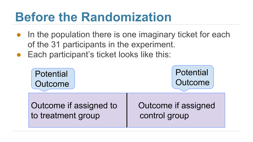
After the randomization, we get to see the right half of a randomly selected set of tickets, and the left half of the remaining group.

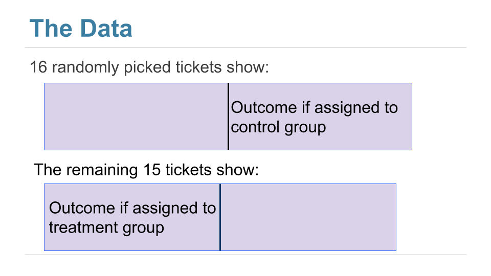
The table observed_outcomes collects the information about every patient’s potential outcomes, leaving the unobserved half of each “ticket” blank. (It’s just another way of thinking about the bta table, carrying the same information.)

Python

# Import dataset observed_outcomes.csv
observed_outcomes = pd.read_csv('https://github.com/ZacksAmber/Code/raw/master/Data%20Science/Data8/Data%20Sets/observed_outcomes.csv')
observed_outcomes

	Group	Outcome if assigned treatment	Outcome if assigned control
0	Control	Unknown	1
1	Control	Unknown	1
2	Control	Unknown	0
3	Control	Unknown	0
4	Control	Unknown	0
...	...	...	...
26	Treatment	0	Unknown
27	Treatment	0	Unknown
28	Treatment	0	Unknown
29	Treatment	0	Unknown
30	Treatment	0	Unknown

---

The Hypotheses

The question is whether the treatment does anything. In terms of the table observed_outcomes, the question is whether the distribution of the 31 “treatment” values in Column 1 (including the unknown ones) is different from the distribution of the 31 “control” values in Column 2 (again including the unknown ones).

Null Hypothesis: The distribution of all 31 potential “treatment” outcomes is the same as that of all 31 potential “control” outcomes. Botulinum toxin A does nothing different from saline; the difference in the two samples is just due to chance.

Alternative Hypothesis: The distribution of 31 potential “treatment” outcomes is different from that of the 31 control outcomes. The treatment does something different from the control.

There are 31 observed outcomes jointly in the two groups. If the null hypothesis were true, it wouldn’t matter which of those 31 outcomes were labeled “treatment” and which “control.” Any random subset of 16 out of the 31 values could be called “control” and the remaining 15 “treatment”.

We can simulate this. We can randomly permute the 31 values, split them into two groups of 16 and 15, and see how different the distributions in the two groups are. Since the data are zeros and ones, we can just see how different the two proportions are.

That’s exactly what we did for A/B testing in the previous section. Sample A is now the control group and Sample B the treatment group. We will carry out the test below showing the details of all the steps. You should confirm that they are the same as the steps carried out for A/B testing.

---

The Test Statistic

If the two group proportions are very different from each other, we will lean towards the alternative hypothesis that the two underlying distributions are different. So our test statistic will be the distance between the two group proportions, that is, the absolute value of the difference between them.

Large values of the test statistic will favor the alternative hypothesis over the null.

Since the two group proportions were 0.6 and 0.125, the observed value of the test statistic is $∣0.6−0.125∣=0.475$.

Python

# SELECT Group, AVG(Result) AS 'Result average' FROM bta GROUP BY Group;
bta.groupby('Group')['Result'].mean().reset_index(name='Result average')

	Group	Result average
0	Control	0.125
1	Treatment	0.600

Python

# Define observed distance
observed_proportions = bta.groupby('Group')['Result'].mean().reset_index(name='Result average').iloc[:, 1]
observed_distance = abs(observed_proportions[0] - observed_proportions[1])
observed_distance
# 0.475

As we have done before, we will define a function that takes the following arguments:

• the name of the table of data
• the column label of the numerical variable
• the column label of the group labels

and returns the absolute difference between the two group proportions.

Python

# Define function distance that returns the absolute difference between the two group proportions
def distance(table, label, group_label):
    proportions = table.groupby(group_label)[label].mean().reset_index(name='Result average').iloc[:, 1]
    return abs(proportions[0] - proportions[1])

Python

# Test function distance
distance(bta, 'Result', 'Group')
# 0.475

---

Predicting the Statistic Under the Null Hypothesis

We can simulate results under the null hypothesis, to see how our test statistic should come out if the null hypothesis is true.

---

Generating One Value of the Statistic

The simulation follows exactly the same process we used in the previous section. We start by randomly permuting the all group labels and then attaching the shuffled labels to the 0/1 results.

Python

# Shuffle the column 'Group'
shuffled_labels = bta['Group'].sample(n=len(bta), replace=False, random_state=2021).reset_index(drop=True)

Python

# One value
# Make new DataFrame bta_with_shuffled_labels from bta and add shuffled_labels to it.
bta_with_shuffled_labels = bta.copy()
bta_with_shuffled_labels['Shuffled Lable'] = shuffled_labels
bta_with_shuffled_labels

	Group	Result	Shuffled Lable
0	Control	1.0	Treatment
1	Control	1.0	Treatment
2	Control	0.0	Control
3	Control	0.0	Control
4	Control	0.0	Control
...	...	...	...
26	Treatment	0.0	Control
27	Treatment	0.0	Control
28	Treatment	0.0	Treatment
29	Treatment	0.0	Treatment
30	Treatment	0.0	Treatment

We can now find the distance between the two proportions after the group labels have been shuffled.

Python

# Test function distance
distance(bta_with_shuffled_labels, 'Result', 'Group')
# 0.475

Python

# Test function distance
distance(bta_with_shuffled_labels, 'Result', 'Shuffled Lable')
# 0.08750000000000002

---

Permutation Test

If we shuffled the labels again, how different would the new distance be? To answer this, we will define a function that simulates one simulated value of the distance under the hypothesis of random draws from the same underlying distribution. And then we will collect 20,000 such simulated values in an array.

You can see that we are doing exactly what we did in our previous examples of the permutation test.

Python

# Define function one_simulated_distance that generates one value
def one_simulated_distance(table, label, group_label):
    shuffled_labels = table[group_label].sample(n=len(table), replace=False).reset_index(drop=True)
    shuffled_table = table.copy()
    shuffled_table['Shuffled Label'] = shuffled_labels
    return distance(shuffled_table, label, 'Shuffled Label') 

Python

# Simulation: Permutation Test
distances = np.array([])

repetitions = 20000
for i in np.arange(repetitions):
    new_distance = one_simulated_distance(bta, 'Result', 'Group')
    distances = np.append(distances, new_distance)

distances = pd.DataFrame({'Distance': distances})
distances

	Distance
0	0.216667
1	0.087500
2	0.170833
3	0.170833
4	0.041667
...	...
19995	0.345833
19996	0.041667
19997	0.345833
19998	0.041667
19999	0.041667

---

Conclusion of the Test

The DataFrame distances contains 20,000 values of our test statistic simulated under the null hypothesis.

To find the P-value of the test, remember that large values of the test statistic favor the alternative hypothesis. So the empirical P-value is the proportion of simulated statistics that were equal to or larger than the observed statistic.

Python

# Empirical P-value
empirical_P = np.count_nonzero(distances >= observed_distance) / repetitions
empirical_P
# 0.0095

This is a small P-value. The observed statistic, shown as the red dot below, is in the tail of the empirical histogram of the test statistic generated under the null hypothesis.

The result is statistically significant. The test favors the alternative hypothesis over the null. The evidence supports the hypothesis that the treatment is doing something.

Python

# Histogram
fig = px.histogram(distances, 
                   histnorm='percent', 
                   x='Distance', 
                   color_discrete_sequence=['rgb(71, 92, 118)'], 
                   opacity=0.9)
# Set bins
fig.update_traces(xbins=dict(start=0, end=0.6, size=0.1))
# Set layout
fig.update_layout(yaxis_title='Percent', 
                  title='Prediction Under the Null Hypothesis')
# Add observed age difference
fig.add_trace(
    go.Scatter(
        mode='markers',
        x=[observed_distance],
        y=[0],
        marker=dict(
            color='red',
            size=8,
        ),
        showlegend=False,
    )
)
# Add annotation to observed distance
fig.add_annotation(x=observed_distance, # arrows' head
                   y=1, # arrows' head
                   ax=observed_distance, # arrows' tail
                   ay=15, # arrows' tail
                   xref='x',
                   yref='y',
                   axref='x',
                   ayref='y',
                   arrowhead=2, # arrow head's type
                   arrowsize=2, 
                   text='Observed Distance: '+str(observed_distance), # if you want only the arrow, text=''
                   showarrow=True)
# Add annotation to Empirical P-value
fig.add_annotation(x=observed_distance, # arrows' head
                   y=50, # arrows' head
                   xref='x',
                   yref='y',
                   text='Empirical P-value: '+str(empirical_P),
                   showarrow=False)

fig.show()
# fig.write_image('fig.svg')
# ![](https://raw.githubusercontent.com/ZacksAmber/PicGo/master/img/20210409172430.svg)

The study reports a P-value of 0.009, or 0.9%, which is not far from our empirical value.

---

Causality

Because the trials were randomized, the test is evidence that the treatment causes the difference. The random assignment of patients to the two groups ensures that there is no confounding variable that could affect the conclusion of causality.

If the treatment had not been randomly assigned, our test would still point toward an association between the treatment and back pain outcomes among our 31 patients. But beware: without randomization, this association would not imply that the treatment caused a change in back pain outcomes. For example, if the patients themselves had chosen whether to administer the treatment, perhaps the patients experiencing more pain would be more likely to choose the treatment and more likely to experience some reduction in pain even without medication. Pre-existing pain would then be a confounding factor in the analysis.

---

A Meta-Analysis

While the RCT does provide evidence that the botulinum toxin A treatment helped patients, a study of 31 patients isn’t enough to establish the effectiveness of a medical treatment. This is not just because of the small sample size. Our results in this section are valid for the 31 patients in the study, but we are really interested in the population of all possible patients. If the 31 patients were a random sample from that larger population, our confidence interval would be valid for that population. But they were not a random sample.

In 2011, a group of researchers performed a meta-analysis of the studies on the treatment. That is, they identified all the available studies of such treatments for low-back pain and summarized the collated results.

There were several studies but not many could be included in a scientifically sound manner: “We excluded evidence from nineteen studies due to non-randomisation, incomplete or unpublished data.” Only three randomized controlled trials remained, one of which is the one we have studied in this section. The meta-analysis gave it the highest assessment among all the studies (LBP stands for low-back pain): “We identified three studies that investigated the merits of BoNT for LBP, but only one had a low risk of bias and evaluated patients with non-specific LBP (N = 31).”

Putting it all together, the meta-analysis concluded, “There is low quality evidence that BoNT injections improved pain, function, or both better than saline injections and very low quality evidence that they were better than acupuncture or steroid injections. … Further research is very likely to have an important impact on the estimate of effect and our confidence in it. Future trials should standardize patient populations, treatment protocols and comparison groups, enlist more participants and include long-term outcomes, cost-benefit analysis and clinical relevance of findings.”

It takes a lot of careful work to establish that a medical treatment has a beneficial effect. Knowing how to analyze randomized controlled trials is a crucial part of this work. Now that you know how to do that, you are well positioned to help medical and other professions establish cause-and-effect relations.

---

Estimation

Estimation
Program: Data8-13.ipynb

In the previous chapter we began to develop ways of inferential thinking. In particular, we learned how to use data to decide between two hypotheses about the world. But often we just want to know how big something is.

For example, in an earlier chapter we investigated how many warplanes the enemy might have. In an election year, we might want to know what percent of voters favor a particular candidate. To assess the current economy, we might be interested in the median annual income of households in the United States.

In this chapter, we will develop a way to estimate an unknown parameter. Remember that a parameter is a numerical value associated with a population.

To figure out the value of a parameter, we need data. If we have the relevant data for the entire population, we can simply calculate the parameter.

But if the population is very large – for example, if it consists of all the households in the United States – then it might be too expensive and time-consuming to gather data from the entire population. In such situations, data scientists rely on sampling at random from the population.

This leads to a question of inference: How to make justifiable conclusions about the unknown parameter, based on the data in the random sample? We will answer this question by using inferential thinking.

A statistic based on a random sample can be a reasonable estimate of an unknown parameter in the population. For example, you might want to use the median annual income of sampled households as an estimate of the median annual income of all households in the U.S.

But the value of any statistic depends on the sample, and the sample is based on random draws. So every time data scientists come up with an estimate based on a random sample, they are faced with a question:

“How different could this estimate have been, if the sample had come out differently?”

In this chapter you will learn one way of answering this question. The answer will give you the tools to estimate a numerical parameter and quantify the amount of error in your estimate.

We will start with a preliminary about percentiles. The most famous percentile is the median, often used in summaries of income data. Other percentiles will be important in the method of estimation that we are about to develop. So we will start by defining percentiles carefully.

---

13.1. Percentiles

Numerical data can be sorted in increasing or decreasing order. Thus the values of a numerical data set have a rank order. A percentile is the value at a particular rank.

For example, if your score on a test is on the 95th percentile, a common interpretation is that only 5% of the scores were higher than yours. The median is the 50th percentile; it is commonly assumed that 50% the values in a data set are above the median.

But some care is required in giving percentiles a precise definition that works for all ranks and all lists. To see why, consider an extreme example where all the students in a class score 75 on a test. Then 75 is a natural candidate for the median, but it’s not true that 50% of the scores are above 75. Also, 75 is an equally natural candidate for the 95th percentile or the 25th or any other percentile. Ties – that is, equal data values – have to be taken into account when defining percentiles.

You also have to be careful about exactly how far up the list to go when the relevant index isn’t clear. For example, what should be the 87th percentile of a collection of 10 values? The 8th value of the sorted collection, or the 9th, or somewhere in between?

In this section, we will give a definition that works consistently for all ranks and all lists.

---

A Numerical Example

Before giving a general definition of all percentiles, we will define the 80th percentile of a collection of values to be the smallest value in the collection that is at least as large as 80% of all of the values.

For example, let’s consider the sizes of the five largest continents – Africa, Antarctica, Asia, North America, and South America – rounded to the nearest million square miles.

Python

# Continents size
sizes = np.array([12, 17, 6, 9, 7])

The 80th percentile is the smallest value that is at least as large as 80% of the elements of sizes, that is, four-fifths of the five elements. That’s 12:

Python

np.sort(sizes)
# array([ 6,  7,  9, 12, 17])

The 80th percentile is a value on the list, namely 12. You can see that 80% of the values are less than or equal to it, and that it is the smallest value on the list for which this is true.

Analogously, the 70th percentile is the smallest value in the collection that is at least as large as 70% of the elements of sizes. Now 70% of 5 elements is “3.5 elements”, so the 70th percentile is the 4th element on the list. That’s 12, the same as the 80th percentile for these data.

---

The percentile function

The np.percentile function takes three arguments: a array, a rank between 0 and 100, and interpolation. It returns the corresponding percentile of the array.

• interpolation: {‘linear’, ‘lower’, ‘higher’, ‘midpoint’, ‘nearest’}
• This optional parameter specifies the interpolation method to use when the desired percentile lies between two data points i < j:
• ‘linear’: i + (j - i) * fraction, where fraction is the fractional part of the index surrounded by i and j.
• ‘lower’: i.
• ‘higher’: j.
• ‘nearest’: i or j, whichever is nearest.
• ‘midpoint’: (i + j) / 2.

numpy.percentile
numpy.percentile() in python

Python

np.percentile(sizes, 70, interpolation='higher')
# 12

In this example, the 9 is 60th percentile and 12 is 80th percentile.

---

The General Definition

Let $p$ be a number between 0 and 100. The $p$th percentile of a collection is the smallest value in the collection that is at least as large as $p$% of all the values.

By this definition, any percentile between 0 and 100 can be computed for any collection of values, and it is always an element of the collection.

In practical terms, suppose there are $n$ elements in the collection. To find the $p$th percentile:

• Sort the collection in increasing order.
• Find $p$% of $n$: $(p/100)\times n$. Call that $k$.
• If $k$ is an integer, take the $k$th element of the sorted collection.
• If $k$ is not an integer, round it up to the next integer, and take that element of the sorted collection.

---

Example

The table scores_and_section contains one row for each student in a class of 359 students. The columns are the student’s discussion section and midterm score.

Python

# Import dataset scores_by_section.csv
scores_by_sections = pd.read_csv('https://github.com/ZacksAmber/Code/raw/master/Data%20Science/Data8/Data%20Sets/scores_by_section.csv')
scores_by_sections

	Section	Midterm
0	1	22
1	2	12
2	2	23
3	2	14
4	1	20
...	...	...
354	5	24
355	2	16
356	2	17
357	12	16
358	10	14

Python

# Histogram
fig = px.histogram(scores_by_sections, 
                   histnorm='percent', 
                   x='Midterm', 
                   color_discrete_sequence=['rgb(71, 92, 118)'], 
                   opacity=0.9)
# Set bins
fig.update_traces(xbins=dict(start=0, end=25, size=1))
# Set layout
fig.update_layout(yaxis_title='Percent')
fig.show()
# fig.write_image('fig.svg')
# ![](https://raw.githubusercontent.com/ZacksAmber/PicGo/master/img/20210409233630.svg)

What was the 85th percentile of the scores? To use the percentile function, create an array scores containing the midterm scores, and find the 85th percentile:

Python

# Create array scores
scores = scores_by_sections.Midterm
# Get the 85th percentile of the scores
np.percentile(scores, 85, interpolation='higher')
# 22

According to the percentile function, the 85th percentile was 22. To check that this is consistent with our new definition, let’s apply the definition directly.

First, put the scores in increasing order:

Python

# Sort Midterm
sorted_scores = np.sort(scores_by_sections.Midterm)
len(sorted_scores)
# 359

There are 359 scores in the array. So next, find 85% of 359, which is 305.15.

Python

0.85 * 359
# 305.15

That’s not an integer. By our definition, the 85th percentile is the 306th element of sorted_scores, which, by Python’s indexing convention, is item 305 of the array.

Python

# Get the 85% of sorted_scores.
# Don't forget the 1st item in Python list is index 0.
sorted_scores[int(0.85*359)]
# 22

That’s the same as the answer we got by using percentile. In future, we will just use np.percentile.

---

Quartiles

The first quartile of a numercial collection is the 25th percentile. The terminology arises from the first quarter. The second quartile is the median, and the third quartile is the 75th percentile.

For our scores data, those values are:

Python

# 1st quartiles
np.percentile(scores, 25, interpolation='higher')
# 11

Python

# 2nd quartiles
np.percentile(scores, 50, interpolation='higher')
# 16

Python

# 3rd quartiles
np.percentile(scores, 75, interpolation='higher')
# 20

Tips:

• 0 quartile = 0 quantile = 0 percentile
• 1 quartile = 0.25 quantile = 25 percentile
• 2 quartile = .5 quantile = 50 percentile (median)
• 3 quartile = .75 quantile = 75 percentile
• 4 quartile = 1 quantile = 100 percentile

---

13.2. The Bootstrap

A data scientist is using the data in a random sample to estimate an unknown parameter. She uses the sample to calculate the value of a statistic that she will use as her estimate.

Once she has calculated the observed value of her statistic, she could just present it as her estimate and go on her merry way. But she’s a data scientist. She knows that her random sample is just one of numerous possible random samples, and thus her estimate is just one of numerous plausible estimates.

By how much could those estimates vary? To answer this, it appears as though she needs to draw another sample from the population, and compute a new estimate based on the new sample. But she doesn’t have the resources to go back to the population and draw another sample.

It looks as though the data scientist is stuck.

Fortunately, a brilliant idea called the bootstrap can help her out. Since it is not feasible to generate new samples from the population, the bootstrap generates new random samples by a method called resampling: the new samples are drawn at random from the original sample.

In this section, we will see how and why the bootstrap works. In the rest of the chapter, we will use the bootstrap for inference.

---

Employee Compensation in the City of San Francisco

SF OpenData is a website where the City and County of San Francisco make some of their data publicly available. One of the data sets contains compensation data for employees of the City. These include medical professionals at City-run hospitals, police officers, fire fighters, transportation workers, elected officials, and all other employees of the City.

Compensation data for the calendar year 2015 are in the table sf2015.

Python

# Import dataset san_francisco_2015.csv
sf2015 = pd.read_csv('https://raw.githubusercontent.com/ZacksAmber/Code/master/Data%20Science/Data8/Data%20Sets/san_francisco_2015.csv')
sf2015

	Year Type	Year	Organization Group Code	Organization Group	Department Code	Department	Union Code	Union	Job Family Code	Job Family	...	Employee Identifier	Salaries	Overtime	Other Salaries	Total Salary	Retirement	Health/Dental	Other Benefits	Total Benefits	Total Compensation
0	Calendar	2015	2	Public Works, Transportation & Commerce	WTR	PUC Water Department	21.0	Prof & Tech Engineers - Miscellaneous, Local 21	2400	Lab, Pharmacy & Med Techs	...	21538	82146.04	0.00	0.00	82146.04	16942.21	12340.88	6337.73	35620.82	117766.86
1	Calendar	2015	2	Public Works, Transportation & Commerce	DPW	General Services Agency - Public Works	12.0	Carpet, Linoleum and Soft Tile Workers, Local 12	7300	Journeyman Trade	...	5459	32165.75	973.19	848.96	33987.90	0.00	4587.51	2634.42	7221.93	41209.83
2	Calendar	2015	4	Community Health	DPH	Public Health	790.0	SEIU - Miscellaneous, Local 1021	1600	Payroll, Billing & Accounting	...	41541	71311.00	5757.98	0.00	77068.98	14697.59	12424.50	6370.06	33492.15	110561.13
3	Calendar	2015	4	Community Health	DPH	Public Health	351.0	Municipal Executive Association - Miscellaneous	0900	Management	...	26718	28430.25	0.00	763.07	29193.32	0.00	4223.14	5208.51	9431.65	38624.97
4	Calendar	2015	2	Public Works, Transportation & Commerce	MTA	Municipal Transportation Agency	790.0	SEIU - Miscellaneous, Local 1021	8200	Protection & Apprehension	...	45810	7948.75	0.00	0.00	7948.75	0.00	2873.17	616.24	3489.41	11438.16
...	...	...	...	...	...	...	...	...	...	...	...	...	...	...	...	...	...	...	...	...	...
42984	Calendar	2015	2	Public Works, Transportation & Commerce	MTA	Municipal Transportation Agency	200.0	Transportation Workers, Local 200	9100	Street Transit	...	13250	80691.52	11865.91	3290.29	95847.72	16909.07	12244.02	7788.00	36941.09	132788.81
42985	Calendar	2015	4	Community Health	DPH	Public Health	791.0	SEIU - Staff and Per Diem Nurses, Local 1021	2300	Nursing	...	14845	7559.66	0.00	0.00	7559.66	153.74	0.00	2132.23	2285.97	9845.63
42986	Calendar	2015	1	Public Protection	POL	Police	911.0	Police Officers' Association	Q000	Police Services	...	40128	48843.58	2965.85	3316.21	55125.64	11047.55	6212.24	910.16	18169.95	73295.59
42987	Calendar	2015	6	General Administration & Finance	ADM	General Services Agency - City Admin	39.0	Stationary Engineers, Local 39	7300	Journeyman Trade	...	48315	16319.20	0.00	0.00	16319.20	0.00	2389.32	1264.85	3654.17	19973.37
42988	Calendar	2015	6	General Administration & Finance	ADM	General Services Agency - City Admin	856.0	Teamsters - Miscellaneous, Local 856	3300	Park & Zoo	...	17657	34267.20	344.85	1256.89	35868.94	8643.54	8458.22	2842.20	19943.96	55812.90

There is one row for each of 42,989 employees. There are numerous columns containing information about City departmental affiliation and details of the different parts of the employee’s compensation package. Here is the row correspoding to the late Edward Lee, the Mayor at that time.

Python

# SELECT * FROM sf2015 WHERE Job = 'Mayor';
sf2015[sf2015.Job == 'Mayor']

	Year Type	Year	Organization Group Code	Organization Group	Department Code	Department	Union Code	Union	Job Family Code	Job Family	...	Employee Identifier	Salaries	Overtime	Other Salaries	Total Salary	Retirement	Health/Dental	Other Benefits	Total Benefits	Total Compensation
3335	Calendar	2015	6	General Administration & Finance	MYR	Mayor	556.0	Elected Officials	1100	Administrative & Mgmt (Unrep)	...	22433	288963.55	0.0	0.0	288963.55	58117.03	12424.5	20292.95	90834.48	379798.03

We are going to study the final column, Total Compensation. That’s the employee’s salary plus the City’s contribution towards his/her retirement and benefit plans.

Financial packages in a calendar year can sometimes be hard to understand as they depend on the date of hire, whether the employee is changing jobs within the City, and so on. For example, the lowest values in the Total Compensation column look a little strange.

Python

# SELECT * FROM sf2015 ORDER BY 'Total Compensation' ASC;
sf2015.sort_values('Total Compensation')

	Year Type	Year	Organization Group Code	Organization Group	Department Code	Department	Union Code	Union	Job Family Code	Job Family	...	Employee Identifier	Salaries	Overtime	Other Salaries	Total Salary	Retirement	Health/Dental	Other Benefits	Total Benefits	Total Compensation
27308	Calendar	2015	1	Public Protection	FIR	Fire Department	798.0	Firefighters - Miscellaneous, Local 798	H000	Fire Services	...	43833	0.00	0.00	0.00	0.00	0.00	0.00	-423.76	-423.76	-423.76
15746	Calendar	2015	4	Community Health	DPH	Public Health	790.0	SEIU - Miscellaneous, Local 1021	9900	Public Service Aide	...	27871	-292.40	0.00	0.00	-292.40	0.00	-95.58	-22.63	-118.21	-410.61
24576	Calendar	2015	1	Public Protection	JUV	Juvenile Probation	790.0	SEIU - Miscellaneous, Local 1021	8300	Correction & Detention	...	10517	0.00	0.00	0.00	0.00	0.00	0.00	-159.12	-159.12	-159.12
42982	Calendar	2015	6	General Administration & Finance	CPC	City Planning	21.0	Prof & Tech Engineers - Miscellaneous, Local 21	1000	Information Systems	...	18961	0.00	0.00	0.00	0.00	0.00	0.00	-26.53	-26.53	-26.53
23310	Calendar	2015	6	General Administration & Finance	CPC	City Planning	21.0	Prof & Tech Engineers - Miscellaneous, Local 21	5200	Professional Engineering	...	19387	0.00	0.00	0.00	0.00	0.00	0.00	-9.51	-9.51	-9.51
...	...	...	...	...	...	...	...	...	...	...	...	...	...	...	...	...	...	...	...	...	...
5171	Calendar	2015	4	Community Health	DPH	Public Health	351.0	Municipal Executive Association - Miscellaneous	0900	Management	...	1523	256098.01	0.00	82292.31	338390.32	51977.53	11468.77	20963.32	84409.62	422799.94
17805	Calendar	2015	2	Public Works, Transportation & Commerce	AIR	Airport Commission	351.0	Municipal Executive Association - Miscellaneous	0900	Management	...	17356	326764.01	0.00	0.00	326764.01	65806.33	12424.50	21691.23	99922.06	426686.07
499	Calendar	2015	6	General Administration & Finance	ADM	General Services Agency - City Admin	164.0	Physicians and Dentists - Miscellaneous	2500	Med Therapy & Auxiliary	...	13746	279311.03	9046.92	56742.56	345100.51	56211.61	12424.50	13482.66	82118.77	427219.28
13194	Calendar	2015	6	General Administration & Finance	ADM	General Services Agency - City Admin	164.0	Physicians and Dentists - Miscellaneous	2500	Med Therapy & Auxiliary	...	1016	279311.10	3829.36	114433.58	397574.04	56211.64	12424.50	14299.10	82935.24	480509.28
19177	Calendar	2015	6	General Administration & Finance	RET	Retirement System	351.0	Municipal Executive Association - Miscellaneous	1100	Administrative & Mgmt (Unrep)	...	46881	507831.60	0.00	0.00	507831.60	105052.98	12424.50	23566.16	141043.64	648875.24

For clarity of comparison, we will focus our attention on those who had at least the equivalent of a half-time job for the whole year. At a minimum wage of about 10 dollars per hour, and 20 hours per week for 52 weeks, that’s a salary of about 10,000 dollars.

Python

# SELECT * FROM sf2015 WHERE Salaries > 10000;
sf2015 = sf2015[sf2015.Salaries > 10000]
sf2015

Python

len(sf2015)
# 36569

---

Population and Parameter

Let this table of just over 36,500 rows be our population. Here is a histogram of the total compensations.

Python

# Histogram
fig = px.histogram(sf2015, 
                   histnorm='percent', 
                   x='Total Compensation', 
                   color_discrete_sequence=['rgb(71, 92, 118)'], 
                   opacity=0.9)
# Set bins
fig.update_traces(xbins=dict(start=0, end=700000, size=25000))
# Set layout
fig.update_layout(yaxis_title='Percent', 
                  title='Population')
fig.show()
# fig.write_image('fig.svg')
# ![](https://raw.githubusercontent.com/ZacksAmber/PicGo/master/img/20210410155921.svg)

While most of the values are below USD 300k, a few are quite a bit higher. For example, the total compensation of the Chief Investment Officer was almost USD 650k. That is why the horizontal axis stretches to USD 700k.

Python

# Filter the highest two 'Total Compensation'
sf2015.sort_values('Total Compensation', ascending=False).iloc[:2, :]

	Year Type	Year	Organization Group Code	Organization Group	Department Code	Department	Union Code	Union	Job Family Code	Job Family	...	Employee Identifier	Salaries	Overtime	Other Salaries	Total Salary	Retirement	Health/Dental	Other Benefits	Total Benefits	Total Compensation
19177	Calendar	2015	6	General Administration & Finance	RET	Retirement System	351.0	Municipal Executive Association - Miscellaneous	1100	Administrative & Mgmt (Unrep)	...	46881	507831.6	0.00	0.00	507831.60	105052.98	12424.5	23566.16	141043.64	648875.24
13194	Calendar	2015	6	General Administration & Finance	ADM	General Services Agency - City Admin	164.0	Physicians and Dentists - Miscellaneous	2500	Med Therapy & Auxiliary	...	1016	279311.1	3829.36	114433.58	397574.04	56211.64	12424.5	14299.10	82935.24	480509.28

Now let the parameter be the median of the total compensations.

Since we have the luxury of having all of the data from the population, we can simply calculate the parameter:

Python

# Calculate the median 'Total Compensation' of sf2015
pop_median = np.percentile(sf2015['Total Compensation'], q=50, interpolation='higher')
pop_median
# 110305.79

The median total compensation of all employees was just over USD 110,300.

From a practical perspective, there is no reason for us to draw a sample to estimate this parameter since we simply know its value. But in this section we are going to pretend we don’t know the value, and see how well we can estimate it based on a random sample.

In later sections, we will come down to earth and work in situations where the parameter is unknown. For now, we are all-knowing.

---

A Random Sample and an Estimate

Let us draw a sample of 500 employees at random without replacement, and let the median total compensation of the sampled employees serve as our estimate of the parameter.

Python

# Randomly select 500 samples from population sf2015
our_sample = sf2015.sample(n=500, replace=False, random_state=2021).reset_index(drop=True)
our_sample

	Year Type	Year	Organization Group Code	Organization Group	Department Code	Department	Union Code	Union	Job Family Code	Job Family	...	Employee Identifier	Salaries	Overtime	Other Salaries	Total Salary	Retirement	Health/Dental	Other Benefits	Total Benefits	Total Compensation
0	Calendar	2015	2	Public Works, Transportation & Commerce	PRT	Port	351.0	Municipal Executive Association - Miscellaneous	0900	Management	...	10539	158707.06	0.00	0.00	158707.06	31940.40	12424.50	17692.59	62057.49	220764.55
1	Calendar	2015	2	Public Works, Transportation & Commerce	DBI	Department of Building Inspection	790.0	SEIU - Miscellaneous, Local 1021	1400	Clerical, Secretarial & Steno	...	20480	21006.10	0.00	0.00	21006.10	5419.57	5256.52	1701.15	12377.24	33383.34
2	Calendar	2015	2	Public Works, Transportation & Commerce	MTA	Municipal Transportation Agency	253.0	Transport Workers - Transit Operators, Local 2...	9100	Street Transit	...	39145	66609.43	4528.33	5221.11	76358.87	19694.69	13128.88	5699.13	38522.70	114881.57
3	Calendar	2015	2	Public Works, Transportation & Commerce	DBI	Department of Building Inspection	38.0	Plumbers and Pipefitters, Local 38	6200	Public Safety Inspection	...	2641	137101.06	0.00	7508.05	144609.11	29090.04	12424.50	10117.32	51631.86	196240.97
4	Calendar	2015	1	Public Protection	DAT	District Attorney	311.0	Municipal Attorneys' Association	8100	Legal & Court	...	50797	112563.61	0.00	1500.00	114063.61	22831.29	11884.39	8579.31	43294.99	157358.60
...	...	...	...	...	...	...	...	...	...	...	...	...	...	...	...	...	...	...	...	...	...
495	Calendar	2015	1	Public Protection	FIR	Fire Department	799.0	Firefighters - Chiefs/Fire Boat Workers, Local...	H000	Fire Services	...	31171	180314.38	97782.52	27305.16	305402.06	40610.70	15196.12	4627.67	60434.49	365836.55
496	Calendar	2015	2	Public Works, Transportation & Commerce	WTR	PUC Water Department	3.0	Operating Engineers - Miscellaneous, Local 3	7300	Journeyman Trade	...	27186	91368.68	0.00	0.00	91368.68	18790.78	12026.16	7339.97	38156.91	129525.59
497	Calendar	2015	5	Culture & Recreation	AAM	Asian Art Museum	790.0	SEIU - Miscellaneous, Local 1021	8200	Protection & Apprehension	...	37275	11967.79	0.00	0.00	11967.79	0.00	2859.73	927.81	3787.54	15755.33
498	Calendar	2015	4	Community Health	DPH	Public Health	791.0	SEIU - Staff and Per Diem Nurses, Local 1021	2300	Nursing	...	45546	20160.61	0.00	833.74	20994.35	0.00	1574.50	1626.94	3201.44	24195.79
499	Calendar	2015	1	Public Protection	FIR	Fire Department	798.0	Firefighters - Miscellaneous, Local 798	H000	Fire Services	...	49093	112108.33	3449.17	18686.95	134244.45	24764.36	15044.40	2240.67	42049.43	176293.88

Python

# Histogram
fig = px.histogram(our_sample, 
                   histnorm='percent', 
                   x='Total Compensation', 
                   range_x=[0, 700000], # Forcibly set x domain from 0 to 700k
                   color_discrete_sequence=['rgb(71, 92, 118)'], 
                   opacity=0.9)
# Set bins
fig.update_traces(xbins=dict(start=0, end=700000, size=25000))
# Set layout
fig.update_layout(yaxis_title='Percent', 
                  title='Sample Size = 500')
fig.show()
# fig.write_image('fig.svg')
# ![](https://raw.githubusercontent.com/ZacksAmber/PicGo/master/img/20210410161008.svg)

Python

# Calculate the median 'Total Compensation' of our_sample
est_median = np.percentile(our_sample['Total Compensation'], q=50, interpolation='higher')
est_median
# 112176.02

The sample size is large. By the law of averages, the distribution of the sample resembles that of the population, and consequently the sample median is not very far from the population median (though of course it is not exactly the same).

So now we have one estimate of the parameter. But had the sample come out differently, the estimate would have had a different value. We would like to be able to quantify the amount by which the estimate could vary across samples. That measure of variability will help us measure how accurately we can estimate the parameter.

To see how different the estimate would be if the sample had come out differently, we could just draw another sample from the population, but that would be cheating. We are trying to mimic real life, in which we won’t have all the population data at hand.

Somehow, we have to get another random sample without sampling from the population.

---

The Bootstrap: Resampling from the Sample

What we do have is a large random sample from the population. As we know, a large random sample is likely to resemble the population from which it is drawn. This observation allows data scientists to lift themselves up by their own bootstraps: the sampling procedure can be replicated by sampling from the sample.

Here are the steps of the bootstrap method for generating another random sample that resembles the population:

• Treat the original sample as if it were the population.
• Draw from the sample, at random with replacement, the same number of times as the original sample size.

It is important to resample the same number of times as the original sample size. The reason is that the variability of an estimate depends on the size of the sample. Since our original sample consisted of 500 employees, our sample median was based on 500 values. To see how different the sample could have been, we have to compare it to the median of other samples of size 500.

If we drew 500 times at random without replacement from our sample of size 500, we would just get the same sample back. By drawing with replacement, we create the possibility for the new samples to be different from the original, because some employees might be drawn more than once and others not at all.

Why is this a good idea? By the law of averages, the distribution of the original sample is likely to resemble the population, and the distributions of all the “resamples” are likely to resemble the original sample. So the distributions of all the resamples are likely to resemble the population as well.

---

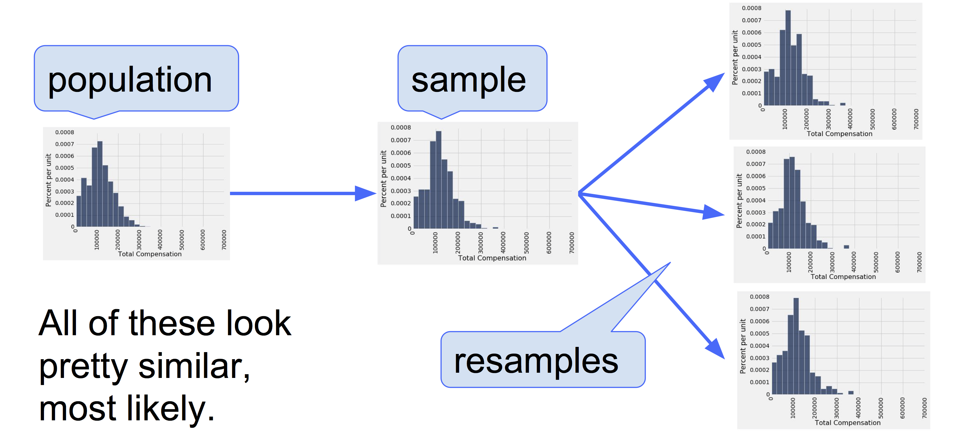
A Resampled Median

Recall that when the sample method is used with specifying a sample size. That’s perfect for the bootstrap! Here is one new sample drawn from the original sample, and the corresponding sample median.

Python

# Resamaple once
resample_1 = our_sample.sample(n=500, replace=True, random_state=2021).reset_index(drop=True)

Python

# Histogram
fig = px.histogram(resample_1, 
                   histnorm='percent', 
                   x='Total Compensation', 
                   range_x=[0, 700000], # Forcibly set x domain from 0 to 700k
                   color_discrete_sequence=['rgb(71, 92, 118)'], 
                   opacity=0.9)
# Set bins
fig.update_traces(xbins=dict(start=0, end=700000, size=25000))
# Set layout
fig.update_layout(yaxis_title='Percent', 
                  title='resample_1')
fig.show()
# fig.write_image('fig.svg')
# ![](https://raw.githubusercontent.com/ZacksAmber/PicGo/master/img/20210410162931.svg)

Python

# Calculate median 'Total Compensation' of resample_1
resampled_median_1 = np.percentile(resample_1['Total Compensation'], q=50, interpolation='higher')
resampled_median_1
# 111721.42

By resampling, we have another estimate of the population median. By resampling again and again, we will get many such estimates, and hence an empirical distribution of the estimates.

Python

# Resamaple again
resample_2 = our_sample.sample(n=500, replace=True, random_state=2022).reset_index(drop=True)
# Calculate median 'Total Compensation' of resample_2
resampled_median_2 = np.percentile(resample_2['Total Compensation'], q=50, interpolation='higher')
resampled_median_2
# 111700.15

---

Bootstrap Empirical Distribution of the Sample Median

Let us define a function bootstrap_median that takes our original sample, the label of the column containing the variable, and the number of bootstrap samples we want to take, and returns an array of the corresponding resampled medians.

Each time we resample and find the median, we replicate the bootstrap process. So the number of bootstrap samples will be called the number of replications.

Python

# Define function bootstrap_median return array of bootstrapped sample medians
def bootstrap_median(original_sample, label, replications):
    """Returns an array of bootstrapped sample medians:
    original_sample: table containing the original sample
    label: label of column containing the variable
    replications: number of bootstrap samples
    """
    just_one_column = original_sample[label] # our_sample['Total Compensation']
    sample_size = len(original_sample)
    medians = np.array([])
    for i in np.arange(replications):
        bootstrap_sample = just_one_column.sample(n=sample_size, replace=True).reset_index(drop=True)
        resampled_median = np.percentile(bootstrap_sample, q=50, interpolation='higher')
        medians = np.append(medians, resampled_median)
        
    return medians

We now replicate the bootstrap process 5,000 times. The array bstrap_medians contains the medians of all 5,000 bootstrap samples. Notice that the code takes longer to run than our previous code. It has a lot of resampling to do!

Python

# Resample 5,000 times
bstrap_medians = bootstrap_median(our_sample, 'Total Compensation', 5000)

# Convert bstrap_medians from array to DataFrame
bstrap_medians = pd.DataFrame({'Bootstrap Sample Median': bstrap_medians})

Here is the histogram of the 5000 medians. The red dot is the population parameter: it is the median of the entire population, which we happen to know but did not use in the bootstrap process.

Python

# Histogram
fig = px.histogram(bstrap_medians, 
                   histnorm='percent', 
                   x='Bootstrap Sample Median', 
                   color_discrete_sequence=['rgb(71, 92, 118)'], 
                   opacity=0.9)
# Set bins
fig.update_traces(xbins=dict(start=100000, end=130000, size=2500))
# Set layout
fig.update_layout(yaxis_title='Percent', 
                  title='Bootstrap Empirical Distribution of the Sample Median')
# Mark pop_median
fig.add_trace(
    go.Scatter(
        mode='markers',
        x=[pop_median],
        y=[0],
        marker=dict(
            color='red',
            size=8,
        ),
        showlegend=False,
    )
)
fig.show()
# fig.write_image('fig.svg')
# ![](https://raw.githubusercontent.com/ZacksAmber/PicGo/master/img/20210410165838.svg)

It is important to remember that the red dot is fixed: it is $110,305.79, the population median. The empirical histogram is the result of random draws, and will be situated randomly relative to the red dot.

Remember also that the point of all these computations is to estimate the population median, which is the red dot. Our estimates are all the randomly generated sampled medians whose histogram you see above. We want those estimates to contain the parameter – it they don’t, then they are off.

---

Do the Estimates Capture the Parameter?

How often does the empirical histogram of the resampled medians sit firmly over the red dot, and not just brush the dot with its tails? To answer this, we must define “sit firmly”. Let’s take that to mean “the middle 95% of the resampled medians contains the red dot”.

Here are the two ends of the “middle 95%” interval of resampled medians:

Python

# Define left
left = np.percentile(bstrap_medians, q=2.5, interpolation='higher')
left
# 106284.22

Python

# Define right
right = np.percentile(bstrap_medians, q=97.5, interpolation='higher')
right
# 116550.06

The population median of $110,305 is between these two numbers. The interval and the population median are shown on the histogram below.

Shapes in Python

Python

# Mark confidence interval 95%
fig.add_shape(type='line', x0=left, y0=0, x1=right, y1=0, line_color='gold')
fig.show()
# fig.write_image('fig.svg')
# ![](https://raw.githubusercontent.com/ZacksAmber/PicGo/master/img/20210410171009.svg)

The “middle 95%” interval of estimates captured the parameter in our example. But was that a fluke?

To see how frequently the interval contains the parameter, we have to run the entire process over and over again. Specifically, we will repeat the following process 100 times:

• Draw an original sample of size 500 from the population.
• Carry out 5,000 replications of the bootstrap process and generate the “middle 95%” interval of resampled medians.

We will end up with 100 intervals, and count how many of them contain the population median.

Spoiler alert: The statistical theory of the bootstrap says that the number should be around 95. It may be in the low 90s or high 90s, but not much farther off 95 than that.

Python

# THE BIG SIMULATION: This one takes several minutes.

# Generate 100 intervals, in the table intervals

left_ends = np.array([])
right_ends = np.array([])

total_comps = sf2015.loc[:, ['Total Compensation']]

for i in np.arange(100):
    first_sample = total_comps.sample(n=500, replace=False)
    medians = bootstrap_median(first_sample, 'Total Compensation', 5000)
    left_ends = np.append(left_ends, np.percentile(medians, q=2.5, interpolation='higher'))
    right_ends = np.append(right_ends, np.percentile(medians, q=97.5, interpolation='higher'))

intervals = pd.DataFrame(
    {'Left': left_ends,
    'Right': right_ends}
)    

The good intervals are those that contain the parameter we are trying to estimate. Typically the parameter is unknown, but in this section we happen to know what the parameter is.

Python

pop_median
# 110305.79

How many of the 100 intervals contain the population median? That’s the number of intervals where the left end is below the population median and the right end is above.

Python

intervals

	Left	Right
0	106676.06	119038.98
1	110398.67	122138.94
2	105493.67	114843.85
3	106895.71	118770.32
4	108364.09	121361.62
...	...	...
95	101720.31	113408.30
96	109813.47	121681.72
97	98853.33	114044.69
98	104235.05	114180.71
99	101052.62	113825.70

Python

# Count the qualified intervals
len(intervals[(intervals.Left < pop_median) & (intervals.Right > pop_median)])
# 96

It takes a few minutes to construct all the intervals, but try it again if you have the patience. Most likely, about 95 of the 100 intervals will be good ones: they will contain the parameter.

It’s hard to show you all the intervals on the horizontal axis as they have large overlaps – after all, they are all trying to estimate the same parameter. The graphic below shows each interval on the same axes by stacking them vertically. The vertical axis is simply the number of the replication from which the interval was generated.

The red line is where the parameter is. Good intervals cover the parameter; there are about 95 of these, typically.

If an interval doesn’t cover the parameter, it’s a dud. The duds are the ones where you can see “daylight” around the red line. There are very few of them – about 5, typically – but they do happen.

Any method based on sampling has the possibility of being off. The beauty of methods based on random sampling is that we can quantify how often they are likely to be off.

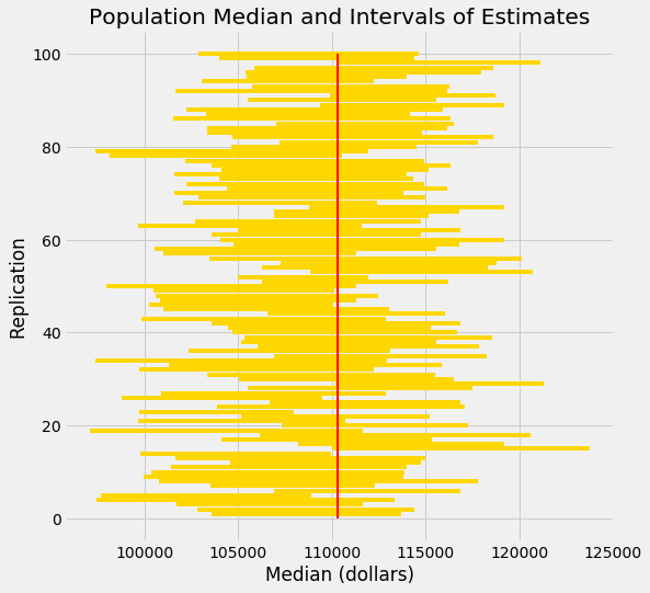
To summarize what the simulation shows, suppose you are estimating the population median by the following process:

• Draw a large random sample from the population.
• Bootstrap your random sample and get an estimate from the new random sample.
• Repeat the above step thousands of times, and get thousands of estimates.
• Pick off the “middle 95%” interval of all the estimates.

That gives you one interval of estimates. Now if you repeat the entire process 100 times, ending up with 100 intervals, then about 95 of those 100 intervals will contain the population parameter.

In other words, this process of estimation captures the parameter about 95% of the time.

You can replace 95% by a different value, as long as it’s not 100. Suppose you replace 95% by 80% and keep the sample size fixed at 500. Then your intervals of estimates will be shorter than those we simulated here, because the “middle 80%” is a smaller range than the “middle 95%”. Only about 80% of your intervals will contain the parameter.

---

13.3. Confidence Intervals

We have developed a method for estimating a parameter by using random sampling and the bootstrap. Our method produces an interval of estimates, to account for chance variability in the random sample. By providing an interval of estimates instead of just one estimate, we give ourselves some wiggle room.

In the previous example we saw that our process of estimation produced a good interval about 95% of the time, a “good” interval being one that contains the parameter. We say that we are 95% confident that the process results in a good interval. Our interval of estimates is called a 95% confidence interval for the parameter, and 95% is called the confidence level of the interval.

The situation in the previous example was a bit unusual. Because we happened to know the value of the parameter, we were able to check whether an interval was good or a dud, and this in turn helped us to see that our process of estimation captured the parameter about 95 out of every 100 times we used it.

But usually, data scientists don’t know the value of the parameter. That is the reason they want to estimate it in the first place. In such situations, they provide an interval of estimates for the unknown parameter by using methods like the one we have developed. Because of statistical theory and demonstrations like the one we have seen, data scientists can be confident that their process of generating the interval results in a good interval a known percent of the time.

---

Confidence Interval for a Population Median: Bootstrap Percentile Method

We will now use the bootstrap method to estimate an unknown population median. The data come from a sample of newborns in a large hospital system; we will treat it as if it were a simple random sample though the sampling was done in multiple stages. Stat Labs by Deborah Nolan and Terry Speed has details about a larger dataset from which this set is drawn.

The table baby contains the following variables for mother-baby pairs: the baby’s birth weight in ounces, the number of gestational days, the mother’s age in completed years, the mother’s height in inches, pregnancy weight in pounds, and whether or not the mother smoked during pregnancy.

Python

# Import dataset baby.csv
baby = pd.read_csv('https://github.com/ZacksAmber/Code/raw/master/Data%20Science/Data8/Data%20Sets/baby.csv')
baby

	Birth Weight	Gestational Days	Maternal Age	Maternal Height	Maternal Pregnancy Weight	Maternal Smoker
0	120	284	27	62	100	False
1	113	282	33	64	135	False
2	128	279	28	64	115	True
3	108	282	23	67	125	True
4	136	286	25	62	93	False
...	...	...	...	...	...	...
1169	113	275	27	60	100	False
1170	128	265	24	67	120	False
1171	130	291	30	65	150	True
1172	125	281	21	65	110	False
1173	117	297	38	65	129	False

Birth weight is an important factor in the health of a newborn infant – smaller babies tend to need more medical care in their first days than larger newborns. It is therefore helpful to have an estimate of birth weight before the baby is born. One way to do this is to examine the relationship between birth weight and the number of gestational days.

A simple measure of this relationship is the ratio of birth weight to the number of gestational days. The table ratios contains the first two columns of baby, as well as a column of the ratios. The first entry in that column was calculated as follows:

$$\frac{120\mbox{ ounces}}{284\mbox{ days}} \approx 0.4225 \mbox{ ounces per day}$$

Python

# Filter columns 'Birth Weight' and 'Gestational Days'
ratios = baby.loc[:, ['Birth Weight', 'Gestational Days']]
# Add column 'Ratio BW/GD'
ratios['Ratio BW/GD'] = ratios['Birth Weight']/ratios['Gestational Days']
ratios

	Birth Weight	Gestational Days	Ratio BW/GD
0	120	284	0.422535
1	113	282	0.400709
2	128	279	0.458781
3	108	282	0.382979
4	136	286	0.475524
...	...	...	...
1169	113	275	0.410909
1170	128	265	0.483019
1171	130	291	0.446735
1172	125	281	0.444840
1173	117	297	0.393939

Here is a histogram of the ratios.

Python

# Histogram
fig = px.histogram(ratios, 
                   histnorm='percent', 
                   x='Ratio BW/GD', 
                   color_discrete_sequence=['rgb(71, 92, 118)'], 
                   opacity=0.9)
# Set bins
fig.update_traces(xbins=dict(start=0, end=0.8, size=0.05))
# Set layout
fig.update_layout(yaxis_title='Percent')

fig.show()
# fig.write_image('fig.svg')
# ![](https://raw.githubusercontent.com/ZacksAmber/PicGo/master/img/20210415003714.svg)

At first glance the histogram looks quite symmetric, with the density at its maximum over the interval 4 ounces per day to 4.5 ounces per day. But a closer look reveals that some of the ratios were quite large by comparison. The maximum value of the ratios was just over 0.78 ounces per day, almost double the typical value.

Python

# Select the max 'Ratio BW/GD'
ratios.sort_values('Ratio BW/GD', ascending=False).iloc[[0], :]

	Birth Weight	Gestational Days	Ratio BW/GD
238	116	148	0.783784

The median gives a sense of the typical ratio because it is unaffected by the very large or very small ratios. The median ratio in the sample is about 0.429 ounces per day.

Python

# Select the median of 'Ratio BW/GD'
np.median(ratios['Ratio BW/GD'])
# 0.42907801418439717

But what was the median in the population? We don’t know, so we will estimate it.

Our method will be exactly the same as in the previous section. We will bootstrap the sample 5,000 times resulting in 5,000 estimates of the median. Our 95% confidence interval will be the “middle 95%” of all of our estimates.

Recall the function bootstrap_median defined in the previous section. We will call this function and construct a 95% confidence interval for the median ratio in the population. Remember that the table ratios contains the relevant data from our original sample.

Python

# Define function bootstrap_median return array of bootstrapped sample medians
def bootstrap_median(original_sample, label, replications):
    """Returns an array of bootstrapped sample medians:
    original_sample: table containing the original sample
    label: label of column containing the variable
    replications: number of bootstrap samples
    """
    just_one_column = original_sample[label]
    sample_size = len(original_sample)
    medians = np.array([])
    for i in np.arange(replications):
        bootstrap_sample = just_one_column.sample(n=sample_size, replace=True).reset_index(drop=True)
        resampled_median = np.percentile(bootstrap_sample, q=50, interpolation='higher')
        medians = np.append(medians, resampled_median)
        
    return medians

Python

# Resample 5,000 times
bstrap_medians = bootstrap_median(ratios, 'Ratio BW/GD', 5000)

# Convert bstrap_medians from array to DataFrame
bstrap_medians = pd.DataFrame({'Bootstrap Sample Median': bstrap_medians})

Python

# Get the endpoint of the 95% confidence interval
# Define left
left = np.percentile(bstrap_medians, q=2.5, interpolation='higher')
right = np.percentile(bstrap_medians, q=97.5, interpolation='higher')

np.array([left, right])
# array([0.42293907, 0.43493151])

The 95% confidence interval goes from about 0.425 ounces per day to about 0.433 ounces per day. We are estimating the median “birth weight to gestational days” ratio in the population is somewhere in the interval 0.425 ounces per day to 0.433 ounces per day.

The estimate of 0.429 based on the original sample happens to be exactly half-way in between the two ends of the interval, though that need not be true in general.

To visualize our results, let us draw the empirical histogram of our bootstrapped medians and place the confidence interval on the horizontal axis.

Python

# Histogram
fig = px.histogram(bstrap_medians, 
                   histnorm='percent', 
                   x='Bootstrap Sample Median', 
                   nbins=15, 
                   color_discrete_sequence=['rgb(71, 92, 118)'], 
                   opacity=0.9)
# Set layout
fig.update_layout(yaxis_title='Percent', 
                  title='Bootstrap Sample Median')
# Mark confidence interval 95%
fig.add_shape(type='line', x0=left, y0=0, x1=right, y1=0, line_color='gold')

fig.show()
# fig.write_image('fig.svg')
# ![](https://raw.githubusercontent.com/ZacksAmber/PicGo/master/img/20210415010431.svg)

This histogram and interval resembles those we drew in the previous section, with one big difference – there is no red dot showing where the parameter is. We don’t know where that dot should be, or whether it is even in the interval.

We just have an interval of estimates. It is a 95% confidence interval of estimates, because the process that generates it produces a good interval about 95% of the time. That certainly beats guessing at random!

Keep in mind that this interval is an approximate 95% confidence interval. There are many approximations involved in its computation. The approximation is not bad, but it is not exact.

---

Confidence Interval for a Population Mean: Bootstrap Percentile Method

What we have done for medians can be done for means as well. Suppose we want to estimate the average age of the mothers in the population. A natural estimate is the average age of the mothers in the sample. Here is the distribution of their ages, and their average age which was about 27.2 years.

Python

# Histogram
fig = px.histogram(baby, 
                   histnorm='percent', 
                   x='Maternal Age', 
                   color_discrete_sequence=['rgb(71, 92, 118)'], 
                   opacity=0.9)
# Set bins
fig.update_traces(xbins=dict(start=15, end=45, size=1))
# Set layout
fig.update_layout(yaxis_title='Percent')

fig.show()
# fig.write_image('fig.svg')
# ![](https://raw.githubusercontent.com/ZacksAmber/PicGo/master/img/20210416153159.svg)

Python

# Get the average 'Maternal Age'
np.mean(baby['Maternal Age'])
# 27.228279386712096

What was the average age of the mothers in the population? We don’t know the value of this parameter.

Let’s estimate the unknown parameter by the bootstrap method. To do this, we will edit the code for bootstrap_median to instead define the function bootstrap_mean. The code is the same except that the statistics are means instead of medians, and are collected in an array called means instead of medians

Python

# Define function bootstrap_meam return array of bootstrapped sample means
def bootstrap_mean(original_sample, label, replications):
    """Returns an array of bootstrapped sample means:bootstrapped sample
    original_sample: table containing the original sample
    label: label of column containing the variable
    replications: number of bootstrap samples
    """
    just_one_column = original_sample[label]
    sample_size = len(original_sample)
    means = np.array([])
    for i in np.arange(replications):
        bootstrap_sample = just_one_column.sample(n=sample_size, replace=True).reset_index(drop=True)
        resampled_mean = np.mean(bootstrap_sample)
        means = np.append(means, resampled_mean)
        
    return means

Python

# Generate the means from 5000 bootstrap samples
bstrap_means = bootstrap_mean(baby, 'Maternal Age', 5000)

# Get the endpoints of the 95% confidence interval
left = np.percentile(bstrap_means, q=2.5, interpolation='higher')
right = np.percentile(bstrap_means, q=97.5, interpolation='higher')

np.array([left, right])
# array([26.90034072, 27.55536627])

The 95% confidence interval goes from about 26.9 years to about 27.6 years. That is, we are estimating that the average age of the mothers in the population is somewhere in the interval 26.9 years to 27.6 years.

Notice how close the two ends are to the average of about 27.2 years in the original sample. The sample size is very large – 1,174 mothers – and so the sample averages don’t vary much. We will explore this observation further in the next chapter.

The empirical histogram of the 5,000 bootstrapped means is shown below, along with the 95% confidence interval for the population mean.

Python

# Convert bstrap_means from array to DataFrame
resampled_means = pd.DataFrame({'Bootstrap Sample Mean': bstrap_means})

Python

# Histogram
fig = px.histogram(resampled_means, 
                   histnorm='percent', 
                   x='Bootstrap Sample Mean', 
                   nbins=15, 
                   color_discrete_sequence=['rgb(71, 92, 118)'], 
                   opacity=0.9)
# Set layout
fig.update_layout(yaxis_title='Percent', 
                  title='Bootstrap Sample Mean')
# Mark confidence interval 95%
fig.add_shape(type='line', x0=left, y0=0, x1=right, y1=0, line_color='gold')

fig.show()
# fig.write_image('fig.svg')
# ![](https://raw.githubusercontent.com/ZacksAmber/PicGo/master/img/20210415032346.svg)

Once again, the average of the original sample (27.23 years) is close to the center of the interval. That’s not very surprising, because each bootstrapped sample is drawn from that same original sample. The averages of the bootstrapped samples are about symmetrically distributed on either side of the average of the sample from which they were drawn.

Notice also that the empirical histogram of the resampled means has roughly a symmetric bell shape, even though the histogram of the sampled ages was not symmetric at all:

Python

# Histogram
fig = px.histogram(baby, 
                   histnorm='percent', 
                   x='Maternal Age', 
                   color_discrete_sequence=['rgb(71, 92, 118)'], 
                   opacity=0.9)
# Set bins
fig.update_traces(xbins=dict(start=15, end=45, size=1))
# Set layout
fig.update_layout(yaxis_title='Percent')

fig.show()
# fig.write_image('fig.svg')
# ![](https://raw.githubusercontent.com/ZacksAmber/PicGo/master/img/20210416153159.svg)

This is a consequence of the Central Limit Theorem of probability and statistics. In later sections, we will see what the theorem says.

---

An 80% Confidence Interval

You can use the bootstrapped sample means to construct an interval of any level of confidence. For example, to construct an 80% confidence interval for the mean age in the population, you would take the “middle 80%” of the resampled means. So you would want 10% of the distribution in each of the two tails, and hence the endpoints would be the 10th and 90th percentiles of the resampled means.

Python

# 80% Confidence Interval
left_80 = np.percentile(bstrap_means, q=10, interpolation='higher')
right_80 = np.percentile(bstrap_means, q=90, interpolation='higher')
np.array([left_80, right_80])
# array([27.01107325, 27.44633731])

Python

# Histogram
fig = px.histogram(resampled_means, 
                   histnorm='percent', 
                   x='Bootstrap Sample Mean', 
                   nbins=15, 
                   color_discrete_sequence=['rgb(71, 92, 118)'], 
                   opacity=0.9)
# Set layout
fig.update_layout(yaxis_title='Percent', 
                  title='Bootstrap Sample Mean. 80% Confidence Interval')
# Mark confidence interval 80%
fig.add_shape(type='line', x0=left_80, y0=0, x1=right_80, y1=0, line_color='gold')

fig.show()
# fig.write_image('fig.svg')
# ![](https://raw.githubusercontent.com/ZacksAmber/PicGo/master/img/20210415051609.svg)

This 80% confidence interval is much shorter than the 95% confidence interval. It only goes from about 27.0 years to about 27.4 years. While that’s a tight set of estimates, you know that this process only produces a good interval about 80% of the time.

The earlier process produced a wider interval but we had more confidence in the process that generated it.

To get a narrow confidence interval at a high level of confidence, you’ll have to start with a larger sample. We’ll see why in the next chapter.

---

Confidence Interval for a Population Proportion: Bootstrap Percentile Method

In the sample, 39% of the mothers smoked during pregnancy.

Python

# Proportion of 'Maternal Smoker' is True
len(baby[baby['Maternal Smoker'] == True]) / len(baby)
# 0.3909710391822828

For what follows, it is useful to observe that this proportion can also be calculated by an array operation:

Python

# Proportion of 'Maternal Smoker' is True
smoking = baby.loc[:, ['Maternal Smoker']]
np.count_nonzero(smoking) / len(smoking)
# 0.3909710391822828

What percent of mothers in the population smoked during pregnancy? This is an unknown parameter which we can estimate by a bootstrap confidence interval. The steps in the process are analogous to those we took to estimate the population mean and median.

We will start by defining a function bootstrap_proportion that returns an array of bootstrapped sampled proportions. Once again, we will achieve this by editing our definition of bootstrap_median. The only change in computation is in replacing the median of the resample by the proportion of smokers in it. The code assumes that the column of data consists of Boolean values. The other changes are only to the names of arrays, to help us read and understand our code.

Python

# Define function bootstrap_proportion return array of bootstrapped sample proportions
def bootstrap_proportion(original_sample, label, replications):
    """Returns an array of bootstrapped sample means:bootstrapped proportions
    original_sample: table containing the original sample
    label: label of column containing the variable
    replications: number of bootstrap samples
    """
    just_one_column = original_sample[label]
    sample_size = len(original_sample)
    proportions = np.array([])
    for i in np.arange(replications):
        bootstrap_sample = just_one_column.sample(n=sample_size, replace=True).reset_index(drop=True)
        resampled_proportion = np.count_nonzero(bootstrap_sample) / len(bootstrap_sample)
        proportions = np.append(proportions, resampled_proportion)
        
    return proportions

Let us use bootstrap_proportion to construct an approximate 95% confidence interval for the percent of smokers among the mothers in the population. The code is analogous to the corresponding code for the mean and median.

Python

# Generate the proportions from 5000 bootstrap samples
bstrap_props = bootstrap_proportion(baby, 'Maternal Smoker', 5000)

# Get the endpoints of the 95% confidence interval
left = np.percentile(bstrap_props, q=2.5, interpolation='higher')
right = np.percentile(bstrap_props, q=97.5, interpolation='higher')

np.array([left, right])
array([0.36201022, 0.41908007])

The confidence interval goes from about 36% to about 42%. The original sample percent of 39% is very close to the center of the interval, as you can see below.

Python

# Convert bstrap_props from array to DataFrame
bstrap_props = pd.DataFrame({'Bootstrap Sample Proportion': bstrap_props})

Python

# Histogram
fig = px.histogram(bstrap_props, 
                   x='Bootstrap Sample Proportion', 
                   histnorm='percent', 
                   nbins=15, 
                   color_discrete_sequence=['rgb(71, 92, 118)'], 
                   opacity=0.9)
# Set layout
fig.update_layout(yaxis_title='Percent', 
                  title='Bootstrap Sample Proportion. 95% Confidence Interval')
# Mark confidence interval 95%
fig.add_shape(type='line', x0=left, y0=0, x1=right, y1=0, line_color='gold')

fig.show()
# fig.write_image('fig.svg')
# ![](https://raw.githubusercontent.com/ZacksAmber/PicGo/master/img/20210415061448.svg)

---

Care in Using the Bootstrap

The bootstrap is an elegant and powerful method. Before using it, it is important to keep some points in mind.

• Start with a large random sample. If you don’t, the method might not work. Its success is based on large random samples (and hence also resamples from the sample) resembling the population. The Law of Averages says that this is likely to be true provided the random sample is large.
• To approximate the probability distribution of a statistic, it is a good idea to replicate the resampling procedure as many times as possible. A few thousand replications will result in decent approximations to the distribution of sample median, especially if the distribution of the population has one peak and is not very asymmetric. We used 5,000 replications in our examples but would recommend 10,000 in general.
• The bootstrap percentile method works well for estimating the population median or mean based on a large random sample. However, it has limitations, as do all methods of estimation. For example, it is not expected to do well in the following situations.
  • The goal is to estimate the minimum or maximum value in the population, or a very low or very high percentile, or parameters that are greatly influenced by rare elements of the population.
  • The probability distribution of the statistic is not roughly bell shaped.
  • The original sample is very small, say less than 10 or 15.

---

13.4. Using Confidence Intervals

Bootstrap Median Function

Python

# Define function bootstrap_median return array of bootstrapped sample medians
def bootstrap_median(original_sample, label, replications):
    """Returns an array of bootstrapped sample medians:
    original_sample: table containing the original sample
    label: label of column containing the variable
    replications: number of bootstrap samples
    """
    just_one_column = original_sample[label]
    sample_size = len(original_sample)
    medians = np.array([])
    for i in np.arange(replications):
        bootstrap_sample = just_one_column.sample(n=sample_size, replace=True).reset_index(drop=True)
        resampled_median = np.percentile(bootstrap_sample, q=50, interpolation='higher')
        medians = np.append(medians, resampled_median)
        
    return medians

Bootstrap Mean Function

Python

# Define function bootstrap_meam return array of bootstrapped sample means
def bootstrap_mean(original_sample, label, replications):
    """Returns an array of bootstrapped sample means:bootstrapped sample
    original_sample: table containing the original sample
    label: label of column containing the variable
    replications: number of bootstrap samples
    """
    just_one_column = original_sample[label]
    sample_size = len(original_sample)
    means = np.array([])
    for i in np.arange(replications):
        bootstrap_sample = just_one_column.sample(n=sample_size, replace=True).reset_index(drop=True)
        resampled_mean = np.mean(bootstrap_sample)
        means = np.append(means, resampled_mean)
        
    return means

Bootstrap Proportion Function

Python

# Define function bootstrap_proportion return array of bootstrapped sample proportions
def bootstrap_proportion(original_sample, label, replications):
    """Returns an array of bootstrapped sample means:bootstrapped proportions
    original_sample: table containing the original sample
    label: label of column containing the variable
    replications: number of bootstrap samples
    """
    just_one_column = original_sample[label]
    sample_size = len(original_sample)
    proportions = np.array([])
    for i in np.arange(replications):
        bootstrap_sample = just_one_column.sample(n=sample_size, replace=True).reset_index(drop=True)
        resampled_proportion = np.count_nonzero(bootstrap_sample) / len(bootstrap_sample)
        proportions = np.append(proportions, resampled_proportion)
        
    return proportions

---

Using Confidence Intervals

A confidence interval has a single purpose – to estimate an unknown parameter based on data in a random sample. In the last section, we said that the interval (36%, 42%) was an approximate 95% confidence interval for the percent of smokers among mothers in the population. That was a formal way of saying that by our estimate, the percent of smokers among the mothers in the population was somewhere between 36% and 42%, and that our process of estimation is correct about 95% of the time.

It is important to resist the impulse to use confidence intervals for other purposes. For example, recall that we calculated the interval (26.9 years, 27.6 years) as an approximate 95% confidence interval for the average age of mothers in the population. A dismayingly common misuse of the interval is to conclude that about 95% of the women were between 26.9 years and 27.6 years old. You don’t need to know much about confidence intervals to see that this can’t be right – you wouldn’t expect 95% of mothers to all be within a few months of each other in age. Indeed, the histogram of the sampled ages shows quite a bit of variation.

Python

# Histogram
fig = px.histogram(baby, 
                   histnorm='percent', 
                   x='Maternal Age', 
                   color_discrete_sequence=['rgb(71, 92, 118)'], 
                   opacity=0.9)
# Set bins
fig.update_traces(xbins=dict(start=15, end=45, size=1))
# Set layout
fig.update_layout(yaxis_title='Percent')

fig.show()
# fig.write_image('fig.svg')
# ![](https://raw.githubusercontent.com/ZacksAmber/PicGo/master/img/20210416153159.svg)

A small percent of the sampled ages are in the (26.9, 27.6) interval, and you would expect a similar small percent in the population. The interval just estimates one number: the average of all the ages in the population.

However, estimating a parameter by confidence intervals does have an important use besides just telling us roughly how big the parameter is.

---

Using a Confidence Interval to Test Hypotheses

Our approximate 95% confidence interval for the average age in the population goes from 26.9 years to 27.6 years. Suppose someone wants to test the following hypotheses:

Null hypothesis. The average age in the population is 30 years.

Alternative hypothesis. The average age in the population is not 30 years.

Then, if you were using the 5% cutoff for the P-value, you would reject the null hypothesis. This is because 30 is not in the 95% confidence interval for the population average. At the 5% level of significance, 30 is not a plausible value for the population average.

This use of confidence intervals is the result of a duality between confidence intervals and tests: if you are testing whether or not the population mean is a particular value x, and you use the 5% cutoff for the P-value, then you will reject the null hypothesis if x is not in your 95% confidence interval for the mean.

This can be established by statistical theory. In practice, it just boils down to checking whether or not the value specified in the null hypothesis lies in the confidence interval.

If you were using the 1% cutoff for the P-value, you would have to check if the value specified in the null hypothesis lies in a 99% confidence interval for the population mean.

To a rough approximation, these statements are also true for population proportions, provided the sample is large.

While we now have a way of using confidence intervals to test a particular kind of hypothesis, you might wonder about the value of testing whether or not the average age in a population is equal to 30. Indeed, the value isn’t clear. But there are some situations in which a test of this kind of hypothesis is both natural and useful.

We will study this in the context of data that are a subset of the information gathered in a randomized controlled trial about treatments for Hodgkin’s disease. Hodgkin’s disease is a cancer that typically affects young people. The disease is curable but the treatment can be very harsh. The purpose of the trial was to come up with dosage that would cure the cancer but minimize the adverse effects on the patients.

This table hodgkins contains data on the effect that the treatment had on the lungs of 22 patients. The columns are:

• Height in cm
• A measure of radiation to the mantle (neck, chest, under arms)
• A measure of chemotherapy
• A score of the health of the lungs at baseline, that is, at the start of the treatment; higher scores correspond to more healthy lungs
• The same score of the health of the lungs, 15 months after treatment

Python

# Import dataset hodgkins.csv
hodgkins = pd.read_csv('https://github.com/ZacksAmber/Code/raw/master/Data%20Science/Data8/Data%20Sets/hodgkins.csv')
hodgkins

	height	rad	chemo	base	month15
0	164	679	180	160.57	87.77
1	168	311	180	98.24	67.62
2	173	388	239	129.04	133.33
3	157	370	168	85.41	81.28
4	160	468	151	67.94	79.26
...	...	...	...	...	...
17	174	566	198	94.97	93.08
18	173	322	119	85.00	41.96
19	173	270	160	115.02	81.12
20	183	259	241	125.02	97.18
21	188	238	252	137.43	113.20

We will compare the baseline and 15-month scores. As each row corresponds to one patient, we say that the sample of baseline scores and the sample of 15-month scores are paired - they are not just two sets of 22 values each, but 22 pairs of values, one for each patient.

At a glance, you can see that the 15-month scores tend to be lower than the baseline scores – the sampled patients’ lungs seem to be doing worse 15 months after the treatment. This is confirmed by the mostly positive values in the column drop, the amount by which the score dropped from baseline to 15 months.

Python

# Add a column drop
hodgkins['drop'] = hodgkins.base - hodgkins.month15
hodgkins

	height	rad	chemo	base	month15	drop
0	164	679	180	160.57	87.77	72.80
1	168	311	180	98.24	67.62	30.62
2	173	388	239	129.04	133.33	-4.29
3	157	370	168	85.41	81.28	4.13
4	160	468	151	67.94	79.26	-11.32
...	...	...	...	...	...	...
17	174	566	198	94.97	93.08	1.89
18	173	322	119	85.00	41.96	43.04
19	173	270	160	115.02	81.12	33.90
20	183	259	241	125.02	97.18	27.84
21	188	238	252	137.43	113.20	24.23

Python

# Histogram of column drop
fig = px.histogram(hodgkins, 
                   x='drop', 
                   color_discrete_sequence=['rgb(71, 92, 118)'])

fig.show()
# fig.write_image('fig.svg')
# ![](https://raw.githubusercontent.com/ZacksAmber/PicGo/master/img/20210416172019.svg)

Python

# Mean of drop
np.mean(hodgkins['drop'])
# 28.615909090909096

But could this be the result of chance variation? It really doesn’t seem so, but the data are from a random sample. Could it be that in the entire population of patients, the average drop is just 0?

To answer this, we can set up two hypotheses:

Null hypothesis. In the population, the average drop is 0.

Alternative hypothesis. In the population, the average drop is not 0.

To test this hypothesis with a 1% cutoff for the P-value, let’s construct an approximate 99% confidence interval for the average drop in the population.

Python

# 99% Confidence Interval
bstrap_means = bootstrap_mean(hodgkins, 'drop', 10000)

left = np.percentile(bstrap_means, q=0.5, interpolation='higher')
right = np.percentile(bstrap_means, q=99.5, interpolation='higher')

np.array([left, right])
# # 99% Confidence Interval
bstrap_means = bootstrap_mean(hodgkins, 'drop', 10000)

left = np.percentile(bstrap_means, q=0.5, interpolation='higher')
right = np.percentile(bstrap_means, q=99.5, interpolation='higher')

np.array([left, right])

Python

# Convert bstrap_means from array to DataFrame
resampled_means = pd.DataFrame({'Bootstrap Sample Mean': bstrap_means})

Python

# Histogram with 99% Confidence Interval
fig = px.histogram(resampled_means, 
                   x='Bootstrap Sample Mean', 
                   histnorm='percent', 
                   color_discrete_sequence=['rgb(71, 92, 118)'], 
                   opacity=0.9)
# Set bins
fig.update_traces(xbins=dict(size=1))
# Set layout
fig.update_layout(yaxis_title='Percent', 
                  title='Bootstrap Sample Mean. 99% Confidence Interval')
# Mark confidence interval 99%
fig.add_shape(type='line', x0=left, y0=0, x1=right, y1=0, line_color='gold')

fig.show()
# fig.write_image('fig.svg')
# ![](https://raw.githubusercontent.com/ZacksAmber/PicGo/master/img/20210416173203.svg)

The 99% confidence interval for the average drop in the population goes from about 17 to about 40. The interval doesn’t contain 0. So we reject the null hypothesis.

But notice that we have done better than simply concluding that the average drop in the population isn’t 0. We have estimated how big the average drop is. That’s a more useful result than just saying, “It’s not 0.”

A note on accuracy. Our confidence interval is quite wide, for two main reasons:

• The confidence level is high (99%).
• The sample size is relatively small compared to those in our earlier examples.

In the next chapter, we will examine how the sample size affects accuracy. We will also examine how the empirical distributions of sample means so often come out bell shaped even though the distributions of the underlying data are not bell shaped at all.

---

Endnote

The terminology of a field usually comes from the leading researchers in that field. Brad Efron, who first proposed the bootstrap technique, used a term that has American origins. Not to be outdone, Chinese statisticians have proposed their own method.

---

Z-test

Why the Mean Matters
Program: Data8-14.ipynb

In this course we have studied several different statistics, including total variation distance, the maximum, the median, and also the mean. Under clear assumptions about randomness, we have drawn empirical distributions of all of these statistics. Some, like the maximum and the total variation distance, have distributions that are clearly skewed in one direction or the other. But the empirical distribution of the sample mean has almost always turned out close to bell-shaped, regardless of the population being studied.

If a property of random samples is true regardless of the population, it becomes a powerful tool for inference because we rarely know much about the data in the entire population. The distribution of the mean of a large random sample falls into this category of properties. That is why random sample means are extensively used in data science.

In this chapter, we will study means and what we can say about them with only minimal assumptions about the underlying populations. Question that we will address include:

• What exactly does the mean measure?
• How close to the mean are most of the data?
• How is the sample size related to the variability of the sample mean?
• Why do empirical distributions of random sample means come out bell shaped?
• How can we use sample means effectively for inference?

---

Properties of the Mean

In this course, we have used the words “average” and “mean” interchangeably, and will continue to do so. The definition of the mean will be familiar to you from your high school days or even earlier.

Definition. The average or mean of a collection of numbers is the sum of all the elements of the collection, divided by the number of elements in the collection.

The methods np.average and np.mean return the mean of an array.

Python

# Make array
not_symmetric = np.array([2, 3, 3, 9])

Python

# Average
np.average(not_symmetric)
# 4.25

Python

# Mean
np.mean(not_symmetric)
# 4.25

---

Basic Properties

The definition and the example above point to some properties of the mean.

• It need not be an element of the collection.
• It need not be an integer even if all the elements of the collection are integers.
• It is somewhere between the smallest and largest values in the collection.
• It need not be halfway between the two extremes; it is not in general true that half the elements in a collection are above the mean.
• If the collection consists of values of a variable measured in specified units, then the mean has the same units too.

We will now study some other properties that are helpful in understanding the mean and its relation to other statistics.

---

The Mean is a “Smoother”

You can think of taking the mean as an “equalizing” or “smoothing” operation. For example, imagine the entries in not_symmetric above as the dollars in the pockets of four different people. To get the mean, you first put all of the money into one big pot and then divide it evenly among the four people. They had started out with different amounts of money in their pockets ($2, $3, $3, and $9), but now each person has $4.25, the mean amount.

---

Proportions are Means

If a collection consists only of ones and zeroes, then the sum of the collection is the number of ones in it, and the mean of the collection is the proportion of ones.

Python

zero_one = np.array([1, 1, 1, 0])
sum(zero_one)
# 3

Python

np.mean(zero_one)
# 0.75

You can replace 1 by the Boolean True and 0 by False:

Python

np.mean(np.array([True, True, True, False]))
# 0.75

Because proportions are a special case of means, results about random sample means apply to random sample proportions as well.

---

The Mean and the Histogram

The mean of the collection {2, 3, 3, 9} is 4.25, which is not the “halfway point” of the data. So then what does the mean measure?

To see this, notice that the mean can be calculated in different ways.

$$\begin{split}\begin{align*}
\mbox{mean} ~ &=~ 4.25 \ \
&=~ \frac{2 + 3 + 3 + 9}{4} \ \
&=~ 2 \cdot \frac{1}{4} ~~ + ~~ 3 \cdot \frac{1}{4} ~~ + ~~ 3 \cdot \frac{1}{4} ~~ + ~~ 9 \cdot \frac{1}{4} \ \
&=~ 2 \cdot \frac{1}{4} ~~ + ~~ 3 \cdot \frac{2}{4} ~~ + ~~ 9 \cdot \frac{1}{4} \ \
&=~ 2 \cdot 0.25 ~~ + ~~ 3 \cdot 0.5 ~~ + ~~ 9 \cdot 0.25
\end{align*}\end{split}
$$

The last expression is an example of a general fact: when we calculate the mean, each distinct value in the collection is weighted by the proportion of times it appears in the collection.

This has an important consequence. The mean of a collection depends only on the distinct values and their proportions, not on the number of elements in the collection. In other words, the mean of a collection depends only on the distribution of values in the collection.

Therefore, if two collections have the same distribution, then they have the same mean.

For example, here is another collection that has the same distribution as not_symmetric and hence the same mean.

Python

# Make another array same_distribution that is double not_symmetric and has the same mean
same_distribution = np.array([[2, 3, 3, 9] * 2])
np.mean(same_distribution)
# 4.25

The mean is a physical attribute of the histogram of the distribution. Here is the histogram of the distribution of not_symmetric or equivalently the distribution of same_distribution.

Python

# Convert same_distribution from array to DataFrame
not_symmetric = pd.DataFrame({'value': not_symmetric})

Python

# Histogram
fig = px.histogram(not_symmetric, 
                   histnorm='percent', 
                   x='value', 
                   color_discrete_sequence=['rgb(71, 92, 118)'])
# Set layout
fig.update_layout(xaxis_title='not symmetric')
# Set bins
fig.update_traces(xbins=dict(start=1.5, end=9.5, size=1))

fig.show()
# fig.write_image('fig.svg')
# ![](https://raw.githubusercontent.com/ZacksAmber/PicGo/master/img/20210417202603.svg)

Imagine the histogram as a figure made out of cardboard attached to a wire that runs along the horizontal axis, and imagine the bars as weights attached at the values 2, 3, and 9. Suppose you try to balance this figure on a point on the wire. If the point is near 2, the figure will tip over to the right. If the point is near 9, the figure will tip over to the left. Somewhere in between is the point where the figure will balance; that point is the 4.25, the mean.

The mean is the center of gravity or balance point of the histogram.

To understand why that is, it helps to know some physics. The center of gravity is calculated exactly as we calculated the mean, by using the distinct values weighted by their proportions.

Because the mean is a balance point, it is sometimes displayed as a fulcrum or triangle at the base of the histogram.

Shapes in Python
Styling Markers in Python

Python

# Histogram
fig = px.histogram(not_symmetric, 
                   histnorm='percent', 
                   x='value', 
                   color_discrete_sequence=['rgb(71, 92, 118)'])
# Set layout
fig.update_layout(xaxis_title='not symmetric')
# Set bins
fig.update_traces(xbins=dict(start=1.5, end=9.5, size=1))
# Add shape to fig
fig.add_shape(type='line', 
              x0=1.5, y0=0, 
              x1=9.5, y1=0, 
              line_color='rgb(128, 128, 128)')
# Add marker to fig
fig.add_trace(
    go.Scatter(
        mode='markers', 
        marker_symbol='triangle-up', 
        x=[np.mean(not_symmetric.value)],
        y=[-1],
        marker=dict(
            color='rgb(0, 0, 139)',
            size=8,
        ),
        showlegend=False
    )
)

fig.show()
# fig.write_image('fig.svg')
# ![](https://raw.githubusercontent.com/ZacksAmber/PicGo/master/img/20210417202511.svg)

---

The Mean and the Median

If a student’s score on a test is below average, does that imply that the student is in the bottom half of the class on that test?

Happily for the student, the answer is, “Not necessarily.” The reason has to do with the relation between the average, which is the balance point of the histogram, and the median, which is the “half-way point” of the data.

The relationship is easy to see in a simple example. Here is a histogram of the collection {2, 3, 3, 4} which is in the array symmetric. The distribution is symmetric about 3. The mean and the median are both equal to 3.

Python

symmetric = pd.DataFrame({'value': [2, 3, 3, 4]})

Python

# Histogram
fig = px.histogram(symmetric, 
                   histnorm='percent', 
                   x='value', 
                   color_discrete_sequence=['rgb(71, 92, 118)'], 
                   range_x=[1.5, 9.5])
# Set layout
fig.update_layout(xaxis_title='symmetric')
# Set bins
fig.update_traces(xbins=dict(start=1.5, end=9.5, size=1))
# Add marker to fig
fig.add_trace(
    go.Scatter(
        mode='markers', 
        marker_symbol='triangle-up', 
        x=[np.mean(symmetric.value)],
        y=[-1],
        marker=dict(
            color='rgb(0, 0, 139)',
            size=8,
        ),
        showlegend=False
    )
)

fig.show()
# fig.write_image('fig.svg')
# ![](https://raw.githubusercontent.com/ZacksAmber/PicGo/master/img/20210417202157.svg)

Python

np.mean(symmetric['value'])
# 3.0

Python

np.percentile(symmetric['value'], q=50, interpolation='higher')
# 3

Python

# Make a new DataFrame contains both symmetric and not_symmetric
df = pd.DataFrame({'symmetric': symmetric.value, 
                   'not_symmetric': not_symmetric.value})
df

	symmetric	not_symmetric
0	2	2
1	3	3
2	3	3
3	4	9

In general, for symmetric distributions, the mean and the median are equal.

What if the distribution is not symmetric? Let’s compare symmetric and not_symmetric.

Python

# Histogram of df
fig = px.histogram(df, 
                   histnorm='percent', 
                   barmode='overlay', 
                   x=['symmetric', 'not_symmetric'], 
                   range_x=[1.5, 9.5], 
                   color_discrete_sequence=['rgb(71, 92, 118)', 'rgb(250, 211, 102)'], 
                   opacity=0.9)
# Set bins
fig.update_traces(xbins=dict(start=1.5, end=9.5, size=1))
# Add marker to fig
fig.add_trace(
    go.Scatter(
        mode='markers', 
        marker_symbol='triangle-up', 
        x=[np.mean(df.not_symmetric)],
        y=[-1],
        marker=dict(
            color='rgb(255, 214, 2)',
            size=8,
        ),
        showlegend=False
    )
)
# Add marker to fig
fig.add_trace(
    go.Scatter(
        mode='markers', 
        marker_symbol='triangle-up', 
        x=[np.mean(df.symmetric)],
        y=[-1],
        marker=dict(
            color='rgb(0, 0, 139)',
            size=8,
        ),
        showlegend=False
    )
)

fig.show()
# fig.write_image('fig.svg')
# ![](https://raw.githubusercontent.com/ZacksAmber/PicGo/master/img/20210417201839.svg)

The blue histogram represents the original symmetric distribution. The gold histogram of not_symmetric starts out the same as the blue at the left end, but its rightmost bar has slid over to the value 9. The brown part is where the two histograms overlap.

The median and mean of the blue distribution are both equal to 3. The median of the gold distribution is also equal to 3, though the right half is distributed differently from the left.

But the mean of the gold distribution is not 3: the gold histogram would not balance at 3. The balance point has shifted to the right, to 4.25.

In the gold distribution, 3 out of 4 entries (75%) are below average. The student with a below average score can therefore take heart. He or she might be in the majority of the class.

In general, if the histogram has a tail on one side (the formal term is “skewed”), then the mean is pulled away from the median in the direction of the tail.

---

Example

The table sf2015 contains salary and benefits data for San Francisco City employees in 2015. As before, we will restrict our analysis to those who had the equivalent of at least half-time employment for the year.

Python

# Import dataset san_francisco_2015.csv
sf2015 = pd.read_csv('https://github.com/ZacksAmber/Code/blob/master/Data%20Science/Data8/Data%20Sets/san_francisco_2015.csv?raw=true')
sf2015

	Year Type	Year	Organization Group Code	Organization Group	Department Code	Department	Union Code	Union	Job Family Code	Job Family	...	Employee Identifier	Salaries	Overtime	Other Salaries	Total Salary	Retirement	Health/Dental	Other Benefits	Total Benefits	Total Compensation
0	Calendar	2015	2	Public Works, Transportation & Commerce	WTR	PUC Water Department	21.0	Prof & Tech Engineers - Miscellaneous, Local 21	2400	Lab, Pharmacy & Med Techs	...	21538	82146.04	0.00	0.00	82146.04	16942.21	12340.88	6337.73	35620.82	117766.86
1	Calendar	2015	2	Public Works, Transportation & Commerce	DPW	General Services Agency - Public Works	12.0	Carpet, Linoleum and Soft Tile Workers, Local 12	7300	Journeyman Trade	...	5459	32165.75	973.19	848.96	33987.90	0.00	4587.51	2634.42	7221.93	41209.83
2	Calendar	2015	4	Community Health	DPH	Public Health	790.0	SEIU - Miscellaneous, Local 1021	1600	Payroll, Billing & Accounting	...	41541	71311.00	5757.98	0.00	77068.98	14697.59	12424.50	6370.06	33492.15	110561.13
3	Calendar	2015	4	Community Health	DPH	Public Health	351.0	Municipal Executive Association - Miscellaneous	0900	Management	...	26718	28430.25	0.00	763.07	29193.32	0.00	4223.14	5208.51	9431.65	38624.97
4	Calendar	2015	2	Public Works, Transportation & Commerce	MTA	Municipal Transportation Agency	790.0	SEIU - Miscellaneous, Local 1021	8200	Protection & Apprehension	...	45810	7948.75	0.00	0.00	7948.75	0.00	2873.17	616.24	3489.41	11438.16
...	...	...	...	...	...	...	...	...	...	...	...	...	...	...	...	...	...	...	...	...	...
42984	Calendar	2015	2	Public Works, Transportation & Commerce	MTA	Municipal Transportation Agency	200.0	Transportation Workers, Local 200	9100	Street Transit	...	13250	80691.52	11865.91	3290.29	95847.72	16909.07	12244.02	7788.00	36941.09	132788.81
42985	Calendar	2015	4	Community Health	DPH	Public Health	791.0	SEIU - Staff and Per Diem Nurses, Local 1021	2300	Nursing	...	14845	7559.66	0.00	0.00	7559.66	153.74	0.00	2132.23	2285.97	9845.63
42986	Calendar	2015	1	Public Protection	POL	Police	911.0	Police Officers' Association	Q000	Police Services	...	40128	48843.58	2965.85	3316.21	55125.64	11047.55	6212.24	910.16	18169.95	73295.59
42987	Calendar	2015	6	General Administration & Finance	ADM	General Services Agency - City Admin	39.0	Stationary Engineers, Local 39	7300	Journeyman Trade	...	48315	16319.20	0.00	0.00	16319.20	0.00	2389.32	1264.85	3654.17	19973.37
42988	Calendar	2015	6	General Administration & Finance	ADM	General Services Agency - City Admin	856.0	Teamsters - Miscellaneous, Local 856	3300	Park & Zoo	...	17657	34267.20	344.85	1256.89	35868.94	8643.54	8458.22	2842.20	19943.96	55812.90

Python

# Filter Column Salaries > 10000
sf2015 = sf2015[sf2015.Salaries > 10000]

As we saw earlier, the highest compensation was above USD 600,000 but the vast majority of employees had compensations below USD 300,000.

Python

# Histogram of Salaries in sf2015
fig = px.histogram(sf2015, 
                   histnorm='percent', 
                   x='Total Compensation', 
                   color_discrete_sequence=['rgb(71, 92, 118)'])
# Set bins
fig.update_traces(xbins=dict(start=10000, end=700000, size=25000))
# Set layout
fig.update_layout(title='Histogram of Salaries in sf2015', 
                  yaxis_title='Percent')

fig.show()
# fig.write_image('fig.svg')
# ![](https://raw.githubusercontent.com/ZacksAmber/PicGo/master/img/20210418170416.svg)

This histogram is skewed to the right; it has a right-hand tail.

The mean gets pulled away from the median in the direction of the tail. So we expect the mean compensation to be larger than the median, and that is indeed the case.

Python

# Extract column 'Total Compensation' from sf2015
compensation = sf2015['Total Compensation']
# Median
np.percentile(compensation, q=50, interpolation='higher')
# 110305.79

Python

# Mean
np.mean(compensation)
# 114725.98411824222

Python

# Histogram of Salaries in sf2015
fig = px.histogram(sf2015, 
                   histnorm='percent', 
                   x='Total Compensation', 
                   color_discrete_sequence=['rgb(71, 92, 118)'])
# Set bins
fig.update_traces(xbins=dict(start=10000, end=700000, size=25000))
# Set layout
fig.update_layout(title='Histogram of Salaries in sf2015', 
                  yaxis_title='Percent')
# Add median marker to fig
fig.add_trace(
    go.Scatter(
        mode='markers', 
        marker_symbol='triangle-up', 
        x=[np.percentile(compensation, q=50, interpolation='higher')],
        y=[-1],
        marker=dict(
            color='rgb(255, 214, 2)',
            size=8,
        ),
        showlegend=False
    )
)
# Add mean marker to fig
fig.add_trace(
    go.Scatter(
        mode='markers', 
        marker_symbol='triangle-up', 
        x=[np.mean(compensation)],
        y=[-1],
        marker=dict(
            color='rgb(0, 0, 139)',
            size=8, 
        ),
        showlegend=False
    )
)

fig.show()
# fig.write_image('fig.svg')
# ![](https://raw.githubusercontent.com/ZacksAmber/PicGo/master/img/20210418171322.svg)

Distributions of incomes of large populations tend to be right skewed. When the bulk of a population has middle to low incomes, but a very small proportion has very high incomes, the histogram has a long, thin tail to the right.

The mean income is affected by this tail: the farther the tail stretches to the right, the larger the mean becomes. But the median is not affected by values at the extremes of the distribution. That is why economists often summarize income distributions by the median instead of the mean.

---

Variability

The mean tells us where a histogram balances. But in almost every histogram we have seen, the values spread out on both sides of the mean. How far from the mean can they be? To answer this question, we will develop a measure of variability about the mean.

We will start by describing how to calculate the measure. Then we will see why it is a good measure to calculate.

---

The Rough Size of Deviations from Average

For simplicity, we will begin our calculations in the context of a simple array any_numbers consisting of just four values. As you will see, our method will extend easily to any other array of values.

Python

# Make an array any_number
any_numbers = np.array([1, 2, 2, 10])

The goal is to measure roughly how far off the numbers are from their average. To do this, we first need the average:

Python

# Step 1. The average.
mean = np.mean(any_numbers)
mean
# 3.75

Next, let’s find out how far each value is from the mean. These are called the deviations from the average. A “deviation from average” is just a value minus the average. The table calculation_steps displays the results.

Python

# Step 2. The deviations from average.
deviations = any_numbers - mean
calculation_steps = pd.DataFrame({
        'Value': any_numbers,
        'Deviation from Average': deviations
})
calculation_steps

	Value	Deviation from Average
0	1	-2.75
1	2	-1.75
2	2	-1.75
3	10	6.25

Some of the deviations are negative; those correspond to values that are below average. Positive deviations correspond to above-average values.

To calculate roughly how big the deviations are, it is natural to compute the mean of the deviations. But something interesting happens when all the deviations are added together:

Python

sum(deviations)
# 0.0

The positive deviations exactly cancel out the negative ones. This is true of all lists of numbers, no matter what the histogram of the list looks like: the sum of the deviations from average is zero.

Since the sum of the deviations is 0, the mean of the deviations will be 0 as well:

Python

np.mean(deviations)
# 0.0

Because of this, the mean of the deviations is not a useful measure of the size of the deviations. What we really want to know is roughly how big the deviations are, regardless of whether they are positive or negative. So we need a way to eliminate the signs of the deviations.

There are two time-honored ways of losing signs: the absolute value, and the square. It turns out that taking the square constructs a measure with extremely powerful properties, some of which we will study in this course.

So let’s eliminate the signs by squaring all the deviations. Then we will take the mean of the squares:

Python

# Step 3. The squared deviations from average
squared_deviations = deviations ** 2
calculation_steps['Squared Deviations from Average'] = squared_deviations
calculation_steps

	Value	Deviation from Average	Squared Deviations from Average
0	1	-2.75	7.5625
1	2	-1.75	3.0625
2	2	-1.75	3.0625
3	10	6.25	39.0625

Python

# Step 4. Variance = the mean squared deviation from average
variance = np.mean(squared_deviations)
variance
# 13.1875

Variance: The mean squared deviation calculated above is called the variance of the values.

While the variance does give us an idea of spread, it is not on the same scale as the original variable as its units are the square of the original. This makes interpretation very difficult.

So we return to the original scale by taking the positive square root of the variance:

Python

# Step 5.
# Standard Deviation:    root mean squared deviation from average
# Steps of calculation:   5    4      3       2             1
sd = variance ** 0.5
sd
# 3.6314597615834874

---

Standard Deviation

The quantity that we have just computed is called the standard deviation of the list, and is abbreviated as SD. It measures roughly how far the numbers on the list are from their average.

Definition. The SD of a list is defined as the root mean square of deviations from average. That’s a mouthful. But read it from right to left and you have the sequence of steps in the calculation.

Computation. The five steps described above result in the SD. You can also use the function np.std to compute the SD of values in an array:

Python

# SD of any_numbers
np.std(any_numbers)
# 3.6314597615834874

---

Working with the SD

To see what we can learn from the SD, let’s move to a more interesting dataset than any_numbers. The table nba13 contains data on the players in the National Basketball Association (NBA) in 2013. For each player, the table records the position at which the player usually played, his height in inches, his weight in pounds, and his age in years.

Python

# Import dataset nba2013.csv as nba13
nba13 = pd.read_csv('https://raw.githubusercontent.com/ZacksAmber/Code/master/Data%20Science/Data8/Data%20Sets/nba2013.csv')
nba13

	Name	Position	Height	Weight	Age in 2013
0	DeQuan Jones	Guard	80	221	23
1	Darius Miller	Guard	80	235	23
2	Trevor Ariza	Guard	80	210	28
3	James Jones	Guard	80	215	32
4	Wesley Johnson	Guard	79	215	26
...	...	...	...	...	...
500	Joel Anthony	Center	81	245	31
501	Bismack Biyombo	Center	81	229	21
502	Luis Scola	Center	81	245	33
503	Lavoy Allen	Center	81	225	24
504	Boris Diaw	Center	80	235	31

Here is a histogram of the players’ heights.

Python

# Histogram of Height in nba13
fig = px.histogram(nba13, 
                   histnorm='percent', 
                   x='Height', 
                   color_discrete_sequence=['rgb(71, 92, 118)'], 
                   opacity=0.9)
# Set bins
fig.update_traces(xbins=dict(start=68, end=88, size=1))
# Set layout
fig.update_layout(title='Histogram of Height in nba13', 
                  yaxis_title='Percent')

fig.show()
# fig.write_image('fig.svg')
# ![](https://raw.githubusercontent.com/ZacksAmber/PicGo/master/img/20210418192604.svg)

It is no surprise that NBA players are tall! Their average height is just over 79 inches (6’7”), about 10 inches taller than the average height of men in the United States.

Python

# Mean height of nba13
mean_height = np.mean(nba13.Height)
mean_height
# 79.06534653465347

About how far off are the players’ heights from the average? This is measured by the SD of the heights, which is about 3.45 inches.

Python

# Standard Deviation height of nba13
sd_height = np.std(nba13.Height)
sd_height
# 3.4505971830275546

The towering center Hasheem Thabeet of the Oklahoma City Thunder was the tallest player at a height of 87 inches.

Python

# Sort nba13 by Height descending
nba13.sort_values('Height', ascending=False)

	Name	Position	Height	Weight	Age in 2013
413	Hasheem Thabeet	Center	87	263	26
414	Roy Hibbert	Center	86	278	26
415	Alex Len	Center	85	255	20
416	Rudy Gobert	Center	85	235	21
417	Meyers Leonard	Center	85	250	21
...	...	...	...	...	...
197	Ty Lawson	Guard	71	195	25
198	Shane Larkin	Guard	71	176	20
199	Phil Pressey	Guard	71	175	22
200	Isaiah Thomas	Guard	69	185	24
201	Nate Robinson	Guard	69	180	29

Thabeet was about 8 inches above the average height.

Python

87 - mean_height
# 7.934653465346528

That’s a deviation from average, and it is about 2.3 times the standard deviation:

Python

(87 - mean_height) / sd_height
# 2.2995015194397923

In other words, the height of the tallest player was about 2.3 SDs above average.

At 69 inches tall, Isaiah Thomas was one of the two shortest NBA players in 2013. His height was about 2.9 SDs below average.

Python

# Sort nba13 by Height ascending
nba13.sort_values('Height', ascending=True)

	Name	Position	Height	Weight	Age in 2013
201	Nate Robinson	Guard	69	180	29
200	Isaiah Thomas	Guard	69	185	24
199	Phil Pressey	Guard	71	175	22
198	Shane Larkin	Guard	71	176	20
197	Ty Lawson	Guard	71	195	25
...	...	...	...	...	...
419	Marc Gasol	Center	85	265	28
421	Tyson Chandler	Center	85	235	30
420	Spencer Hawes	Center	85	245	25
414	Roy Hibbert	Center	86	278	26
413	Hasheem Thabeet	Center	87	263	26

Python

(69 - mean_height) / sd_height
# -2.9169868288775844

What we have observed is that the tallest and shortest players were both just a few SDs away from the average height. This is an example of why the SD is a useful measure of spread. No matter what the shape of the histogram, the average and the SD together tell you a lot about where the histogram is situated on the number line.

---

First main reason for measuring spread by the SD

Informal statement. In all numerical data sets, the bulk of the entries are within the range “average ± a few SDs”.

For now, resist the desire to know exactly what fuzzy words like “bulk” and “few” mean. We wil make them precise later in this section. Let’s just examine the statement in the context of some more examples.

We have already seen that all of the heights of the NBA players were in the range “average ± 3 SDs”.

What about the ages? Here is a histogram of the distribution, along with the mean and SD of the ages.

Python

# Histogram of Age in nba13
fig = px.histogram(nba13, 
                   histnorm='percent', 
                   x='Age in 2013', 
                   color_discrete_sequence=['rgb(71, 92, 118)'], 
                   opacity=0.9)
# Set bins
fig.update_traces(xbins=dict(start=15, end=45, size=1))
# Set layout
fig.update_layout(title='Histogram of Age in nba13', 
                  yaxis_title='Percent')

fig.show()
# fig.write_image('fig.svg')
# ![](https://raw.githubusercontent.com/ZacksAmber/PicGo/master/img/20210418193633.svg)

Python

# Extract 'age in 2013' from nba13
ages = nba13['Age in 2013']
mean_age = np.mean(ages)
sd_age = np.std(ages)
mean_age, sd_age
# (26.19009900990099, 4.321200441720307)

The average age was just over 26 years, and the SD was about 4.3 years.

How far off were the ages from the average? Just as we did with the heights, let’s look at an example.

Juwan Howard was the oldest player, at 40.

Python

# Sort nba13 by 'Age in 2013' descending
nba13.sort_values('Age in 2013', ascending=False).head(3)

	Name	Position	Height	Weight	Age in 2013
294	Juwan Howard	Forward	81	250	40
172	Derek Fisher	Guard	73	210	39
466	Marcus Camby	Center	83	235	39

What we have observed for the heights and ages is true in great generality. For all lists, the bulk of the entries are no more than 2 or 3 SDs away from the average.

---

Chebyshev’s Bounds

For all lists, and all numbers $z$, the proportion of entries that are in the range “average $\pm z$ SDs” is at least $1 - \frac{1}{z^2}$.

• the proportion in the range “average $\pm 2$ SDs” is at least $1 - \frac{1}{2^2} = 0.75$.
• the proportion in the range “average $\pm 3$ SDs” is at least $1 - \frac{1}{3^2} \approx 0.89$.
• the proportion in the range “average $\pm 4.5$ SDs” is at least $1 - \frac{1}{4.5^2} \approx 0.95$.

As we noted above, Chebyshev’s result gives a lower bound, not an exact answer or an approximation. For example, the percent of entries in the range “average $\pm 2$ SDs” might be quite a bit larger than 75%. But it cannot be smaller.

---

Standard units

In the calculations above, the quantity $z$ measures standard units, the number of standard deviations above average.

Some values of standard units are negative, corresponding to original values that are below average. Other values of standard units are positive. But no matter what the distribution of the list looks like, Chebyshev’s bounds imply that standard units will typically be in the (-5, 5) range.

To convert a value to standard units, first find how far it is from average, and then compare that deviation with the standard deviation.

$$z = \frac{\mbox{value }-\mbox{ average}}{\mbox{SD}}$$

As we will see, standard units are frequently used in data analysis. So it is useful to define a function that converts an array of numbers to standard units.

Python

# Define function standard_units returning standard units
def standard_units(df):
    # Convert any array of numbers to standard units
    return (df - np.mean(df))/np.std(df)

---

Example

As we saw in an earlier section, the table united contains a column Delay consisting of the departure delay times, in minutes, of over thousands of United Airlines flights in the summer of 2015. We will create a new column called Delay (Standard Units) by applying the function standard_units to the column of delay times. This allows us to see all the delay times in minutes as well as their corresponding values in standard units.

Python

# Import dataset 
united = pd.read_csv('https://github.com/ZacksAmber/Code/raw/master/Data%20Science/Data8/Data%20Sets/united_summer2015.csv')
united['Delay (Standard Units)'] = standard_units(united.Delay)

united

	Date	Flight Number	Destination	Delay	Delay (Standard Units)
0	6/1/15	73	HNL	257	6.087655
1	6/1/15	217	EWR	28	0.287279
2	6/1/15	237	STL	-3	-0.497924
3	6/1/15	250	SAN	0	-0.421937
4	6/1/15	267	PHL	64	1.199129
...	...	...	...	...	...
13820	8/31/15	1978	LAS	-4	-0.523254
13821	8/31/15	1993	IAD	8	-0.219304
13822	8/31/15	1994	ORD	3	-0.345950
13823	8/31/15	2000	PHX	-1	-0.447266
13824	8/31/15	2013	EWR	-2	-0.472595

The standard units that we can see are consistent with what we expect based on Chebyshev’s bounds. Most are of quite small size; only one is above 6.

But something rather alarming happens when we sort the delay times from highest to lowest. The standard units that we can see are extremely high!

Python

# Sort united by 'Delay' descending
united.sort_values('Delay', ascending=False)

	Date	Flight Number	Destination	Delay	Delay (Standard Units)
3140	6/21/15	1964	SEA	580	14.268971
3154	6/22/15	300	HNL	537	13.179818
3069	6/21/15	1149	IAD	508	12.445272
2888	6/20/15	353	ORD	505	12.369285
12627	8/23/15	1589	ORD	458	11.178815
...	...	...	...	...	...
13568	8/30/15	602	SAN	-13	-0.751216
12503	8/22/15	1723	KOA	-14	-0.776545
2900	6/20/15	464	PDX	-15	-0.801874
12565	8/23/15	587	PDX	-16	-0.827203
788	6/6/15	525	IAD	-16	-0.827203

What this shows is that it is possible for data to be many SDs above average (and for flights to be delayed by almost 10 hours). The highest value of delay is more than 14 in standard units.

However, the proportion of these extreme values is small, and Chebyshev’s bounds still hold true. For example, let us calculate the percent of delay times that are in the range “average ± 3 SDs”. This is the same as the percent of times for which the standard units are in the range (-3, 3). That is about 98%, as computed below, consistent with Chebyshev’s bound of “at least 89%”.

Python

# Proportion of Delay in 3SDs
len(united[(-3 < united['Delay (Standard Units)']) & (united['Delay (Standard Units)'] < 3)]) / len(united)
# 0.9790235081374322

The histogram of delay times is shown below, with the horizontal axis in standard units. By the table above, the right hand tail continues all the way out to $z=14$.27 standard units (580 minutes). The area of the histogram outside the range $z=−3$ to $z=3$ is about 2%, put together in tiny little bits that are mostly invisible in the histogram.

Python

# Histogram of Age in 'Delay (Standard Units)'
fig = px.histogram(united, 
                   histnorm='percent', 
                   x='Delay (Standard Units)', 
                   range_x=[-6, 17], 
                   color_discrete_sequence=['rgb(71, 92, 118)'], 
                   opacity=0.9)
# Set bins
fig.update_traces(xbins=dict(start=-5, end=15.5, size=0.5))
# Set layout
fig.update_layout(title='Histogram of Age in "Delay (Standard Units)"', 
                  yaxis_title='Percent', 
                  xaxis=dict(
                      tickmode='array',
                      tickvals=np.arange(-6, 17, 3)
                    )
)

fig.show()
# fig.write_image('fig.svg')
# ![](https://raw.githubusercontent.com/ZacksAmber/PicGo/master/img/20210418230404.svg)

---

The SD and the Normal Curve

We know that the mean is the balance point of the histogram. Unlike the mean, the SD is usually not easy to identify by looking at the histogram.

However, there is one shape of distribution for which the SD is almost as clearly identifiable as the mean. That is the bell-shaped disribution. This section examines that shape, as it appears frequently in probability histograms and also in some histograms of data.

---

A Roughly Bell-Shaped Histogram of Data

Let us look at the distribution of heights of mothers in our familiar sample of 1,174 mother-newborn pairs. The mothers’ heights have a mean of 64 inches and an SD of 2.5 inches. Unlike the heights of the basketball players, the mothers’ heights are distributed fairly symmetrically about the mean in a bell-shaped curve.

Python

# Import dataset baby.csv as baby
baby = pd.read_csv('https://github.com/ZacksAmber/Code/raw/master/Data%20Science/Data8/Data%20Sets/baby.csv')
baby

	Birth Weight	Gestational Days	Maternal Age	Maternal Height	Maternal Pregnancy Weight	Maternal Smoker
0	120	284	27	62	100	False
1	113	282	33	64	135	False
2	128	279	28	64	115	True
3	108	282	23	67	125	True
4	136	286	25	62	93	False
...	...	...	...	...	...	...
1169	113	275	27	60	100	False
1170	128	265	24	67	120	False
1171	130	291	30	65	150	True
1172	125	281	21	65	110	False
1173	117	297	38	65	129	False

Python

# Extract 'Maternal Height' as heights
heights = baby['Maternal Height']

# Mean height
mean_height = np.round(np.mean(heights), 1)
mean_height
# 64.0

Python

# SD height
sd_height = np.round(np.std(heights), 1)
sd_height
# 2.5

Python

# Histogram of Age in 'Delay (Standard Units)'
fig = px.histogram(baby, 
                   histnorm='percent', 
                   x='Maternal Height', 
                   #range_x=[-6, 17], 
                   color_discrete_sequence=['rgb(71, 92, 118)'], 
                   opacity=0.9)
# Set bins
fig.update_traces(xbins=dict(start=55.5, end=72.5, size=1))
# Set layout
fig.update_layout(title='Histogram of Maternal Height', 
                  xaxis_title='Maternal Height (inch)', 
                  yaxis_title='Percent', 
                  # Set horizontal axis
                  xaxis=dict(
                      tickmode='array',
                      tickvals=np.arange(-3, 3.1, 1) * sd_height + mean_height
                    )
)

fig.show()
# fig.write_image('fig.svg')
# ![](https://raw.githubusercontent.com/ZacksAmber/PicGo/master/img/20210418231213.svg)

The code of fig.update_layout(xaxis) in the cell above change the labeling of the horizontal axis. Now, the labels correspond to “average $\pm z$ SDs” for $z=0$, $\pm1$, $\pm2$, and $\pm3$. Because of the shape of the distribution, the “center” has an unambiguous meaning and is clearly visible at 64.

---

How to Spot the SD on a Bell Shaped Curve

To see how the SD is related to the curve, start at the top of the curve and look towards the right. Notice that there is a place where the curve changes from looking like an “upside-down cup” to a “right-way-up cup”; formally, the curve has a point of inflection. That point is one SD above average. It is the point $z=1$, which is “average plus 1 SD” = 66.5 inches.

Symmetrically on the left-hand side of the mean, the point of inflection is at $z=−1$, that is, “average minus 1 SD” = 61.5 inches.

In general, for bell-shaped distributions, the SD is the distance between the mean and the points of inflection on either side.

---

The standard normal curve

All the bell-shaped histograms that we have seen look essentially the same apart from the labels on the axes. Indeed, there is really just one basic curve from which all of these curves can be drawn just by relabeling the axes appropriately.

To draw that basic curve, we will use the units into which we can convert every list: standard units. The resulting curve is therefore called the standard normal curve.

The standard normal curve has an impressive equation. But for now, it is best to think of it as a smoothed outline of a histogram of a variable that has been measured in standard units and has a bell-shaped distribution.

$$\phi(z) = {\frac{1}{\sqrt{2 \pi}}} e^{-\frac{1}{2}z^2}, ~~ -\infty < z < \infty$$

Let’s try to simulate a normal curve.

numpy.random.normal

Python

# Make an array that satisfies the conditions of Normal Curve, with mean = 0, and SD = 1
mu, sigma = 0, 1 # mean and standard deviation
normal = np.random.normal(mu, sigma, 100000)

Python

# Verify the mean and the variance:
abs(mu - np.mean(normal))
# 0.0026672393099838507

Python

# Verify the mean and the variance:
abs(sigma - np.std(normal, ddof=1))
# 0.00017700490078453868

Python

# Convert s from array to DataFrame
normal = pd.DataFrame({'Value': normal})

Python

# Histogram of Normal Distribution
fig = px.histogram(normal, 
                   histnorm='percent', 
                   x='Value', 
                   color_discrete_sequence=['rgb(71, 92, 118)'], 
                   opacity=0.9)
# Set bins
fig.update_traces(xbins=dict(size=0.1))
# Set layout
fig.update_layout(title=r'$\mbox{Normal Distribution} ~ (\mu = 0, \sigma = 1) -\infty < z < \infty $',
                  xaxis_title=r'$z$', 
                  yaxis_title=r'$\phi(z)$')
fig.show()
# fig.write_image('fig.svg')
# ![](https://raw.githubusercontent.com/ZacksAmber/PicGo/master/img/20210419003645.svg)

plotly.figure_factory.create_distplot

Python

import plotly.figure_factory as ff

# Distplot of Normal Curve
fig = ff.create_distplot(hist_data=[normal.Value], 
                         group_labels=['Value'], 
                         show_hist=False)
# Set layout
fig.update_layout(title=r'$\mbox{Normal Curve} ~ (\mu = 0, \sigma = 1) -\infty < z < \infty $',
                  xaxis_title=r'$z$', 
                  yaxis_title=r'$\phi(z)$')
fig.show()
# fig.write_image('fig.svg')
# ![](https://raw.githubusercontent.com/ZacksAmber/PicGo/master/img/20210419014950.svg)

As always when you examine a new histogram, start by looking at the horizontal axis. On the horizontal axis of the standard normal curve, the values are standard units.

Here are some properties of the curve. Some are apparent by observation, and others require a considerable amount of mathematics to establish.

• The total area under the curve is 1. So you can think of it as a histogram drawn to the density scale.
• The curve is symmetric about 0. So if a variable has this distribution, its mean and median are both 0.
• The points of inflection of the curve are at -1 and +1.
• If a variable has this distribution, its SD is 1. The normal curve is one of the very few distributions that has an SD so clearly identifiable on the histogram.

Since we are thinking of the curve as a smoothed histogram, we will want to represent proportions of the total amount of data by areas under the curve.

Areas under smooth curves are often found by calculus, using a method called integration. It is a fact of mathematics, however, that the standard normal curve cannot be integrated in any of the usual ways of calculus.

Therefore, areas under the curve have to be approximated. That is why almost all statistics textbooks carry tables of areas under the normal curve. It is also why all statistical systems, including a module of Python, include methods that provide excellent approximations to those areas.

Python

from scipy import stats

---

The standard normal “cdf”

The fundamental function for finding areas under the normal curve is stats.norm.cdf. It takes a numerical argument and returns all the area under the curve to the left of that number. Formally, it is called the “cumulative distribution function” of the standard normal curve. That rather unwieldy mouthful is abbreviated as cdf.

Let us use this function to find the area to the left of $z=1$ under the standard normal curve.

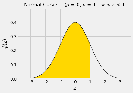
The numerical value of the shaded area can be found by calling stats.norm.cdf.

Python

stats.norm.cdf(1)
# 0.8413447460685429

That’s about 84%. We can now use the symmetry of the curve and the fact that the total area under the curve is 1 to find other areas.

The area to the right of $z=1$ is about 100% - 84% = 16%.

Python

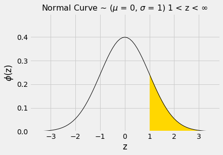
1 - stats.norm.cdf(1)
# 0.15865525393145707

The area between $z=−1$ and $z=1$ can be computed in several different ways. It is the gold area under the curve below.

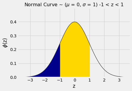
For example, we could calculate the area as “100% - two equal tails”, which works out to roughly 100% - 2x16% = 68%.

Or we could note that the area between $z=1$ and $z=−1$ is equal to all the area to the left of $z=1$, minus all the area to the left of $z=−1$.

Python

stats.norm.cdf(1) - stats.norm.cdf(-1)
# 0.6826894921370859

By a similar calculation, we see that the area between In other words, if a histogram is roughly bell shaped, the proportion of data in the range “average $\pm$ 2 SDs” is about 95%.

That is quite a bit more than Chebyshev’s lower bound of 75%. Chebyshev’s bound is weaker because it has to work for all distributions. If we know that a distribution is normal, we have good approximations to the proportions, not just bounds.

The table below compares what we know about all distributions and about normal distributions. Notice that when 𝑧=1, Chebyshev’s bound is correct but not illuminating.−2 and 2 is about 95%.

Percent in Range	All Distributions: Bound	Normal Distribution: Approximation
average $\pm$ 1 SD	at least 0%	about 68%
average $\pm$ 2 SDs	at least 75%	about 95%
average $\pm$ 3 SDs	at least 88.888…%	about 99.73%

---

The Central Limit Theorem

Very few of the data histograms that we have seen in this course have been bell shaped. When we have come across a bell shaped distribution, it has almost invariably been an empirical histogram of a statistic based on a random sample.

The examples below show two very different situations in which an approximate bell shape appears in such histograms.

---

Net Gain in Roulette

In an earlier section, the bell appeared as the rough shape of the total amount of money we would make if we placed the same bet repeatedly on different spins of a roulette wheel.

Python

# Import dataset roulette_wheel.csv
wheel = pd.read_csv('https://github.com/ZacksAmber/Code/raw/master/Data%20Science/Data8/Data%20Sets/roulette_wheel.csv')
wheel

	Pocket	Color
0	0	green
1	0	green
2	1	red
3	2	black
4	3	red
...	...	...
33	32	red
34	33	black
35	34	red
36	35	black
37	36	red

Recall that the bet on red pays even money, 1 to 1. We defined the function red_winnings that returns the net winnings on one $1 bet on red. Specifically, the function takes a color as its argument and returns 1 if the color is red. For all other colors it returns -1.

Python

# Define function red_winnings for filtering red wheel
def red_winnings(color):
    if color == 'red':
        return 1
    else:
        return -1

The table red shows each pocket’s winnings on red.

Python

# Apply function red_winnings
red = wheel.copy()
red['Winnings: Red'] = red.Color.apply(red_winnings)

red

	Pocket	Color	Winnings: Red
0	0	green	-1
1	0	green	-1
2	1	red	1
3	2	black	-1
4	3	red	1
...	...	...	...
33	32	red	1
34	33	black	-1
35	34	red	1
36	35	black	-1
37	36	red	1

Your net gain on one bet is one random draw from the Winnings: Red column. There is an 18/38 chance making USD 1, and a 20/38 chance of making USD -1. This probability distribution is shown in the histogram below.

Python

# Histogram of Winnings: Red
fig = px.histogram(red, 
                   histnorm='percent', 
                   x='Winnings: Red', 
                   color_discrete_sequence=['rgb(71, 92, 118)'], 
                   opacity=0.9)
# Set bins
fig.update_traces(xbins=dict(start=-1.5, end=1.6, size=1))
# Set layout
fig.update_layout(title='Histogram of Winnings: Red', 
                  yaxis_title='Percent')

fig.show()
# fig.write_image('fig.svg')
# ![](https://raw.githubusercontent.com/ZacksAmber/PicGo/master/img/20210419193649.svg)

Now suppose you bet many times on red. Your net winnings will be the sum of many draws made at random with replacement from the distribution above.

It will take a bit of math to list all the possible values of your net winnings along with all of their chances. We won’t do that; instead, we will approximate the probability distribution by simulation, as we have done all along in this course.

The code below simulates your net gain if you bet USD 1 on red on 400 different spins of the roulette wheel.

Python

# Simulation
num_bets = 400
repetitions = 10000

net_gain_red = np.array([])

# Sumulate 10,000 times
for i in np.arange(repetitions):
    # Generate one value
    spins = red.sample(n=400, replace=True).reset_index(drop=True)
    new_net_gain_red = spins['Winnings: Red'].sum()
    # Add one value to results
    net_gain_red = np.append(net_gain_red, new_net_gain_red)


results = pd.DataFrame({'Net Gain on Red': net_gain_red})

results

	Net Gain on Red
0	-4.0
1	8.0
2	-14.0
3	-52.0
4	-22.0
...	...
9995	0.0
9996	-20.0
9997	2.0
9998	-14.0
9999	2.0

Python

# Histogram of Net Gain on Red
fig = px.histogram(results, 
                   histnorm='percent', 
                   x='Net Gain on Red', 
                   color_discrete_sequence=['rgb(71, 92, 118)'], 
                   opacity=0.9)
# Set bins
fig.update_traces(xbins=dict(start=-80, end=50, size=6))
# Set layout
fig.update_layout(title='Histogram of Net Gain on Red', 
                  yaxis_title='Percent')

fig.show()
# fig.write_image('fig.svg')
# ![](https://raw.githubusercontent.com/ZacksAmber/PicGo/master/img/20210419200246.svg)

That’s a roughly bell shaped histogram, even though the distribution we are drawing from is nowhere near bell shaped.

Center. The distribution is centered near -20 dollars, roughly. To see why, note that your winnings will be USD 1 on about 18/38 of the bets, and USD -1 on the remaining 20/38. So your average winnings per dollar bet will be roughly -5.26 cents:

Python

# Probability of Winning on Red
len(red[red.Color == 'red'])
print(f"Probability of Winning on Red is {len(red[red.Color == 'red'])} / {len(red)} == {round(len(red[red.Color == 'red'])/len(red), 2)}")
# Probability of Winning on Red is 18 / 38 == 0.47

Python

# Expected Value
average_per_bet = 1*(18/38) + (-1)*(20/38)
average_per_bet
# -0.05263157894736842

So in 400 bets you expect that your net gain will be about USD -21:

Python

# Expected Value of 400 bets
average_per_bet * 400
# -21.052631578947366

For confirmation, we can compute the mean of the 10,000 simulated net gains:

Python

# Mean
np.mean(results['Net Gain on Red'])
# -21.0104

Spread. Run your eye along the curve starting at the center and notice that the point of inflection is near 0. On a bell shaped curve, the SD is the distance from the center to a point of inflection. The center is roughly USD -20, which means that the SD of the distribution is around USD 20.

In the next section we will see where the USD 20 comes from. For now, let’s confirm our observation by simply calculating the SD of the 10,000 simulated net gains:

Python

# Standard Deviation
np.std(results['Net Gain on Red'])
# 20.09801711214318

Summary. The net gain in 400 bets is the sum of the 400 amounts won on each individual bet. The probability distribution of that sum is approximately normal, with an average and an SD that we can approximate.

---

Average Flight Delay

The table united contains data on departure delays of 13,825 United Airlines domestic flights out of San Francisco airport in the summer of 2015. As we have seen before, the distribution of delays has a long right-hand tail.

Python

# Import dataset united_summer2015.csv
united = pd.read_csv('https://github.com/ZacksAmber/Code/raw/master/Data%20Science/Data8/Data%20Sets/united_summer2015.csv')

united

	Date	Flight Number	Destination	Delay
0	6/1/15	73	HNL	257
1	6/1/15	217	EWR	28
2	6/1/15	237	STL	-3
3	6/1/15	250	SAN	0
4	6/1/15	267	PHL	64
...	...	...	...	...
13820	8/31/15	1978	LAS	-4
13821	8/31/15	1993	IAD	8
13822	8/31/15	1994	ORD	3
13823	8/31/15	2000	PHX	-1
13824	8/31/15	2013	EWR	-2

Python

# Histogram of Delay
fig = px.histogram(united, 
                   histnorm='percent', 
                   x='Delay', 
                   color_discrete_sequence=['rgb(71, 92, 118)'], 
                   opacity=0.9)
# Set bins
fig.update_traces(xbins=dict(start=-20, end=300, size=10))
# Set layout
fig.update_layout(title='Histogram of Delay', 
                  yaxis_title='Percent')

fig.show()
# fig.write_image('fig.svg')
# ![](https://raw.githubusercontent.com/ZacksAmber/PicGo/master/img/20210419204343.svg)

The mean delay was about 16.6 minutes and the SD was about 39.5 minutes. Notice how large the SD is, compared to the mean. Those large deviations on the right have an effect, even though they are a very small proportion of the data.

Python

# Mean and SD of Delay
mean_delay = np.mean(united.Delay)
sd_delay = np.std(united.Delay)

mean_delay, sd_delay
# (16.658155515370705, 39.480199851609314)

Python

len(united)
# 13825

Now suppose we sampled 400 delays at random with replacement. You could sample without replacement if you like, but the results would be very similar to with-replacement sampling. If you sample a few hundred out of 13,825 without replacement, you hardly change the population each time you pull out a value.

In the sample, what could the average delay be? We expect it to be around 16 or 17, because that’s the population average; but it is likely to be somewhat off. Let’s see what we get by sampling. We’ll work with the table delay that only contains the column of delays.

Python

# Extract column Delay from united
delay = united.Delay

Python

# Generate one value
np.mean(delay.sample(n=400, replace=True, random_state=2021))
# 16.295

The sample average varies according to how the sample comes out, so we will simulate the sampling process repeatedly and draw the empirical histogram of the sample average. That will be an approximation to the probability histogram of the sample average.

Python

# Simulation
sample_size = 400
repetitions = 10000

means = np.array([])

for i in np.arange(repetitions):
    # Generate one value
    sample = delay.sample(n=sample_size, replace=True)
    new_mean = np.mean(sample)
    # Add one value to results
    means = np.append(means, new_mean)

results = pd.DataFrame({'Sample Mean': means})

Python

results

	Sample Mean
0	17.7275
1	19.7425
2	16.8400
3	16.6075
4	13.2800
...	...
9995	15.2075
9996	18.2050
9997	15.4025
9998	16.0925
9999	14.7000

Python

# Histogram of Sample Mean from United
fig = px.histogram(results, 
                   histnorm='percent', 
                   x='Sample Mean', 
                   color_discrete_sequence=['rgb(71, 92, 118)'], 
                   opacity=0.9)
# Set bins
fig.update_traces(xbins=dict(start=10, end=25, size=0.5))
# Set layout
fig.update_layout(title='Histogram of Sample Mean from United', 
                  yaxis_title='Percent')

fig.show()
# fig.write_image('fig.svg')
# ![](https://raw.githubusercontent.com/ZacksAmber/PicGo/master/img/20210419210155.svg)

Once again, we see a rough bell shape, even though we are drawing from a very skewed distribution. The bell is centered somewhere between 16 and 17, as we expect.

Python

# Mean
np.mean(results['Sample Mean'])
# 16.64065875

Python

# SD
np.std(results['Sample Mean'])
# 1.9665278355323215

---

Central Limit Theorem

The reason why the bell shape appears in such settings is a remarkable result of probability theory called the Central Limit Theorem.

The Central Limit Theorem says that the probability distribution of the sum or average of a large random sample drawn with replacement will be roughly normal, regardless of the distribution of the population from which the sample is drawn.

As we noted when we were studying Chebyshev’s bounds, results that can be applied to random samples regardless of the distribution of the population are very powerful, because in data science we rarely know the distribution of the population.

The Central Limit Theorem makes it possible to make inferences with very little knowledge about the population, provided we have a large random sample. That is why it is central to the field of statistical inference.

---

Proportion of Purple Flowers

Recall Mendel’s probability model for the colors of the flowers of a species of pea plant. The model says that the flower colors of the plants are like draws made at random with replacement from {Purple, Purple, Purple, White}.

In a large sample of plants, about what proportion will have purple flowers? We would expect the answer to be about 0.75, the proportion purple in the model. And, because proportions are means, the Central Limit Theorem says that the distribution of the sample proportion of purple plants is roughly normal.

We can confirm this by simulation. Let’s simulate the proportion of purple-flowered plants in a sample of 200 plants.

Python

# Make DataFrame model
colors = np.array(['Purple', 'Purple', 'Purple', 'White'])

model = pd.DataFrame({'Color': colors})

model

	Color
0	Purple
1	Purple
2	Purple
3	White

Python

# Simulation
props = np.array([])

num_plants = 200
repetitions = 10000

for i in np.arange(repetitions):
    # Generate one value
    sample = model.sample(n=num_plants, replace=True)
    new_prop = np.count_nonzero(sample[sample.Color == 'Purple'])/num_plants
    # Add one value to props
    props = np.append(props, new_prop)

# Store props in DataFrame
results = pd.DataFrame({'Sample Proportion: 200': props})

Python

results

	Sample Proportion: 200
0	0.760
1	0.725
2	0.770
3	0.735
4	0.760
...	...
9995	0.780
9996	0.750
9997	0.790
9998	0.705
9999	0.745

Python

# Histogram of Sample Proportion: 200 from model
fig = px.histogram(results, 
                   histnorm='percent', 
                   x='Sample Proportion: 200', 
                   color_discrete_sequence=['rgb(71, 92, 118)'], 
                   opacity=0.9)
# Set bins
fig.update_traces(xbins=dict(start=0.65, end=0.85, size=0.01))
# Set layout
fig.update_layout(title='Histogram of Sample Proportion: 200 from model', 
                  yaxis_title='Percent')

fig.show()
# fig.write_image('fig.svg')
# ![](https://raw.githubusercontent.com/ZacksAmber/PicGo/master/img/20210419213509.svg)

There’s that normal curve again, as predicted by the Central Limit Theorem, centered at around 0.75 just as you would expect.

How would this distribution change if we increased the sample size? Let’s run the code again with a sample size of 800, and collect the results of simulations in the same table in which we collected simulations based on a sample size of 200. We will keep the number of repetitions the same as before so that the two columns have the same length.

Python

# Simulation Again
props2 = np.array([])

num_plants = 800

for i in np.arange(repetitions):
    # Generate one value
    sample = model.sample(n=num_plants, replace=True)
    new_prop = np.count_nonzero(sample[sample.Color == 'Purple'])/num_plants
    # Add one value to props
    props2 = np.append(props2, new_prop)

# Add props2 in DataFrame
results['Sample Proportion: 800'] = props2

Python

results

	Sample Proportion: 200	Sample Proportion: 800
0	0.760	0.77625
1	0.725	0.76250
2	0.770	0.76000
3	0.735	0.74500
4	0.760	0.76125
...	...	...
9995	0.780	0.75250
9996	0.750	0.77625
9997	0.790	0.77125
9998	0.705	0.74750
9999	0.745	0.75875

Python

# Histogram of Sample Proportion: 800 from model
fig = px.histogram(results, 
                   histnorm='percent', 
                   x='Sample Proportion: 800', 
                   color_discrete_sequence=['rgb(71, 92, 118)'], 
                   opacity=0.9)
# Set bins
fig.update_traces(xbins=dict(start=0.65, end=0.85, size=0.01))
# Set layout
fig.update_layout(title='Histogram of Sample Proportion: 800 from model', 
                  yaxis_title='Percent')

fig.show()
# fig.write_image('fig.svg')
# ![](https://raw.githubusercontent.com/ZacksAmber/PicGo/master/img/20210419213620.svg)

Python

# Overlaid Histogram of Sample Proportion: 200 and Sample Proportion: 800 from model
# Histogram of Sample Proportion: 800 from model
fig = px.histogram(results, 
                   histnorm='percent', 
                   barmode='overlay', 
                   x=['Sample Proportion: 200', 'Sample Proportion: 800'], 
                   color_discrete_sequence=['rgb(71, 92, 118)', 'rgb(250, 211, 102)'], 
                   opacity=0.9)
# Set bins
fig.update_traces(xbins=dict(start=0.65, end=0.85, size=0.01))
# Set layout
fig.update_layout(title='Histogram of Sample Proportion: 200 and Sample Proportion: 800 from model', 
                  yaxis_title='Percent')

fig.show()
# fig.write_image('fig.svg')
# ![](https://raw.githubusercontent.com/ZacksAmber/PicGo/master/img/20210419213620.svg)

Both distributions are approximately normal but one is narrower than the other. The proportions based on a sample size of 800 are more tightly clustered around 0.75 than those from a sample size of 200. Increasing the sample size has decreased the variability in the sample proportion.

This should not be surprising. We have leaned many times on the intuition that a larger sample size generally reduces the variability of a statistic. However, in the case of a sample average, we can quantify the relationship between sample size and variability.

Exactly how does the sample size affect the variability of a sample average or proportion? That is the question we will examine in the next section.

---

The Variability of the Sample Mean

By the Central Limit Theorem, the probability distribution of the mean of a large random sample is roughly normal. The bell curve is centered at the population mean. Some of the sample means are higher, and some lower, but the deviations from the population mean are roughly symmetric on either side, as we have seen repeatedly. Formally, probability theory shows that the sample mean is an unbiased estimate of the population mean.

In our simulations, we also noticed that the means of larger samples tend to be more tightly clustered around the population mean than means of smaller samples. In this section, we will quantify the variability of the sample mean and develop a relation between the variability and the sample size.

Let’s start with our table of flight delays. The mean delay is about 16.7 minutes, and the distribution of delays is skewed to the right.

Python

# Import dataset united_summer2015.csv
united = pd.read_csv('https://github.com/ZacksAmber/Code/raw/master/Data%20Science/Data8/Data%20Sets/united_summer2015.csv')

united

	Date	Flight Number	Destination	Delay
0	6/1/15	73	HNL	257
1	6/1/15	217	EWR	28
2	6/1/15	237	STL	-3
3	6/1/15	250	SAN	0
4	6/1/15	267	PHL	64
...	...	...	...	...
13820	8/31/15	1978	LAS	-4
13821	8/31/15	1993	IAD	8
13822	8/31/15	1994	ORD	3
13823	8/31/15	2000	PHX	-1
13824	8/31/15	2013	EWR	-2

Python

# Extract Delay from united
delay = united.loc[:, ['Delay']]

# Mean of population
pop_mean = np.mean(delay.Delay)
pop_mean
# 16.658155515370705

Python

# Histogram of Delay: Population
fig = px.histogram(delay, 
                   histnorm='percent', 
                   x='Delay', 
                   color_discrete_sequence=['rgb(71, 92, 118)'], 
                   opacity=0.9)
# Set bins
fig.update_traces(xbins=dict(start=-20, end=301, size=10))
# Set layout
fig.update_layout(title='Histogram of Delay: Population', 
                  yaxis_title='Percent'
)
# Add marker to fig
fig.add_trace(
    go.Scatter(
        mode='markers', 
        marker_symbol='triangle-up', 
        x=[np.mean(delay.Delay)],
        y=[-1],
        marker=dict(
            color='rgb(0, 0, 139)',
            size=8,
        ),
        showlegend=False
    )
)

fig.show()
# fig.write_image('fig.svg')
# ![](https://raw.githubusercontent.com/ZacksAmber/PicGo/master/img/20210420004024.svg)

Now let’s take random samples and look at the probability distribution of the sample mean. As usual, we will use simulation to get an empirical approximation to this distribution.

We will define a function simulate_sample_mean to do this, because we are going to vary the sample size later. The arguments are the name of the table, the label of the column containing the variable, the sample size, and the number of simulations.

Python

"""Empirical distribution of random sample means"""

def simulate_sample_mean(table, label, sample_size, repetitions):
    # Make an array mean for storing sample means
    means = np.array([])

    for i in range(repetitions):
        new_sample = table.sample(n=sample_size, replace=False).reset_index(drop=True)
        new_sample_mean = np.mean(new_sample[label])
        means = np.append(means, new_sample_mean)
    
    # Store means in DataFrame sample_means
    sample_means = pd.DataFrame({'Sample Means': means})
    
    # Display empirical histogram and print all relevant quantities
    # Histogram of Delay: Sample
    fig = px.histogram(sample_means, 
                       histnorm='percent', 
                       x='Sample Means', 
                       range_x=[5, 35], 
                       range_y=[0, 25], 
                       nbins=20, 
                       color_discrete_sequence=['rgb(71, 92, 118)'], 
                       opacity=0.9)
    # Set layout
    fig.update_layout(title=f'Histogram of Delay: Sample, Sample Size {str(sample_size)}', 
                      yaxis_title='Percent')


    fig.show()
    fig.write_image('fig.svg')
       
    print("Sample size: ", sample_size)
    print("Population mean:", np.mean(table[label]))
    print("Average of sample means: ", np.mean(means))
    print("Population SD:", np.std(table[label]))
    print("SD of sample means:", np.std(means))

Let us simulate the mean of a random sample of 100 delays, then of 400 delays, and finally of 625 delays. We will perform 10,000 repetitions of each of these process. The range_x and range_y lines set the axes consistently in all the plots for ease of comparison.

Python

simulate_sample_mean(delay, 'Delay', 100, 10000)
# ![](https://raw.githubusercontent.com/ZacksAmber/PicGo/master/img/20210420004735.svg)

Python

Sample size:  100
Population mean: 16.658155515370705
Average of sample means:  16.739301
Population SD: 39.480199851609314
SD of sample means: 3.9528995764374026

Python

simulate_sample_mean(delay, 'Delay', 400, 10000)
# ![](https://raw.githubusercontent.com/ZacksAmber/PicGo/master/img/20210420004826.svg)

Python

Sample size:  400
Population mean: 16.658155515370705
Average of sample means:  16.654101999999998
Population SD: 39.480199851609314
SD of sample means: 1.9286672606611022

Python

simulate_sample_mean(delay, 'Delay', 625, 10000)
# ![](https://raw.githubusercontent.com/ZacksAmber/PicGo/master/img/20210420004917.svg)

Python

Sample size:  625
Population mean: 16.658155515370705
Average of sample means:  16.6409256
Population SD: 39.480199851609314
SD of sample means: 1.54393821773821

You can see the Central Limit Theorem in action – the histograms of the sample means are roughly normal, even though the histogram of the delays themselves is far from normal.

You can also see that each of the three histograms of the sample means is centered very close to the population mean. In each case, the “average of sample means” is very close to 16.66 minutes, the population mean. Both values are provided in the printout above each histogram. As expected, the sample mean is an unbiased estimate of the population mean.

---

The SD of All the Sample Means

You can also see that the histograms get narrower, and hence taller, as the sample size increases. We have seen that before, but now we will pay closer attention to the measure of spread.

The SD of the population of all delays is about 40 minutes.

Python

# SD of Delay
pop_sd = np.std(delay['Delay'])
pop_sd
# 39.480199851609314

Take a look at the SDs in the sample mean histograms above. In all three of them, the SD of the population of delays is about 40 minutes, because all the samples were taken from the same population.

Now look at the SD of all 10,000 sample means, when the sample size is 100. That SD is about one-tenth of the population SD. When the sample size is 400, the SD of all the sample means is about one-twentieth of the population SD. When the sample size is 625, the SD of the sample means is about one-twentyfifth of the population SD.

It seems like a good idea to compare the SD of the empirical distribution of the sample means to the quantity “population SD divided by the square root of the sample size.”

Here are the numerical values. For each sample size in the first column, 10,000 random samples of that size were drawn, and the 10,000 sample means were calculated. The second column contains the SD of those 10,000 sample means. The third column contains the result of the calculation “population SD divided by the square root of the sample size.”

The cell takes a while to run, as it’s a large simulation. But you’ll soon see that it’s worth the wait.

Python

# Repeat Simulation in different sample sizes
repetitions = 10000
sample_sizes = np.arange(25, 626, 25)

# Create array sd_means for storing 25 times Simulations
sd_means = np.array([])

for n in sample_sizes:
    # Create array means for storing means from simulation
    means = np.array([])
    # Simulation
    for i in np.arange(repetitions): 
        # Generate one value
        means = np.append(means, np.mean(delay.sample(n=n, replace=False).reset_index(drop=True)['Delay']))
    # Calculate the SD of 10,000 means then store it in sd_means
    sd_means = np.append(sd_means, np.std(means))

# Creata DataFrame sd_comparison for storing sd_means and pop_sd/sqrt(n)
sd_comparison = pd.DataFrame({
    'Sample Size n': sample_sizes,
    'SD of 10,000 Sample Means': sd_means,
    'pop_sd/sqrt(n)': pop_sd/np.sqrt(sample_sizes)
})

Python

sd_comparison

	Sample Size n	SD of 10,000 Sample Means	pop_sd/sqrt(n)
0	25	7.921527	7.896040
1	50	5.580221	5.583343
2	75	4.543732	4.558781
3	100	3.965510	3.948020
4	125	3.500722	3.531216
...	...	...	...
20	525	1.663286	1.723057
21	550	1.644531	1.683441
22	575	1.596109	1.646438
23	600	1.567117	1.611772
24	625	1.518364	1.579208

The values in the second and third columns are very close. If we plot each of those columns with the sample size on the horizontal axis, the two graphs are essentially indistinguishable.

Python

# Line Chart
fig = px.line(sd_comparison, 
              x='Sample Size n', 
              y=['SD of 10,000 Sample Means', 'pop_sd/sqrt(n)'], 
              color_discrete_sequence=['rgb(71, 92, 118)', 'rgb(250, 211, 102)'])
# Set layout
fig.update_layout(yaxis_title='')

fig.show()
# fig.write_image('fig.svg')
# ![](https://raw.githubusercontent.com/ZacksAmber/PicGo/master/img/20210420013128.svg)

There really are two curves there. But they are so close to each other that it looks as though there is just one.

What we are seeing is an instance of a general result. Remember that the graph above is based on 10,000 replications for each sample size. But there are many more than 10,000 samples of each size. The probability distribution of the sample mean is based on the means of all possible samples of a fixed size.

Fix a sample size. If the samples are drawn at random with replacement from the population, then

$${\mbox{SD of all possible sample means}} =
\frac{\mbox{Population SD}}{\sqrt{\mbox{sample size}}}$$

$$\mbox{Standard Error}: SE = \frac{\sigma}{\sqrt{n}}$$

This is the standard deviation of the averages of all the possible samples that could be drawn. It measures roughly how far off the sample means are from the population mean.

---

The Central Limit Theorem for the Sample Mean

If you draw a large random sample with replacement from a population, then, regardless of the distribution of the population, the probability distribution of the sample mean is roughly normal, centered at the population mean, with an SD equal to the population SD divided by the square root of the sample size.

---

The Accuracy of the Sample Mean

The SD of all possible sample means measures how variable the sample mean can be. As such, it is taken as a measure of the accuracy of the sample mean as an estimate of the population mean. The smaller the SD, the more accurate the estimate.

The formula shows that:

• The population size doesn’t affect the accuracy of the sample mean. The population size doesn’t appear anywhere in the formula.
• The population SD is a constant; it’s the same for every sample drawn from the population. The sample size can be varied. Because the sample size appears in the denominator, the variability of the sample mean decreases as the sample size increases, and hence the accuracy increases.

---

The Square Root Law

From the table of SD comparisons, you can see that the SD of the means of random samples of 25 flight delays is about 8 minutes. If you multiply the sample size by 4, you’ll get samples of size 100. The SD of the means of all of those samples is about 4 minutes. That’s smaller than 8 minutes, but it’s not 4 times as small; it’s only 2 times as small. That’s because the sample size in the denominator has a square root over it. The sample size increased by a factor of 4, but the SD went down by a factor of $2=\sqrt{4}$. In other words, the accuracy went up by a factor of $2=\sqrt{4}$.

In general, when you multiply the sample size by a factor, the accuracy of the sample mean goes up by the square root of that factor.

So to increase accuracy by a factor of 10, you have to multiply sample size by a factor of 100. Accuracy doesn’t come cheap!

---

Choosing a Sample Size

Candidate A is contesting an election. A polling organization wants to estimate the proportion of voters who will vote for her. Let’s suppose that they plan to take a simple random sample of voters, though in reality their method of sampling would be more complex. How can they decide how large their sample should be, to get a desired level of accuracy?

We are now in a position to answer this question, after making a few assumptions:

• The population of voters is very large and that therefore we can just as well assume that the random sample will be drawn with replacement.
• The polling organization will make its estimate by constructing an approximate 95% confidence interval for the percent of voters who will vote for Candidate A.
• The desired level of accuracy is that the width of the interval should be no more than 1%. That’s pretty accurate! For example, the confidence interval (33.2%, 34%) would be fine but (33.2%, 35%) would not.

We will work with the sample proportion of voters for Candidate A. Recall that a proportion is a mean, when the values in the population are only 0 (the type of individual you are not counting) or 1 (the type of individual you are counting).

---

Width of Confidence Interval

If we had a random sample, we could go about using the bootstrap to construct a confidence interval for the percent of voters for Candidate A. But we don’t have a sample yet – we are trying to find out how big the sample has to be so that our confidence interval is as narrow as we want it to be.

In situations like this, it helps to see what theory predicts.

The Central Limit Theorem says that the probabilities for the sample proportion are roughly normally distributed, centered at the population proportion of 1’s, with an SD equal to the SD of the population of 0’s and 1’s divided by the square root of the sample size.

So the confidence interval will still be the “middle 95%” of a normal distribution, even though we can’t pick off the ends as the 2.5th and 97.5th percentiles of bootstrapped proportions.

Is there another way to find how wide the interval would be? Yes, because we know that for normally distributed variables, the interval “center ± 2 SDs” contains 95% of the data.

The confidence interval will stretch for 2 SDs of the sample proportion, on either side of the center. So the width of the interval will be 4 SDs of the sample proportion.

We are willing to tolerate a width of 1% = 0.01. So, using the formula developed in the last section,

Python

stats.norm.cdf(0-2)
# 0.022750131948179195

Python

stats.norm.cdf(0+2)
# 0.9772498680518208

$$4 \times \frac{\mbox{SD of the 0-1 population}}{\sqrt{\mbox{sample size}}} \le ~ 0.01$$

So

$$\sqrt{\mbox{sample size}} \ge 4 \times \frac{\mbox{SD of the 0-1 population}}{0.01}$$

---

The SD of a collection of 0’s and 1’s

If we knew the SD of the population, we’d be done. We could calculate the square root of the sample size, and then take the square to get the sample size. But we don’t know the SD of the population. The population consists of 1 for each voter for Candidate A, and 0 for all other voters, and we don’t know what proportion of each kind there are. That’s what we’re trying to estimate.

So are we stuck? No, because we can bound the SD of the population. Here are histograms of two such distributions, one for an equal proportion of 1’s and 0’s, and one with 90% 1’s and 10% 0’s. Which one has the bigger SD?

Python

# Probability of the proportion of True:False with 9:1, and 5:5
prob = pd.DataFrame({"Proportion of 1's: 0.9": [0] + [1] * 9, 
                     "Proportion of 1's: 0.5": [0] * 5 + [1] * 5})
prob

	Proportion of 1's: 0.9	Proportion of 1's: 0.5
0	0	0
1	1	0
2	1	0
3	1	0
4	1	0
5	1	1
6	1	1
7	1	1
8	1	1
9	1	1

Python

# Histogram of The SD of a collection of 0’s and 1’s
fig = px.histogram(prob, 
                   histnorm='percent', 
                   x=["Proportion of 1's: 0.5", "Proportion of 1's: 0.9"], 
                   range_y=[0, 100], 
                   barmode='overlay', 
                   color_discrete_sequence=['rgb(71, 92, 118)', 'rgb(250, 211, 102)'], 
                   opacity=0.9)
# Set bins
fig.update_traces(xbins=dict(start=-0.5, end=1.5, size=1))
# Set layout
fig.update_layout(title='The SD of a collection of 0’s and 1’s', 
                  xaxis_title='', # remove xaxis_titile
                  yaxis_title='Percent'
)
# Add marker to fig
fig.add_trace(
    go.Scatter(
        mode='markers', 
        marker_symbol='triangle-up', 
        x=[0.5],
        y=[-1],
        marker=dict(
            color='rgb(0, 0, 139)',
            size=8,
        ),
        showlegend=False
    )
)

fig.show()
# fig.write_image('fig.svg')
# ![](https://raw.githubusercontent.com/ZacksAmber/PicGo/master/img/20210420204038.svg)

Remember that the possible values in the population are only 0 and 1.

The blue histogram (50% 1’s and 50% 0’s) has more spread than the gold. The mean is 0.5. Half the deviations from mean are equal to 0.5 and the other half equal to -0.5, so the SD is 0.5.

In the gold histogram, all of the area is being squished up around 1, leading to less spread. 90% of the deviations are small: 0.1. The other 10% are -0.9 which is large, but overall the spread is smaller than in the blue histogram.

The same observation would hold if we varied the proportion of 1’s or let the proportion of 0’s be larger than the proportion of 1’s. Let’s check this by calculating the SDs of populations of 10 elements that only consist of 0’s and 1’s, in varying proportions. The function np.ones is useful for this. It takes a positive integer as its argument and returns an array consisting of that many 1’s.

numpy.ones

Python

# Generate Population SD of different proportions
sd = np.array([])
for i in np.arange(1, 10, 1):
    # Create an array of i 1's and (10-i) 0's
    population = np.append(np.ones(i), 1-np.ones(10-i))
    sd = np.append(sd, np.std(population))
    
zero_one_sds = pd.DataFrame({
    "Population Proportion of 1's": np.arange(0.1, 1, 0.1),
    "Population SD": sd
})

zero_one_sds

	Population Proportion of 1's	Population SD
0	0.1	0.300000
1	0.2	0.400000
2	0.3	0.458258
3	0.4	0.489898
4	0.5	0.500000
5	0.6	0.489898
6	0.7	0.458258
7	0.8	0.400000
8	0.9	0.300000

Not surprisingly, the SD of a population with 10% 1’s and 90% 0’s is the same as that of a population with 90% 1’s and 10% 0’s. That’s because you switch the bars of one histogram to get the other; there is no change in spread.

More importantly for our purposes, the SD increases as the proportion of 1’s increases, until the proportion of 1’s is 0.5; then it starts to decrease symmetrically.

Python

# Scatter of zero_one_sds
fig = px.scatter(zero_one_sds, 
                 x="Population Proportion of 1's", 
                 y='Population SD')

fig.show()
# fig.write_image('fig.svg')
# ![](https://raw.githubusercontent.com/ZacksAmber/PicGo/master/img/20210420205305.svg)

Summary: The SD of a population of 1’s and 0’s is at most 0.5. That’s the value of the SD when 50% of the population is coded 1 and the other 50% are coded 0.

---

The Sample Size

We know that

$$\sqrt{\mbox{sample size}} \ge 4 \times \frac{\mbox{SD of the 0-1 population}}{0.01}$$

and that the SD of the 0-1 population is at most 0.5, regardless of the proportion of 1’s in the population. So it is safe to take

$$\sqrt{\mbox{sample size}} \ge 4 \times \frac{0.5}{0.01} = 200$$

So the sample size should be at least $200^2=40,000$. That’s an enormous sample! But that’s what you need if you want to guarantee great accuracy with high confidence no matter what the population looks like.

---

Prediction

Prediction
Program: Data8-15.ipynb
Program: Data8-15-2.ipynb

An important aspect of data science is to find out what data can tell us about the future. What do data about climate and pollution say about temperatures a few decades from now? Based on a person’s internet profile, which websites are likely to interest them? How can a patient’s medical history be used to judge how well he or she will respond to a treatment?

To answer such questions, data scientists have developed methods for making predictions. In this chapter we will study one of the most commonly used ways of predicting the value of one variable based on the value of another.

Here is a historical dataset used for the prediction of the heights of adults based on the heights of their parents. We have studied this dataset in an earlier section. The table heights contains data on the midparent height and child’s height (all in inches) for a population of 934 adult “children”. Recall that the midparent height is an average of the heights of the two parents.

Python

# Import dataset galton.csv
# Data on heights of parents and their adult children
original = pd.read_csv('https://github.com/ZacksAmber/Code/raw/master/Data%20Science/Data8/Data%20Sets/galton.csv')
heights = pd.DataFrame({
    'MidParent': original['midparentHeight'],
    'Child': original['childHeight']
})

heights

MidParent	Child
75.43	73.2
75.43	69.2
75.43	69
75.43	69
73.66	73.5
73.66	72.5
73.66	65.5
73.66	65.5
72.06	71
72.06	68

Python

# Scatter of Child vs. MidParent
fig = px.scatter(heights, 
                 x='MidParent', 
                 y='Child', 
                 color_discrete_sequence=['rgb(2, 21 ,51)'], 
                 opacity=0.7)
# Set layout
fig.update_layout(title='Scatter of Child vs. MidParent')

fig.show()
# fig.write_image('fig.svg')
# ![](https://raw.githubusercontent.com/ZacksAmber/PicGo/master/img/20210421225052.svg)

A primary reason for studying the data was to be able to predict the adult height of a child born to parents who were similar to those in the dataset. We made these predictions in Section 8.1, after noticing the positive association between the two variables.

Our approach was to base the prediction on all the points that correspond to a midparent height of around the midparent height of the new person. To do this, we wrote a function called predict_child which takes a midparent height as its argument and returns the average height of all the children who had midparent heights within half an inch of the argument.

Python

# Define predict_child for predicting any value of the midparent height
def predict_child(mpht):
    """Predict the height of a child whose parents have a midparent height of mpht.
    
    The prediction is the average height of the children whose midparent height is
    in the range mpht plus or minus 0.5.
    """
    filter = (mpht-0.5 <= heights.MidParent) & (heights.MidParent <= mpht+0.5)
    close_points = heights.loc[filter]
    
    return np.mean(close_points.Child)

We applied the function to the column of Midparent heights, and visualized the result.

Python

# Apply predict_child to all the midparent heights
heights_with_predictions = heights.copy()
heights_with_predictions['Prediction'] = heights.MidParent.apply(predict_child)
heights_with_predictions

	MidParent	Child	Prediction
0	75.43	73.2	70.100000
1	75.43	69.2	70.100000
2	75.43	69.0	70.100000
3	75.43	69.0	70.100000
4	73.66	73.5	70.415789
...	...	...	...
929	66.64	64.0	65.156579
930	66.64	62.0	65.156579
931	66.64	61.0	65.156579
932	65.27	66.5	64.229630
933	65.27	57.0	64.229630

Python

# Apply predict_child to all the midparent heights
heights_with_predictions = heights.copy()
heights_with_predictions['Prediction'] = heights.MidParent.apply(predict_child)
heights_with_predictions

Scatter Plots in Python
plotly.graph_objects.Scatter

Python

# Draw the original scatter plot along with the predicted values
fig = go.Figure()

# Add trace Child
fig.add_trace(go.Scatter(
    mode='markers', 
    x=heights_with_predictions['MidParent'], 
    y=heights_with_predictions['Child'], 
    name='Child', 
    marker_color='rgba(2, 21 ,51, .8)')) # rgb + opacity

# Add trace Prediction
fig.add_trace(go.Scatter(
    mode='markers', 
    x=heights_with_predictions['MidParent'], 
    y=heights_with_predictions['Prediction'], 
    name='Predication', 
    marker_color='rgba(250, 211, 102, .8)')) # rgb + opacity

# Set layout
fig.update_layout(title="Prediction of Children's heights", 
                  xaxis_title='MidParent', 
                  yaxis_title='')

fig.show()
# fig.write_image('fig.svg')
# ![](https://raw.githubusercontent.com/ZacksAmber/PicGo/master/img/20210422011901.svg)

The prediction at a given midparent height lies roughly at the center of the vertical strip of points at the given height. This method of prediction is called regression. Later in this chapter we will see whether we can avoid our arbitrary definitions of “closeness” being “within 0.5 inches”. But first we will develop a measure that can be used in many settings to decide how good one variable will be as a predictor of another.

---

Correlation

In this section we will develop a measure of how tightly clustered a scatter diagram is about a straight line. Formally, this is called measuring linear association.

The table hybrid contains data on hybrid passenger cars sold in the United States from 1997 to 2013. The data were adapted from the online data archive of Prof. Larry Winner of the University of Florida. The columns:

• vehicle: model of the car
• year: year of manufacture
• msrp: manufacturer’s suggested retail price in 2013 dollars
• acceleration: acceleration rate in km per hour per second
• mpg: fuel econonmy in miles per gallon
• class: the model’s class.

Python

# Import dataset hybrid.csv
hybrid = pd.read_csv('https://github.com/ZacksAmber/Code/raw/master/Data%20Science/Data8/Data%20Sets/hybrid.csv')
hybrid

	vehicle	year	msrp	acceleration	mpg	class
0	Prius (1st Gen)	1997	24509.74	7.46	41.26	Compact
1	Tino	2000	35354.97	8.20	54.10	Compact
2	Prius (2nd Gen)	2000	26832.25	7.97	45.23	Compact
3	Insight	2000	18936.41	9.52	53.00	Two Seater
4	Civic (1st Gen)	2001	25833.38	7.04	47.04	Compact
...	...	...	...	...	...	...
148	S400	2013	92350.00	13.89	21.00	Large
149	Prius Plug-in	2013	32000.00	9.17	50.00	Midsize
150	C-Max Energi Plug-in	2013	32950.00	11.76	43.00	Midsize
151	Fusion Energi Plug-in	2013	38700.00	11.76	43.00	Midsize
152	Chevrolet Volt	2013	39145.00	11.11	37.00	Compact

The graph below is a scatter plot of msrp versus acceleration. That means msrp is plotted on the vertical axis and accelaration on the horizontal.

Python

# Scatter of msrp vs. acceleration
fig = px.scatter(hybrid, 
                 x='acceleration', 
                 y='msrp', 
                 color_discrete_sequence=['rgb(2, 21 ,51)'], 
                 opacity=0.7)
# Set layout
fig.update_layout(title='Scatter of msrp vs. acceleration')

fig.show()
# fig.write_image('fig.svg')
# ![](https://raw.githubusercontent.com/ZacksAmber/PicGo/master/img/20210422004919.svg)

Notice the positive association. The scatter of points is sloping upwards, indicating that cars with greater acceleration tended to cost more, on average; conversely, the cars that cost more tended to have greater acceleration on average.

The scatter diagram of msrp versus mpg(mileage per gallon) shows a negative association. Hybrid cars with higher mileage tended to cost less, on average. This seems surprising till you consider that cars that accelerate fast tend to be less fuel efficient and have lower mileage. As the previous scatter plot showed, those were also the cars that tended to cost more.

Python

# Scatter of msrp vs. mpg
fig = px.scatter(hybrid, 
                 x='mpg', 
                 y='msrp', 
                 color_discrete_sequence=['rgb(2, 21 ,51)'], 
                 opacity=0.7)
# Set layout
fig.update_layout(title='Scatter of msrp vs. mpg')

fig.show()
# fig.write_image('fig.svg')
# ![](https://raw.githubusercontent.com/ZacksAmber/PicGo/master/img/20210422012735.svg)

Along with the negative association, the scatter diagram of msrp versus mpg shows a non-linear relation between the two variables. The points appear to be clustered around a curve, not around a straight line.

If we restrict the data just to the SUV class, however, the association between msrp and mpg is still negative but the relation appears to be more linear. The relation between the price and acceleration of SUV’s also shows a linear trend, but with a positive slope.

Python

# Extract SUV data from hybrid
suv = hybrid[hybrid['class'] == 'SUV']
suv

	vehicle	year	msrp	acceleration	mpg	class
10	Escape	2004	36676.10	10.32	31.99	SUV
14	Lexus RX400h	2005	58521.14	12.76	28.23	SUV
16	Highlander	2005	29186.21	12.76	29.40	SUV
19	Escape 2WD	2005	19322.56	9.52	29.00	SUV
22	Mercury Mariner	2006	34772.40	8.98	32.93	SUV
...	...	...	...	...	...	...
130	Touareg	2013	62575.00	16.13	21.00	SUV
131	Escalade 2WD	2013	74425.00	11.63	21.00	SUV
132	Tahoe 2WD	2013	53620.00	11.90	21.00	SUV
133	Yukon 1500	2013	54145.00	11.88	21.00	SUV
134	Yukon 1500	2013	61960.00	13.33	21.00	SUV

Python

# Scatter of SUV: msrp vs. mpg
fig = px.scatter(suv, 
                 x='mpg', 
                 y='msrp', 
                 color_discrete_sequence=['rgb(2, 21 ,51)'], 
                 opacity=0.7)
# Set layout
fig.update_layout(title='Scatter of SUV: msrp vs. mpg')

fig.show()
# fig.write_image('fig.svg')
# ![](https://raw.githubusercontent.com/ZacksAmber/PicGo/master/img/20210422013442.svg)

Python

# Scatter of SUV: msrp vs. acceleration
fig = px.scatter(suv, 
                 x='acceleration', 
                 y='msrp', 
                 color_discrete_sequence=['rgb(2, 21 ,51)'], 
                 opacity=0.7)
# Set layout
fig.update_layout(title='Scatter of SUV: msrp vs. acceleration')

fig.show()
# fig.write_image('fig.svg')
# ![](https://raw.githubusercontent.com/ZacksAmber/PicGo/master/img/20210422013631.svg)

You will have noticed that we can derive useful information from the general orientation and shape of a scatter diagram even without paying attention to the units in which the variables were measured.

Indeed, we could plot all the variables in standard units and the plots would look the same. This gives us a way to compare the degree of linearity in two scatter diagrams.

Recall that in an earlier section we defined the function standard_units to convert an array of numbers to standard units.

Scaling vs. Normalization: What’s the difference?
In both cases, you’re transforming the values of numeric variables so that the transformed data points have specific helpful properties. The difference is that, in scaling, you’re changing the range of your data while in normalization you’re changing the shape of the distribution of your data.

Python

# Define function standard_units returning standard units
def standard_units(df):
    # Convert any array of numbers to standard units
    return (df - np.mean(df))/np.std(df)

We can use this function to re-draw the two scatter diagrams for SUVs, with all the variables measured in standard units.

pandas.DataFrame.join

Python

# Standardize msrp and mpg from suv
standard_mpg = pd.DataFrame({'mpg (standard units)': standard_units(suv.mpg)})
standard_msrp = pd.DataFrame({'msrp (standard units)': standard_units(suv.msrp)})

# Add the two standard units to suv
suv = suv.join(standard_mpg).join(standard_msrp)

suv

	vehicle	year	msrp	acceleration	mpg	class	mpg (standard units)	msrp (standard units)
10	Escape	2004	36676.10	10.32	31.99	SUV	1.317836	-0.608840
14	Lexus RX400h	2005	58521.14	12.76	28.23	SUV	0.489550	0.605991
16	Highlander	2005	29186.21	12.76	29.40	SUV	0.747288	-1.025362
19	Escape 2WD	2005	19322.56	9.52	29.00	SUV	0.659172	-1.573892
22	Mercury Mariner	2006	34772.40	8.98	32.93	SUV	1.524908	-0.714707
...	...	...	...	...	...	...	...	...
130	Touareg	2013	62575.00	16.13	21.00	SUV	-1.103139	0.831431
131	Escalade 2WD	2013	74425.00	11.63	21.00	SUV	-1.103139	1.490425
132	Tahoe 2WD	2013	53620.00	11.90	21.00	SUV	-1.103139	0.333432
133	Yukon 1500	2013	54145.00	11.88	21.00	SUV	-1.103139	0.362628
134	Yukon 1500	2013	61960.00	13.33	21.00	SUV	-1.103139	0.797230

Python

# Scatter of SUV: standard msrp vs. standard mpg
fig = px.scatter(suv, 
                 x='mpg (standard units)', 
                 y='msrp (standard units)', 
                 range_x=[-3, 3], 
                 range_y=[-3, 3],
                 color_discrete_sequence=['rgb(2, 21 ,51)'], 
                 opacity=0.7)
# Set layout
fig.update_layout(title='Scatter of SUV: standard msrp vs. standard mpg')

fig.show()
# fig.write_image('fig.svg')
# ![](https://raw.githubusercontent.com/ZacksAmber/PicGo/master/img/20210422021901.svg)

The associations that we see in these figures are the same as those we saw before. Also, because the two scatter diagrams are now drawn on exactly the same scale, we can see that the linear relation in the second diagram is a little more fuzzy than in the first.

We will now define a measure that uses standard units to quantify the kinds of association that we have seen.

---

The correlation coefficient

The correlation coefficient measures the strength of the linear relationship between two variables. Graphically, it measures how clustered the scatter diagram is around a straight line.

The term correlation coefficient isn’t easy to say, so it is usually shortened to correlation and denoted by $r$.

Here are some mathematical facts about $r$ that we will just observe by simulation.

• The correlation coefficient $r$ is a number between −1 and 1.
• $r$ measures the extent to which the scatter plot clusters around a straight line.
• $r=1$ if the scatter diagram is a perfect straight line sloping upwards, and $r=-1$ if the scatter diagram is a perfect straight line sloping downwards.

The function r_scatter takes a value of $r$ as its argument and simulates a scatter plot with a correlation very close to $r$. Because of randomness in the simulation, the correlation is not expected to be exactly equal to $r$.

Call r_scatter a few times, with different values of $r$ as the argument, and see how the scatter plot changes.

• When $r=1$ the scatter plot is perfectly linear and slopes upward.
• When $r=-1$, the scatter plot is perfectly linear and slopes downward.
• When $r=0$, the scatter plot is a formless cloud around the horizontal axis, and the variables are said to be uncorrelated.

numpy.random.normal

Define function make_correlated_data to reutrn an array contains correlated data. The relationship between x and y is:

$$y=rx + \sqrt{1 - r^2}*z$$

where x and z are two random arrays that obey standard normal distribution.

Python

# Define function make_correlated_data to reutrn an array contains correlated data
def make_correlated_data(r):
    mu, sigma = 0, 1 # mean and standard deviation
    # Generate two standard normal distributions x and z
    x = np.random.normal(mu, sigma, 1000)
    z = np.random.normal(mu, sigma, 1000)
    y = r*x + (np.sqrt(1-r**2))*z
    
    return x, y

Python

# Define function r_scatter take x and y from function make_correlated_data, then generate scatter plot
def r_scatter(r):
    # Store x and y in DataFrame _df
    x, y = make_correlated_data(r)
    df = pd.DataFrame({'x': x, 'y': y})
    # Scatter plot
    fig = px.scatter(df, 
                     x='x', 
                     y='y', 
                     color_discrete_sequence=['rgb(14, 123, 203)'], 
                     opacity=0.9)
    # Set layout
    fig.update_layout(title='Scatter of x vs. y')
    
    fig.show()
    fig.write_image('fig.svg')

Python

# Set r = 0.9
r_scatter(r=0.9)
# ![](https://raw.githubusercontent.com/ZacksAmber/PicGo/master/img/20210422225739.svg)

Python

# Set r = 0.25
r_scatter(r=0.25)
# ![](https://raw.githubusercontent.com/ZacksAmber/PicGo/master/img/20210422225807.svg)

Python

# Set r = 0
r_scatter(r=0)
# ![](https://raw.githubusercontent.com/ZacksAmber/PicGo/master/img/20210422225901.svg)

Python

# Set r = -0.55
r_scatter(r=-0.55)
# ![](https://raw.githubusercontent.com/ZacksAmber/PicGo/master/img/20210422230021.svg)

---

Calculating $r$

The formula for $r$ is not apparent from our observations so far. It has a mathematical basis that is outside the scope of this class. However, as you will see, the calculation is straightforward and helps us understand several of the properties of $r$.

Formula for $r$:

$r$ is the average of the products of the two variables, when both variables are measured in standard units.

Here are the steps in the calculation. We will apply the steps to a simple table of values of $x$ and $y$.

Python

x = np.arange(1, 7, 1)
y = np.array([2, 3, 1, 5, 2, 7])
t = pd.DataFrame({
    'x': x,
    'y': y
})

t

	x	y
0	1	2
1	2	3
2	3	1
3	4	5
4	5	2
5	6	7

Based on the scatter diagram, we expect that $r$ will be positive but not equal to 1.

Python

# Scatter plot x vs. y
fig = px.scatter(t, 
                 x='x', 
                 y='y', 
                 color_discrete_sequence=['rgb(233, 37, 48)'], 
                 opacity=0.8)
# Set layout
fig.update_layout(title='Scatter of x vs. y')

fig.show()
# fig.write_image('fig.svg')
# ![](https://raw.githubusercontent.com/ZacksAmber/PicGo/master/img/20210422234611.svg)

Step 1. Convert each variable to standard units.

$$z = \frac{\mbox{value }-\mbox{ average}}{\mbox{SD}}$$

Python

# Define function standard_units returning standard units
def standard_units(df):
    # Convert any array of numbers to standard units
    return (df - np.mean(df))/np.std(df)

Python

t_su = t.copy()
t_su['x (standard units)'] = standard_units(x)
t_su['y (standard units)'] = standard_units(y)

t_su

	x	y	x (standard units)	y (standard units)
0	1	2	-1.46385	-0.648886
1	2	3	-0.87831	-0.162221
2	3	1	-0.29277	-1.135550
3	4	5	0.29277	0.811107
4	5	2	0.87831	-0.648886
5	6	7	1.46385	1.784436

Step 2. Multiply each pair of standard units.

Python

t_product = t_su.copy()
t_product['product of standard units'] = t_su['x (standard units)'] * t_su['y (standard units)']

t_product

	x	y	x (standard units)	y (standard units)	product of standard units
0	1	2	-1.46385	-0.648886	0.949871
1	2	3	-0.87831	-0.162221	0.142481
2	3	1	-0.29277	-1.135550	0.332455
3	4	5	0.29277	0.811107	0.237468
4	5	2	0.87831	-0.648886	-0.569923
5	6	7	1.46385	1.784436	2.612146

Step 3. $r$ is the average of the products computed in Step 2.

Python

# r is the average of the products of standard units

r = np.mean(t_product['product of standard units'])
r
# 0.6174163971897709

As expected, $r$ is positive but not equal to 1.

---

Properties of $r$

The calculation shows that:

• $r$ is a pure number. It has no units. This is because $r$ is based on standard units.
• $r$ is unaffected by changing the units on either axis. This too is because $r$ is based on standard units.
• $r$ is unaffected by switching the axes. Algebraically, this is because the product of standard units does not depend on which variable is called $x$ and which $x$. Geometrically, switching axes reflects the scatter plot about the line $y=x$, but does not change the amount of clustering nor the sign of the association.

Python

# Scatter plot
fig = px.scatter(t, 
                 x='y', 
                 y='x', 
                 color_discrete_sequence=['rgb(233, 37, 48)'], 
                 opacity=0.8)
# Set layout
fig.update_layout(title='Scatter of y vs. x')

fig.show()
# fig.write_image('fig.svg')
# ![](https://raw.githubusercontent.com/ZacksAmber/PicGo/master/img/20210422234811.svg)

---

The correlation function

We are going to be calculating correlations repeatedly, so it will help to define a function that computes it by performing all the steps described above. Let’s define a function correlation that takes a table and the labels of two columns in the table. The function returns $r$, the mean of the products of those column values in standard units.

Python

def correlation(t, x, y):
    return np.mean(standard_units(t[x]) * standard_units(t[y]))

Let’s call the function on the x and y columns of t. The function returns the same answer to the correlation between $x$ and $x$ as we got by direct application of the formula for $r$.

Python

correlation(t, 'x', 'y')
# 0.6174163971897709

As we noticed, the order in which the variables are specified doesn’t matter.

Python

correlation(t, 'y', 'x')
# 0.6174163971897709

Calling correlation on columns of the table suv gives us the correlation between price and mileage as well as the correlation between price and acceleration.

Python

correlation(suv, 'mpg', 'msrp')
# -0.6667143635709919

Recall the scatter of standard msrp vs. standard mpg

Python

correlation(suv, 'acceleration', 'msrp')
# 0.48699799279959155

These values confirm what we had observed:

• There is a negative association between msrp and mpg, whereas the association between msrp and acceleration is positive.
• The linear relation between msrp and acceleration is a little weaker (correlation about 0.5) than between msrp and mpg (correlation about -0.67).

Correlation is a simple and powerful concept, but it is sometimes misused. Before using $r$, it is important to be aware of what correlation does and does not measure.

---

Association is not Causation

Correlation only measures association. Correlation does not imply causation. Though the correlation between the weight and the math ability of children in a school district may be positive, that does not mean that doing math makes children heavier or that putting on weight improves the children’s math skills. Age is a confounding variable: older children are both heavier and better at math than younger children, on average.

---

Correlation Measures Linear Association

Correlation measures only one kind of association – linear. Variables that have strong non-linear association might have very low correlation. Here is an example of variables that have a perfect quadratic relation $y=𝑥^2$ but have correlation equal to 0.

Python

new_x = np.arange(-4, 4.1, 0.5)
nonlinear = pd.DataFrame({
    'x': new_x,
    'y': new_x**2
})

nonlinear

	x	y
0	-4.0	16.00
1	-3.5	12.25
2	-3.0	9.00
3	-2.5	6.25
4	-2.0	4.00
5	-1.5	2.25
6	-1.0	1.00
7	-0.5	0.25
8	0.0	0.00
9	0.5	0.25
10	1.0	1.00
11	1.5	2.25
12	2.0	4.00
13	2.5	6.25
14	3.0	9.00
15	3.5	12.25
16	4.0	16.00

Python

# Scatter of y=x^2
fig = px.scatter(nonlinear, 
                 x='x', 
                 y='y', 
                 color_discrete_sequence=['rgb(233, 37, 48)'], 
                 opacity=0.8)
# Set layout
fig.update_layout(title='Scatter of y=x^2')

fig.show()
# fig.write_image('fig.svg')
# ![](https://raw.githubusercontent.com/ZacksAmber/PicGo/master/img/20210423005408.svg)

Python

correlation(nonlinear, 'x', 'y')
# 0.0

---

Correlation is Affected by Outliers

Outliers can have a big effect on correlation. Here is an example where a scatter plot for which $r$ is equal to 1 is turned into a plot for which $r$ is equal to 0, by the addition of just one outlying point.

Python

line = pd.DataFrame({
    'x': np.array([1, 2, 3, 4]),
    'y': np.array([1, 2, 3, 4])
})

# Scatter of y vs. x
fig = px.scatter(line, 
                 x='x', 
                 y='y', 
                 color_discrete_sequence=['rgb(233, 37, 48)'], 
                 opacity=0.8)
# Set layout
fig.update_layout(title='Scatter of y vs. x')

fig.show()
# fig.write_image('fig.svg')
# ![](https://raw.githubusercontent.com/ZacksAmber/PicGo/master/img/20210423005943.svg)

Python

correlation(line, 'x', 'y')
# 1.0

Python

outlier = pd.DataFrame({
    'x': np.array([1, 2, 3, 4, 5]),
    'y': np.array([1, 2, 3, 4, 0])
})

# Scatter of y vs. x
fig = px.scatter(outlier, 
                 x='x', 
                 y='y', 
                 color_discrete_sequence=['rgb(233, 37, 48)'], 
                 opacity=0.8)
# Set layout
fig.update_layout(title='Scatter of y vs. x')

fig.show()
# fig.write_image('fig.svg')
# ![](https://raw.githubusercontent.com/ZacksAmber/PicGo/master/img/20210423010141.svg)

Python

correlation(outlier, 'x', 'y')
# 0.0

---

Ecological Correlations Should be Interpreted with Care

Correlations based on aggregated data can be misleading. As an example, here are data on the Critical Reading and Math SAT scores in 2014. There is one point for each of the 50 states and one for Washington, D.C. The column Participation Rate contains the percent of high school seniors who took the test. The next three columns show the average score in the state on each portion of the test, and the final column is the average of the total scores on the test.

Python

# Import dataset sat2014.csv
sat2014 = pd.read_csv('https://github.com/ZacksAmber/Code/raw/master/Data%20Science/Data8/Data%20Sets/sat2014.csv')
sat2014.sort_values('State', inplace=True)

sat2014

	State	Participation Rate	Critical Reading	Math	Writing	Combined
21	Alabama	6.7	547	538	532	1617
34	Alaska	54.2	507	503	475	1485
26	Arizona	36.4	522	525	500	1547
15	Arkansas	4.2	573	571	554	1698
33	California	60.3	498	510	496	1504
...	...	...	...	...	...	...
28	Virginia	73.1	518	515	497	1530
32	Washington	63.1	510	518	491	1519
31	West Virginia	14.8	517	505	500	1522
6	Wisconsin	3.9	596	608	578	1782
8	Wyoming	3.3	590	599	573	1762

The scatter diagram of Math scores versus Critical Reading scores is very tightly clustered around a straight line; the correlation is close to 0.985.

Python

correlation(sat2014, 'Critical Reading', 'Math')
# sat2014.scatter('Critical Reading', 'Math')

Python

# Scatter of 'Critical Reading' vs. 'Math'
fig = px.scatter(sat2014, 
                 x='Math', 
                 y='Critical Reading', 
                 color_discrete_sequence=['rgb(23, 40, 69)'], 
                 opacity=0.8)
# Set layout
fig.update_layout(title='Scatter of Critical Reading vs. Math')

fig.show()
# fig.write_image('fig.svg')
# ![](https://raw.githubusercontent.com/ZacksAmber/PicGo/master/img/20210423010141.svg)

That’s an extremely high correlation. But it’s important to note that this does not reflect the strength of the relation between the Math and Critical Reading scores of students.

The data consist of average scores in each state. But states don’t take tests – students do. The data in the table have been created by lumping all the students in each state into a single point at the average values of the two variables in that state. But not all students in the state will be at that point, as students vary in their performance. If you plot a point for each student instead of just one for each state, there will be a cloud of points around each point in the figure above. The overall picture will be more fuzzy. The correlation between the Math and Critical Reading scores of the students will be lower than the value calculated based on state averages.

Correlations based on aggregates and averages are called ecological correlations and are frequently reported. As we have just seen, they must be interpreted with care.

---

Serious or tongue-in-cheek?

In 2012, a paper in the respected New England Journal of Medicine examined the relation between chocolate consumption and Nobel Prizes in a group of countries. The Scientific American responded seriously whereas others were more relaxed. You are welcome to make your own decision! The following graph, provided in the paper, should motivate you to go and take a look.

---

The Regression Line

The correlation coefficient $r$ doesn’t just measure how clustered the points in a scatter plot are about a straight line. It also helps identify the straight line about which the points are clustered. In this section we will retrace the path that Galton and Pearson took to discover that line.

As we have seen, our dataset on the heights of parents and their adult children indicates a linear association between the two variables. The linearity was confirmed when our predictions of the children’s heights based on the midparent heights roughly followed a straight line.

Python

# Galton's data on heights of parents and their adult children
galton = pd.read_csv('https://raw.githubusercontent.com/ZacksAmber/Code/master/Data%20Science/Data8/Data%20Sets/galton.csv')

# Extract midparentHeight and childHeight from galton
heights = pd.DataFrame({'MidParent': galton.midparentHeight, 
                        'Child':galton.childHeight})

Python

# Define predict_child for predicting any value of the midparent height
def predict_child(mpht):
    """Predict the height of a child whose parents have a midparent height of mpht.
    
    The prediction is the average height of the children whose midparent height is
    in the range mpht plus or minus 0.5.
    """
    filter = (mpht-0.5 <= heights.MidParent) & (heights.MidParent <= mpht+0.5)
    close_points = heights.loc[filter]
    
    return np.mean(close_points.Child)

Python

# Apply predict_child to all the midparent heights
heights_with_predictions = heights.copy()
heights_with_predictions['Prediction'] = heights.MidParent.apply(predict_child)

Python

# Draw the original scatter plot along with the predicted values
fig = go.Figure()

# Add trace Child
fig.add_trace(go.Scatter(
    mode='markers', 
    x=heights_with_predictions['MidParent'], 
    y=heights_with_predictions['Child'], 
    name='Child', 
    marker_color='rgba(2, 21 ,51, .8)')) # rgb + opacity

# Add trace Prediction
fig.add_trace(go.Scatter(
    mode='markers', 
    x=heights_with_predictions['MidParent'], 
    y=heights_with_predictions['Prediction'], 
    name='Predication', 
    marker_color='rgba(250, 211, 102, .8)')) # rgb + opacity

# Set layout
fig.update_layout(title="Prediction of Children's heights", 
                  xaxis_title='MidParent', 
                  yaxis_title='')

fig.show()
# fig.write_image('fig.svg')
# ![](https://raw.githubusercontent.com/ZacksAmber/PicGo/master/img/20210422011901.svg)

---

Measuring in Standard Units

Let’s see if we can find a way to identify this line. First, notice that linear association doesn’t depend on the units of measurement – we might as well measure both variables in standard units.

Python

# Define function standard_units returning standard units
def standard_units(df):
    # Convert any array of numbers to standard units
    return (df - np.mean(df))/np.std(df)

Python

# Apply function standard_untis to heights
heights_SU = pd.DataFrame({
    'MidParent SU': standard_units(heights['MidParent']),
    'Child SU': standard_units(heights['Child'])
})

heights_SU

	MidParent SU	Child SU
0	3.454652	1.804156
1	3.454652	0.686005
2	3.454652	0.630097
3	3.454652	0.630097
4	2.472085	1.888017
...	...	...
929	-1.424873	-0.767591
930	-1.424873	-1.326667
931	-1.424873	-1.606205
932	-2.185390	-0.068747
933	-2.185390	-2.724356

On this scale, we can calculate our predictions exactly as before. But first we have to figure out how to convert our old definition of “close” points to a value on the new scale. We had said that midparent heights were “close” if they were within 0.5 inches of each other. Since standard units measure distances in units of SDs, we have to figure out how many SDs of midparent height correspond to 0.5 inches.

One SD of midparent heights is about 1.8 inches. So 0.5 inches is about 0.28 SDs.

Python

sd_midparent = np.std(heights.iloc[:, 0])
sd_midparent
# 1.8014050969207571

Python

0.5/sd_midparent
# 0.277561110965367

We are now ready to modify our prediction function to make predictions on the standard units scale. All that has changed is that we are using the table of values in standard units, and defining “close” as above.

Python

# Define predict_child_su for predicting any value of the midparent height in standard units
def predict_child_su(mpht_su):
    """Return a prediction of the height (in standard units) of a child 
    whose parents have a midparent height of mpht_su in standard units.
    """
    close = 0.5/sd_midparent
    filter = (mpht_su-close <= heights_SU['MidParent SU']) & (heights_SU['MidParent SU'] <= mpht_su+close)
    close_points = heights_SU.loc[filter]
    
    return np.mean(close_points['Child SU'])

Python

# Apply predict_child to all the midparent heights
heights_with_su_predictions = heights_SU.copy()
heights_with_su_predictions['Prediction SU'] = heights_SU['MidParent SU'].apply(predict_child_su)

heights_with_su_predictions

	MidParent SU	Child SU	Prediction SU
0	3.454652	1.804156	0.937589
1	3.454652	0.686005	0.937589
2	3.454652	0.630097	0.937589
3	3.454652	0.630097	0.937589
4	2.472085	1.888017	1.025864
...	...	...	...
929	-1.424873	-0.767591	-0.444284
930	-1.424873	-1.326667	-0.444284
931	-1.424873	-1.606205	-0.444284
932	-2.185390	-0.068747	-0.703401
933	-2.185390	-2.724356	-0.703401

Python

# Draw the original scatter plot along with the predicted values in standard units
fig = go.Figure()

# Add trace Child SU
fig.add_trace(go.Scatter(
    mode='markers', 
    x=heights_with_su_predictions['MidParent SU'], 
    y=heights_with_su_predictions['Child SU'], 
    name='Child SU', 
    marker_color='rgba(2, 21 ,51, .8)')) # rgb + opacity

# Add trace Prediction SU
fig.add_trace(go.Scatter(
    mode='markers', 
    x=heights_with_su_predictions['MidParent SU'], 
    y=heights_with_su_predictions['Prediction SU'], 
    name='Predication SU', 
    marker_color='rgba(250, 211, 102, .8)')) # rgb + opacity

# Set layout
fig.update_layout(title="Prediction of Children's heights in Standard Units", 
                  xaxis_title='MidParent SU', 
                  yaxis_title='')

fig.show()
# fig.write_image('fig.svg')
# ![](https://raw.githubusercontent.com/ZacksAmber/PicGo/master/img/20210423231740.svg)

This plot looks exactly like the plot drawn on the original scale. Only the numbers on the axes have changed. This confirms that we can understand the prediction process by just working in standard units.

---

Identifying the Line in Standard Units

The scatter plot above has a football shape – that is, it is roughly oval like an American football. Not all scatter plots are football shaped, not even those that show linear association. But in this section we will work only with football shaped scatter plots. In the next section, we will generalize our analysis to other shapes of plots.

Here is a football shaped scatter plot with both variables measured in standard units. The 45 degree line is shown in red.

Python

# Scatter of heights in standard units
fig = go.Figure()

# Add trace Child SU
fig.add_trace(go.Scatter(
    mode='markers', 
    x=heights_SU['MidParent SU'], 
    y=heights_SU['Child SU'], 
    name='Child SU', 
    marker_color='rgba(2, 21 ,51, .8)') # rgb + opacity
) 
# Set layout
fig.update_layout(title="Scatter of heights in standard units", 
                  xaxis_title='MidParent SU', 
                  yaxis_title='Child SU', 
                  xaxis=dict(range=[-4, 4]), # x axis range
                  yaxis=dict(range=[-4, 4]) # y axis range
)
# Add 45 degree line
fig.add_shape(type='line', x0=-4, y0=-4, x1=4, y1=4, line_color='rgba(249, 22, 33, .8)')

fig.show()
# fig.write_image('fig.svg')
# ![](https://raw.githubusercontent.com/ZacksAmber/PicGo/master/img/20210424005316.svg)

But the 45 degree line is not the line that picks off the centers of the vertical strips. You can see that in the figure below, where the vertical line at 2.5 standard units is shown in green. The points on the scatter plot near the black line all have heights roughly in the -1 to 3 range. The red line is too high to pick off the center.

Python

# Add green line
fig.add_shape(type='line', x0=2.5, y0=-4, x1=2.5, y1=4, line_color='rgba(0, 130, 0, .8)')

fig.show()
# fig.write_image('fig.svg')
# ![](https://raw.githubusercontent.com/ZacksAmber/PicGo/master/img/20210424005811.svg)

So the 45 degree line is not the “graph of averages.” That line is the blue one shown below.

Python

# Recall the standard_units function
def standard_units(df):
    # Convert any array of numbers to standard units
    return (df - np.mean(df))/np.std(df)

# Recall the correlation function
def correlation(t, x, y):
    return np.mean(standard_units(t[x]) * standard_units(t[y]))

Python

# Add blue line
r = correlation(heights, 'MidParent', 'Child')
fig.add_shape(type='line', x0=-4, y0=-4*r, x1=4, y1=4*r, line_color='rgba(0, 136, 255, .8)')

fig.show()
# fig.write_image('fig.svg')
# ![](https://raw.githubusercontent.com/ZacksAmber/PicGo/master/img/20210424011451.svg)

Both lines go through the origin (0, 0). The green line goes through the centers of the vertical strips (at least roughly), and is flatter than the red 45 degree line.

The slope of the 45 degree line is 1. So the slope of th “graph of averages” line is a value that is positive but less than 1.

What value could that be? You’ve guessed it – it’s $r$.

---

The Regression Line, in Standard Units

The green “graph of averages” line is called the regression line, for a reason that we will explain shortly. But first, let’s simulate some football shaped scatter plots with different values of $r$, and see how the line changes. In each case, the red 45 degree line has been drawn for comparison.

The function that performs the simulation is called regression_line and takes $r$ as its argument.

Python

# Define function make_correlated_data to reutrn an array contains correlated data
def make_correlated_data(r):
    mu, sigma = 0, 1 # mean and standard deviation
    # Generate two standard normal distributions x and z
    x = np.random.normal(mu, sigma, 10000)
    z = np.random.normal(mu, sigma, 10000)
    y = r*x + (np.sqrt(1-r**2))*z
    
    return x, y

Python

# Define function r_scatter take x and y from function make_correlated_data, then generate scatter plot.
def regression_line(r):
    # Store x and y in DataFrame _df
    x, y = make_correlated_data(r)
    df = pd.DataFrame({'x': x, 'y': y})
    # Scatter plot
    fig = px.scatter(df, 
                     x='x', 
                     y='y', 
                     color_discrete_sequence=['rgb(14, 123, 203)'], 
                     opacity=0.9)
    # Set layout
    fig.update_layout(title=f'Scatter of y vs. x. r = {r}')
    # Add diagonal line
    fig.add_shape(type='line', x0=-4, y0=-4, x1=4, y1=4, line_color='red')
    # Add regression line
    fig.add_shape(type='line', x0=-4, y0=-4*r, x1=4, y1=4*r, line_color='green')
    
    fig.show()
    fig.write_image('fig.svg')

Python

regression_line(0.95)
# ![](https://raw.githubusercontent.com/ZacksAmber/PicGo/master/img/20210424173630.svg)

Python

regression_line(0.6)
# ![](https://raw.githubusercontent.com/ZacksAmber/PicGo/master/img/20210424174305.svg)

When $r$ is close to 1, the scatter plot, the 45 degree line, and the regression line are all very close to each other. But for more moderate values of $r$, the regression line is noticeably flatter.

---

The Regression effect

In terms of prediction, this means that for a parents whose midparent height is at 1.5 standard units, our prediction of the child’s height is somewhat less than 1.5 standard units. If the midparent height is 2 standard units, we predict that the child’s height will be somewhat less than 2 standard units.

In other words, we predict that the child will be somewhat closer to average than the parents were. This is called “regression to the mean” and it is how the name regression arises.

Regression to the mean also works when the midparent height is below average. Children whose midparent heights were below average turned out to be somewhat taller relative to their generation, on average.

In general, individuals who are away from average on one variable are expected to be not quite as far away from average on the other. This is called the regression effect.

Keep in mind that the regression effect is a statement about averages. For example, it says that if you take all children whose midparent height is 1.5 standard units, then the average height of these children is somewhat less than 1.5 standard units. It doesn’t say that all of these children will be somewhat less than 1.5 standard units in height. Some will be taller, and some will be shorter. The average of these heights will be less than 1.5 standard units.

---

The Equation of the Regression Line

In regression, we use the value of one variable (which we will call $x$) to predict the value of another (which we will call $y$). When the variables $x$ and $y$ are measured in standard units, the regression line for predicting $y$ based on $x$ has slope $r$ and passes through the origin. Thus the equation of the regression line can be written as:

$$\mbox{estimate of }y = r \cdot x \mbox{ when both variables are measured in standard units}$$

In the original units of the data, this becomes

$$\frac{\mbox{estimate of } y -\mbox{average of } y}{\mbox{SD of } y} = r \times \frac{\mbox{the given }x -\mbox{average of } x}{\mbox{SD of } x}$$

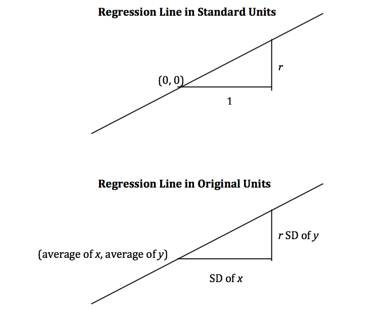
The slope and intercept of the regression line in original units can be derived from the diagram above.

$$\mathbf{\mbox{slope of the regression line}} = r \cdot
\frac{\mbox{SD of }y}{\mbox{SD of }x}$$

$$\mathbf{\mbox{intercept of the regression line}} = \mbox{average of }y - \mbox{slope} \cdot \mbox{average of }x$$

The three functions below compute the correlation, slope, and intercept. All of them take three arguments: the name of the table, the label of the column containing $x$, and the label of the column containing $y$.

Python

# Define function standard_units returning standard units
def standard_units(df):
    # Convert any array of numbers to standard units
    return (df - np.mean(df))/np.std(df)

# Define function correlation returning correlation coefficient r
def correlation(df, label_x, label_y):
    return np.mean(standard_units(df[label_x])*standard_units(df[label_y]))

# Define function slope returning slope
def slope(df, label_x, label_y):
    r = correlation(df, label_x, label_y)
    return r*np.std(df[label_y])/np.std(df[label_x])

# Define function intercet returning intercept
def intercept(df, label_x, label_y):
    return np.mean(df[label_y]) - slope(df, label_x, label_y)*np.mean(df[label_x])

---

The Regression Line in the Units of the Data

The correlation between midparent height and child’s height is 0.32:

Python

family_r = correlation(heights, 'MidParent', 'Child')
family_r
# 0.32094989606395924

We can also find the equation of the regression line for predicting the child’s height based on midparent height.

Python

family_slope = slope(heights, 'MidParent', 'Child')
family_intercept = intercept(heights, 'MidParent', 'Child')
family_slope, family_intercept
# (0.637360896969479, 22.63624054958975)

The equation of the regression line is

$$\mbox{estimate of child’s height} = 0.64 \cdot \mbox{midparent height} + 22.64$$

This is also known as the regression equation. The principal use of the regression equation is to predict $y$ based on $x$.

For example, for a midparent height of 70.48 inches, the regression equation predicts the child’s height to be 67.56 inches.

Python

family_slope * 70.48 + family_intercept
# 67.55743656799862

Our original prediction, created by taking the average height of all children who had midparent heights close to 70.48, came out to be pretty close: 67.63 inches compared to the regression line’s prediction of 67.55 inches.

Python

heights_with_predictions[heights_with_predictions.MidParent == 70.48]

	MidParent	Child	Prediction
33	70.48	74.0	67.634239
34	70.48	70.0	67.634239
35	70.48	68.0	67.634239
36	70.48	67.0	67.634239
37	70.48	67.0	67.634239
38	70.48	66.0	67.634239
39	70.48	63.5	67.634239
40	70.48	63.0	67.634239

Here are all of the rows of the table, along with our original predictions and the new regression predictions of the children’s heights.

Python

# Add Regression Prediction to DataFrame heights_with_predictions
heights_with_predictions['Regression Prediction'] = family_slope * heights.MidParent + family_intercept

heights_with_predictions

	MidParent	Child	Prediction	Regression Prediction
0	75.43	73.2	70.100000	70.712373
1	75.43	69.2	70.100000	70.712373
2	75.43	69.0	70.100000	70.712373
3	75.43	69.0	70.100000	70.712373
4	73.66	73.5	70.415789	69.584244
...	...	...	...	...
929	66.64	64.0	65.156579	65.109971
930	66.64	62.0	65.156579	65.109971
931	66.64	61.0	65.156579	65.109971
932	65.27	66.5	64.229630	64.236786
933	65.27	57.0	64.229630	64.236786

Python

# Regression Prediction and Mean Prediction
fig = go.Figure()

# Add trace MidParent & Child
fig.add_trace(go.Scatter(
    mode='markers', 
    x=heights_with_predictions['MidParent'], 
    y=heights_with_predictions['Child'], 
    name='Child', 
    marker_color='rgba(55, 73 ,99, .8)' # rgb + opacity
))
# Add trace MidParent & Prediction
fig.add_trace(go.Scatter(
    mode='markers', 
    x=heights_with_predictions['MidParent'], 
    y=heights_with_predictions['Prediction'], 
    name='Prediction', 
    marker_color='rgba(248, 202, 84, .8)' # rgb + opacity
))
# Add trace MidParent & Regression Prediction
fig.add_trace(go.Scatter(
    mode='markers', 
    x=heights_with_predictions['MidParent'], 
    y=heights_with_predictions['Regression Prediction'], 
    name='Regression Prediction', 
    marker_color='rgba(60, 160 ,207, .8)' # rgb + opacity
))
# Set layout
fig.update_layout(title="Regression Prediction and Mean Prediction", 
                  xaxis_title='MidParent', 
                  yaxis_title='', 
                  width=800,
                  height=800
)

fig.show()
# fig.write_image('fig.svg')
# ![](https://raw.githubusercontent.com/ZacksAmber/PicGo/master/img/20210425013952.svg)

The grey dots show the regression predictions, all on the regression line. Notice how the line is very close to the gold graph of averages. For these data, the regression line does a good job of approximating the centers of the vertical strips.

---

Fitted Values

The predictions all lie on the line and are known as the “fitted values”. The function fit takes the name of the table and the labels of $x$ and $y$, and returns an array of fitted values, one fitted value for each point in the scatter plot.

Python

# Define function fit returning a array of fitted values
def fit(df, x, y):
    """Return the height of the regression line at each x value."""
    a = slope(df, x, y)
    b = intercept(df, x, y)
    return a * df[x] + b

Python

# Add column Fitted to heights
heights['Fitted'] = fit(heights, 'MidParent', 'Child')

heights

	MidParent	Child	Fitted
0	75.43	73.2	70.712373
1	75.43	69.2	70.712373
2	75.43	69.0	70.712373
3	75.43	69.0	70.712373
4	73.66	73.5	69.584244
...	...	...	...
929	66.64	64.0	65.109971
930	66.64	62.0	65.109971
931	66.64	61.0	65.109971
932	65.27	66.5	64.236786
933	65.27	57.0	64.236786

Python

# Regression Prediction
fig = go.Figure()

# Add trace MidParent & Child
fig.add_trace(go.Scatter(
    mode='markers', 
    x=heights['MidParent'], 
    y=heights['Child'], 
    name='Child', 
    marker_color='rgba(55, 73 ,99, .8)' # rgb + opacity
))
# Add trace MidParent & Fitted
fig.add_trace(go.Scatter(
    mode='markers', 
    x=heights['MidParent'], 
    y=heights['Fitted'], 
    name='Fitted', 
    marker_color='rgba(60, 160 ,207, .8)' # rgb + opacity
))
# Set layout
fig.update_layout(title='Regression Prediction of Child vs. MidParent', 
                  xaxis_title='MidParent', 
                  yaxis_title='Child', 
                  width=800,
                  height=800
)

fig.show()
# fig.write_image('fig.svg')
# ![](https://raw.githubusercontent.com/ZacksAmber/PicGo/master/img/20210425020002.svg)

Another way to draw the line is to use the option mode='lines with the plotly.graph_objects method Scatter.

Python

# Regression Prediction
fig = go.Figure()

# Add trace MidParent & Child
fig.add_trace(go.Scatter(
    mode='markers', 
    x=heights['MidParent'], 
    y=heights['Child'], 
    name='Child', 
    marker_color='rgba(55, 73 ,99, .8)' # rgb + opacity
))
# Add trace MidParent & Fitted
fig.add_trace(go.Scatter(
    mode='lines', 
    x=heights['MidParent'], 
    y=heights['Fitted'], 
    name='Fitted', 
    marker_color='rgba(60, 160 ,207, .8)' # rgb + opacity
))
# Set layout
fig.update_layout(title='Regression Prediction of Child vs. MidParent', 
                  xaxis_title='MidParent', 
                  yaxis_title='Child', 
                  width=800,
                  height=800
)

fig.show()
# fig.write_image('fig.svg')
# ![](https://raw.githubusercontent.com/ZacksAmber/PicGo/master/img/20210425015900.svg)

---

Units of Measurement of the Slope

The slope is a ratio, and it worth taking a moment to study the units in which it is measured. Our example comes from the familiar dataset about mothers who gave birth in a hospital system. The scatter plot of pregnancy weights versus heights looks like a football that has been used in one game too many, but it’s close enough to a football that we can justify putting our fitted line through it. In later sections we will see how to make such justifications more formal.

Python

# Import dataset baby.csv
baby = pd.read_csv('https://github.com/ZacksAmber/Code/raw/master/Data%20Science/Data8/Data%20Sets/baby.csv')
# Add column Fitted to DataFrame baby
baby['Fitted'] = fit(baby, 'Maternal Height', 'Maternal Pregnancy Weight')

Python

# Regression Prediction
fig = go.Figure()

# Add trace MidParent & Child
fig.add_trace(go.Scatter(
    mode='markers', 
    x=baby['Maternal Height'], 
    y=baby['Maternal Pregnancy Weight'], 
    name='Maternal Pregnancy Weight', 
    marker_color='rgba(55, 73 ,99, .8)' # rgb + opacity
))
# Add trace MidParent & Fitted
fig.add_trace(go.Scatter(
    mode='lines', 
    x=baby['Maternal Height'],
    y=baby['Fitted'],
    name='Fitted', 
    marker_color='rgba(60, 160 ,207, .8)' # rgb + opacity
))
# Set layout
fig.update_layout(title='Regression Prediction of Maternal Pregnancy Weight vs. Maternal Height', 
                  xaxis_title='Maternal Height', 
                  yaxis_title='', 
                  width=800,
                  height=800
)

fig.show()
# fig.write_image('fig.svg')
# ![](https://raw.githubusercontent.com/ZacksAmber/PicGo/master/img/20210425020228.svg)

Python

slope(baby, 'Maternal Height', 'Maternal Pregnancy Weight')
# 3.572846259275056

The slope of the regression line is 3.57 pounds per inch. This means that for two women who are 1 inch apart in height, our prediction of pregnancy weight will differ by 3.57 pounds. For a woman who is 2 inches taller than another, our prediction of pregnancy weight will be

$$2 \times 3.57 = 7.14$$

pounds more than our prediction for the shorter woman.

Notice that the successive vertical strips in the scatter plot are one inch apart, because the heights have been rounded to the nearest inch. Another way to think about the slope is to take any two consecutive strips (which are necessarily 1 inch apart), corresponding to two groups of women who are separated by 1 inch in height. The slope of 3.57 pounds per inch means that the average pregnancy weight of the taller group is about 3.57 pounds more than that of the shorter group.

---

Example

Suppose that our goal is to use regression to estimate the height of a basset hound based on its weight, using a sample that looks consistent with the regression model. Suppose the observed correlation $r$ is 0.5, and that the summary statistics for the two variables are as in the table below:

	average	SD
height	14 inches	2 inches
weight	50 pounds	5 pounds

To calculate the equation of the regression line, we need the slope and the intercept.

$$\mbox{slope} = \frac{r \cdot \mbox{SD of }y}{\mbox{SD of }x} = \frac{0.5 \cdot 2 \mbox{ inches}}{5 \mbox{ pounds}} = 0.2 \mbox{inches per pound}$$

$$\mbox{intercept} = \mbox{average of }y - \mbox{slope}\cdot \mbox{average of } x = 14 \mbox{ inches} - 0.2 \mbox{ inches per pound} \cdot 50 \mbox{ pounds} = 4 \mbox{ inches}$$

The equation of the regression line allows us to calculate the estimated height, in inches, based on a given weight in pounds:

$$\mbox{estimated height} = 0.2 \cdot \mbox{given weight} + 4$$

The slope of the line is measures the increase in the estimated height per unit increase in weight. The slope is positive, and it is important to note that this does not mean that we think basset hounds get taller if they put on weight. The slope reflects the difference in the average heights of two groups of dogs that are 1 pound apart in weight. Specifically, consider a group of dogs whose weight is $w$ pounds, and the group whose weight is $w+1$ pounds. The second group is estimated to be 0.2 inches taller, on average. This is true for all values of $w$ in the sample.

In general, the slope of the regression line can be interpreted as the average increase in $y$ per unit increase in $x$. Note that if the slope is negative, then for every unit increase in $x$, the average of $y$ decreases.

---

Endnote

Even though we won’t establish the mathematical basis for the regression equation, we can see that it gives pretty good predictions when the scatter plot is football shaped. It is a surprising mathematical fact that no matter what the shape of the scatter plot, the same equation gives the “best” among all straight lines. That’s the topic of the next section.

---

The Method of Least Squares

https://inferentialthinking.com/chapters/15/3/Method_of_Least_Squares.html

We have developed the equation of the regression line that runs through a football shaped scatter plot. But not all scatter plots are football shaped, not even linear ones. Does every scatter plot have a “best” line that goes through it? If so, can we still use the formulas for the slope and intercept developed in the previous section, or do we need new ones?

To address these questions, we need a reasonable definition of “best”. Recall that the purpose of the line is to predict or estimate values of $y$, given values of $x$. Estimates typically aren’t perfect. Each one is off the true value by an error. A reasonable criterion for a line to be the “best” is for it to have the smallest possible overall error among all straight lines.

In this section we will make this criterion precise and see if we can identify the best straight line under the criterion.

Our first example is a dataset that has one row for every chapter of the novel “Little Women.” The goal is to estimate the number of characters (that is, letters, spaces punctuation marks, and so on) based on the number of periods. Recall that we attempted to do this in the very first lecture of this course.

Python

# Import dataset little_women.csv
little_women = pd.read_csv('https://github.com/ZacksAmber/Code/raw/master/Data%20Science/Data8/Data%20Sets/little_women.csv')
little_women.head(3)

	Characters	Periods
0	21759	189
1	22148	188
2	20558	231

Python

# Reverse the columns name
cols = list(reversed(list(little_women.columns)))
# Reorder the columns in cols sequence
little_women = little_women.loc[:, cols]

little_women.head(3)

	Periods	Characters
0	189	21759
1	188	22148
2	231	20558

Python

# Scatter of Characters vs. Periods
fig = go.Figure()

# Add trace Periods & Characters
fig.add_trace(go.Scatter(
    mode='markers', 
    x=little_women['Periods'], 
    y=little_women['Characters'], 
    name='Characters', 
    marker_color='rgba(55, 73 ,99, .8)' # rgb + opacity
))
# Set layout
fig.update_layout(title='Scatter of Characters vs. Periods', 
                  # xaxis_title='Maternal Height', 
                  # yaxis_title='', 
                  width=800,
                  height=800
)

fig.show()
# fig.write_image('fig.svg')
# ![](https://raw.githubusercontent.com/ZacksAmber/PicGo/master/img/20210425225337.svg)

To explore the data, we will need to use the functions correlation, slope, intercept, and fit defined in the previous section.

Python

correlation(little_women, 'Periods', 'Characters')
# 0.9229576895854816

The scatter plot is remarkably close to linear, and the correlation is more than 0.92.

---

Error in Estimation

The graph below shows the scatter plot and line that we developed in the previous section. We don’t yet know if that’s the best among all lines. We first have to say precisely what “best” means.

Python

# Copy little_women to lw_with_predictions
lw_with_predictions = little_women.copy()
# Add fitted value Linear Prediction to lw_with_predictions
lw_with_predictions['Linear Prediction'] = fit(little_women, 'Periods', 'Characters')

lw_with_predictions

	Periods	Characters	Linear Prediction
0	189	21759	21183.596794
1	188	22148	21096.618953
2	231	20558	24836.666127
3	195	25526	21705.463842
4	255	23395	26924.134317
...	...	...	...
42	305	33202	31273.026380
43	95	10289	13007.679716
44	96	12558	13094.657557
45	234	27094	25097.599651
46	392	40935	38840.098570

Python

# Linear Regression Prediction
fig = go.Figure()

# Add trace Periods & Characters
fig.add_trace(go.Scatter(
    mode='markers', 
    x=lw_with_predictions['Periods'], 
    y=lw_with_predictions['Characters'], 
    name='Characters', 
    marker_color='rgba(55, 73 ,99, .8)' # rgb + opacity
))
# Add trace Periods & Linear Prediction
fig.add_trace(go.Scatter(
    mode='markers', 
    x=lw_with_predictions['Periods'], 
    y=lw_with_predictions['Linear Prediction'], 
    name='Linear Prediction', 
    marker_color='rgba(248, 202, 84, .8)' # rgb + opacity
))
# Set layout
fig.update_layout(title='Linear Regression Prediction of Characters vs. Periods', 
                  xaxis_title='Periods', 
                  yaxis_title='', # Remove yaxis titile
                  width=800,
                  height=800
)

fig.show()
# fig.write_image('fig.svg')
# ![](https://raw.githubusercontent.com/ZacksAmber/PicGo/master/img/20210426000555.svg)

Corresponding to each point on the scatter plot, there is an error of prediction calculated as the actual value minus the predicted value. It is the vertical distance between the point and the line, with a negative sign if the point is below the line.

Python

# y
actual = lw_with_predictions['Characters']
# Predicted y
predicted = lw_with_predictions['Linear Prediction']
# Errors = y - Predicted y
errors = actual - predicted

Python

# Add errors to lw_with_predictions
lw_with_predictions['Error'] = errors

lw_with_predictions

	Periods	Characters	Linear Prediction	Error
0	189	21759	21183.596794	575.403206
1	188	22148	21096.618953	1051.381047
2	231	20558	24836.666127	-4278.666127
3	195	25526	21705.463842	3820.536158
4	255	23395	26924.134317	-3529.134317
...	...	...	...	...
42	305	33202	31273.026380	1928.973620
43	95	10289	13007.679716	-2718.679716
44	96	12558	13094.657557	-536.657557
45	234	27094	25097.599651	1996.400349
46	392	40935	38840.098570	2094.901430

We can use slope and intercept to calculate the slope and intercept of the fitted line. The graph below shows the line (in light blue). The errors corresponding to four of the points are shown in red. There is nothing special about those four points. They were just chosen for clarity of the display. The function lw_errors takes a slope and an intercept (in that order) as its arguments and draws the figure.

Python

# Call function slope and intercept
lw_reg_slope = slope(little_women, 'Periods', 'Characters')
lw_reg_intercept = intercept(little_women, 'Periods', 'Characters')

Python

sample = [[131, 14431], [231, 20558], [392, 40935], [157, 23524]]
def lw_errors(slope, intercept, rmse=None):
    # Linear Regression Prediction with 4 sample errors
    fig = go.Figure()

    # Add trace Periods & Characters
    fig.add_trace(go.Scatter(
        mode='markers', 
        x=lw_with_predictions['Periods'], 
        y=lw_with_predictions['Characters'], 
        name='Characters', 
        marker_color='rgba(55, 73 ,99, .8)' # rgb + opacity
    ))
    # Add trace Periods & Linear Prediction
    fig.add_trace(go.Scatter(
        mode='lines', 
        x=lw_with_predictions['Periods'], 
        y=lw_with_predictions['Periods'] * slope + intercept, 
        name='Linear Prediction', 
        marker_color='rgba(60, 160 ,207, .8)' # rgb + opacity
    ))
    # Set layout
    title='Linear Regression Prediction of Characters vs. Periods with 4 sample errors'
    title+=f'<br>Slope of Regression Line: {np.round(slope)} characters per period' # Add slope to title. <br> next line in HTML
    title+=f'<br>Intercept of Regression Line: {np.round(intercept)} characters' # Add error to title. <br> next line in HTML
    if rmse != None:
        title+=f'<br>Root mean squared error: {rmse}' # Add rmse to title. <br> next line in HTML
    fig.update_layout(title=title, 
                      xaxis_title='Periods', 
                      yaxis_title='Characters',
                      width=800,
                      height=800
    )
    # Calculate 4 sample predicted y
    # Add 4 sample errors based on linear regression
    for x, y in sample:
        y1 = x * slope + intercept
        # Add sample errors
        fig.add_shape(type='line', 
                      x0=x, y0=y, 
                      x1=x, y1=y1, 
                      line_color='red')

    fig.show()
    fig.write_image('fig.svg')

Python

lw_errors(lw_reg_slope, lw_reg_intercept)
# ![](https://raw.githubusercontent.com/ZacksAmber/PicGo/master/img/20210426010322.svg)

Had we used a different line to create our estimates, the errors would have been different. The graph below shows how big the errors would be if we were to use another line for estimation. The second graph shows large errors obtained by using a line that is downright silly.

Python

lw_errors(50, 10000)
# ![](https://raw.githubusercontent.com/ZacksAmber/PicGo/master/img/20210426010443.svg)

Python

lw_errors(-100, 50000)
# ![](https://raw.githubusercontent.com/ZacksAmber/PicGo/master/img/20210426010554.svg)

---

Root Mean Squared Error

What we need now is one overall measure of the rough size of the errors. You will recognize the approach to creating this – it’s exactly the way we developed the SD.

If you use any arbitrary line to calculate your estimates, then some of your errors are likely to be positive and others negative. To avoid cancellation when measuring the rough size of the errors, we will take the mean of the squared errors rather than the mean of the errors themselves.

The mean squared error of estimation is a measure of roughly how big the squared errors are, but as we have noted earlier, its units are hard to interpret. Taking the square root yields the root mean square error (rmse), which is in the same units as the variable being predicted and therefore much easier to understand.

---

Minimizing the Root Mean Squared Error

Our observations so far can be summarized as follows.

• To get estimates of $y$ based on $x$, you can use any line you want.
• Every line has a root mean squared error of estimation.
• “Better” lines have smaller errors.

Is there a “best” line? That is, is there a line that minimizes the root mean squared error among all lines?

To answer this question, we will start by defining a function lw_rmse to compute the root mean squared error of any line through the Little Women scatter diagram. The function takes the slope and the intercept (in that order) as its arguments.

Python

# Define function lw_rmse returning root mean square error
def lw_rmse(slope, intercept):
    x = little_women['Periods']
    y = little_women['Characters']
    fitted = slope * x + intercept
    mse = np.mean((y - fitted) ** 2)
    rmse = mse ** 0.5
    lw_errors(slope, intercept, np.round(rmse, 2)) # Also pass rmse to function lw_errors

Python

lw_rmse(50, 10000)
# ![](https://raw.githubusercontent.com/ZacksAmber/PicGo/master/img/20210426015111.svg)

Python

lw_rmse(-100, 50000)
# ![](https://raw.githubusercontent.com/ZacksAmber/PicGo/master/img/20210426015231.svg)

Bad lines have big values of rmse, as expected. But the rmse is much smaller if we choose a slope and intercept close to those of the regression line.

Python

lw_rmse(90, 4000)
# ![](https://raw.githubusercontent.com/ZacksAmber/PicGo/master/img/20210426015333.svg)

Here is the root mean squared error corresponding to the regression line. By a remarkable fact of mathematics, no other line can beat this one.

• The regression line is the unique straight line that minimizes the mean squared error of estimation among all straight lines.

Python

lw_rmse(lw_reg_slope, lw_reg_intercept)
# ![](https://raw.githubusercontent.com/ZacksAmber/PicGo/master/img/20210426015441.svg)

The proof of this statement requires abstract mathematics that is beyond the scope of this course. On the other hand, we do have a powerful tool – Python – that performs large numerical computations with ease. So we can use Python to confirm that the regression line minimizes the mean squared error.

---

Numerical Optimization

First note that a line that minimizes the root mean squared error is also a line that minimizes the squared error. The square root makes no difference to the minimization. So we will save ourselves a step of computation and just minimize the mean squared error (mse).

We are trying to predict the number of characters ($y$) based on the number of periods ($x$) in chapters of Little Women. If we use the line

$$\mbox{prediction} = ax + b$$

it will have an mse that depends on the slope $a$ and the intercept $b$. The function lw_mse takes the slope and intercept as its arguments and returns the corresponding mse.

Let’s check that lw_mse gets the right answer for the root mean squared error of the regression line. Remember that lw_mse returns the mean squared error, so we have to take the square root to get the rmse.

Python

def lw_mse(any_slope, any_intercept):
    x = little_women['Periods']
    y = little_women['Characters']
    fitted = any_slope*x + any_intercept
    return np.mean((y - fitted) ** 2)

Python

lw_mse(lw_reg_slope, lw_reg_intercept)**0.5
# 2701.690785311856

That’s the same as the value we got by using lw_rmse earlier:

Python

lw_rmse(lw_reg_slope, lw_reg_intercept)
# ![](https://raw.githubusercontent.com/ZacksAmber/PicGo/master/img/20210426021905.svg)

You can confirm that lw_mse returns the correct value for other slopes and intercepts too. For example, here is the rmse of the extremely bad line that we tried earlier.

Python

lw_mse(-100, 50000)**0.5
# 16710.11983735375

And here is the rmse for a line that is close to the regression line.

Python

lw_mse(90, 4000)**0.5
# 2715.5391063834586

If we experiment with different values, we can find a low-error slope and intercept through trial and error, but that would take a while. Fortunately, there is a Python function that does all the trial and error for us.

The scipy.optimize.minimize function can be used to find the arguments of a function for which the function returns its minimum value. Python uses a similar trial-and-error approach, following the changes that lead to incrementally lower output values.

The argument of scipy.optimize.minimize is a function that itself takes numerical arguments and returns a numerical value. For example, the function lw_mse takes a numerical slope and intercept as its arguments and returns the corresponding mse.

The call minimize(lw_mse) returns an array consisting of the slope and the intercept that minimize the mse. These minimizing values are excellent approximations arrived at by intelligent trial-and-error, not exact values based on formulas.

scipy.optimize.minimize

Let’s update function lw_mse. Combine parameter any_slope and any_intercept to Optimization

Python

# Combine parameter any_slope and any_intercept to Optimization
def lw_mse(Optimization):
    x = little_women['Periods']
    y = little_women['Characters']
    fitted = Optimization[0]*x + Optimization[1]
    return np.mean((y - fitted) ** 2)

Python

from scipy.optimize import minimize
# Initialize Optimization
x0 = np.array([1, 1])

# Minimize lw_mse
res = minimize(lw_mse, x0, method='Nelder-Mead')

print(res)
'''
 final_simplex: (array([[  86.97784154, 4744.78478432],
       [  86.97784166, 4744.78468544],
       [  86.9778411 , 4744.78483106]]), array([7299133.09943899, 7299133.099439  , 7299133.099439  ]))
           fun: 7299133.099438994
       message: 'Optimization terminated successfully.'
          nfev: 219
           nit: 114
        status: 0
       success: True
             x: array([  86.97784154, 4744.78478432])

Python

res.x
# array([  86.97784154, 4744.78478432])

Python

print("slope from formula:        ", lw_reg_slope)
print("slope from minimize:       ", res.x[0])
print("intercept from formula:    ", lw_reg_intercept)
print("intercept from minimize:   ", res.x[1])
'''
slope from formula:         86.97784125829821
slope from minimize:        86.97784153846081
intercept from formula:     4744.784796574928
intercept from minimize:    4744.784784318655
'''

---

The Least Squares Line

Therefore, we have found not only that the regression line minimizes mean squared error, but also that minimizing mean squared error gives us the regression line. The regression line is the only line that minimizes mean squared error.

That is why the regression line is sometimes called the “least squares line.”

These values are the same as the values we calculated earlier by using the slope and intercept functions. We see small deviations due to the inexact nature of minimize, but the values are essentially the same.

---

Least Squares Regression

In an earlier section, we developed formulas for the slope and intercept of the regression line through a football shaped scatter diagram. It turns out that the slope and intercept of the least squares line have the same formulas as those we developed, regardless of the shape of the scatter plot.

We saw this in the example about Little Women, but let’s confirm it in an example where the scatter plot clearly isn’t football shaped. For the data, we are once again indebted to the rich data archive of Prof. Larry Winner of the University of Florida. A 2013 study in the International Journal of Exercise Science studied collegiate shot put athletes and examined the relation between strength and shot put distance. The population consists of 28 female collegiate athletes. Strength was measured by the the biggest amount (in kilograms) that the athlete lifted in the “1RM power clean” in the pre-season. The distance (in meters) was the athlete’s personal best.

Pyhon

# Import dataset shotput.csv
shotput = pd.read_csv('https://github.com/ZacksAmber/Code/raw/master/Data%20Science/Data8/Data%20Sets/shotput.csv')
shotput

	Weight Lifted	Shot Put Distance
0	37.5	6.4
1	51.5	10.2
2	61.3	12.4
3	61.3	13.0
4	63.6	13.2
...	...	...
23	123.6	16.8
24	125.8	17.0
25	119.1	18.2
26	118.9	19.2
27	141.1	18.6

Python

# Scatter of Shot Put Distance vs. Weight Lifted
fig = go.Figure()

# Add trace Shot Put Distance &. Weight Lifted
fig.add_trace(go.Scatter(
    mode='markers', 
    x=shotput['Weight Lifted'], 
    y=shotput['Shot Put Distance'], 
    name='Shot Put Distance', 
    marker_color='rgba(55, 73 ,99, .8)' # rgb + opacity
))
# Set layout
fig.update_layout(title='Scatter of Shot Put Distance vs. Weight Lifted', 
                  xaxis_title='Weight Lifted', 
                  yaxis_title='Shot Put Distance', 
                  height=800, 
                  width=800
)

fig.show()
# fig.write_image('fig.svg')
# ![](https://raw.githubusercontent.com/ZacksAmber/PicGo/master/img/20210426172457.svg)

That’s not a football shaped scatter plot. In fact, it seems to have a slight non-linear component. But if we insist on using a straight line to make our predictions, there is still one best straight line among all straight lines.

Our formulas for the slope and intercept of the regression line, derived for football shaped scatter plots, give the following values.

Python

slope(shotput, 'Weight Lifted', 'Shot Put Distance')
# 0.09834382159781997

Python

intercept(shotput, 'Weight Lifted', 'Shot Put Distance')
# 5.959629098373952

Does it still make sense to use these formulas even though the scatter plot isn’t football shaped? We can answer this by finding the slope and intercept of the line that minimizes the mse.

We will define the function shotput_linear_mse to take an arbirtary slope and intercept as arguments and return the corresponding mse. Then minimize applied to shotput_linear_mse will return the best slope and intercept.

Python

# Combine parameter any_slope and any_intercept to Optimization
def shotput_linear_mse(Optimization: list):
    x = shotput['Weight Lifted']
    y = shotput['Shot Put Distance']
    fitted = Optimization[0]*x + Optimization[1]
    return np.mean((y - fitted) ** 2)

Python

from scipy.optimize import minimize
# Initialize Optimization
x0 = np.array([1, 1])

# Minimize shotput_linear_mse
res = minimize(shotput_linear_mse, x0, method='Nelder-Mead')

print(res)
'''
 final_simplex: (array([[0.09834369, 5.95964193],
       [0.09834434, 5.95957953],
       [0.09834393, 5.95960397]]), array([1.48704485, 1.48704485, 1.48704485]))
           fun: 1.4870448508028293
       message: 'Optimization terminated successfully.'
          nfev: 138
           nit: 75
        status: 0
       success: True
             x: array([0.09834369, 5.95964193])
'''

Python

res.x
# array([0.09834369, 5.95964193])

These values are the same as those we got by using our formulas. To summarize:

No matter what the shape of the scatter plot, there is a unique line that minimizes the mean squared error of estimation. It is called the regression line, and its slope and intercept are given by

$$\mathbf{\mbox{slope of the regression line}} = r \cdot\frac{\mbox{SD of }y}{\mbox{SD of }x}$$

$$\mathbf{\mbox{intercept of the regression line}} = \mbox{average of }y - \mbox{slope} \cdot \mbox{average of }x$$

Python

# Calculuate the fitted value
fitted = fit(shotput, 'Weight Lifted', 'Shot Put Distance')
shotput['Best Straight Line'] = fitted

shotput

	Weight Lifted	Shot Put Distance	Best Straight Line
0	37.5	6.4	9.647522
1	51.5	10.2	11.024336
2	61.3	12.4	11.988105
3	61.3	13.0	11.988105
4	63.6	13.2	12.214296
...	...	...	...
23	123.6	16.8	18.114925
24	125.8	17.0	18.331282
25	119.1	18.2	17.672378
26	118.9	19.2	17.652709
27	141.1	18.6	19.835942

Python

# Linear Regression Prediction
fig = go.Figure()

# Add trace Shot Put Distance &. Weight Lifted
fig.add_trace(go.Scatter(
    mode='markers', 
    x=shotput['Weight Lifted'], 
    y=shotput['Shot Put Distance'], 
    name='Shot Put Distance', 
    marker_color='rgba(55, 73 ,99, .8)' # rgb + opacity
))
# Add trace Shot Put Distance &. Linear Prediction
fig.add_trace(go.Scatter(
    mode='markers', 
    x=shotput['Weight Lifted'], 
    y=shotput['Best Straight Line'], 
    name='Linear Prediction', 
    marker_color='rgba(248, 202, 84, .8)' # rgb + opacity
))
# Set layout
fig.update_layout(title='Linear Regression Prediction of Shot Put Distance vs. Weight Lifted', 
                  xaxis_title='Weight Lifted', 
                  #yaxis_title='Shot Put Distance'
                  height=800, 
                  width=800
)

fig.show()
# fig.write_image('fig.svg')
# ![](https://raw.githubusercontent.com/ZacksAmber/PicGo/master/img/20210430113143.svg)

---

Nonlinear Regression

The graph above reinforces our earlier observation that the scatter plot is a bit curved. So it is better to fit a curve than a straight line. The study postulated a quadratic relation between the weight lifted and the shot put distance. So let’s use quadratic functions as our predictors and see if we can find the best one.

We have to find the best quadratic function among all quadratic functions, instead of the best straight line among all straight lines. The method of least squares allows us to do this.

The mathematics of this minimization is complicated and not easy to see just by examining the scatter plot. But numerical minimization is just as easy as it was with linear predictors! We can get the best quadratic predictor by once again using minimize. Let’s see how this works.

Recall that a quadratic function has the form

$$f(x) = ax^2 + bx + c$$

for constants $a$, $b$, and $c$.

To find the best quadratic function to predict distance based on weight lifted, using the criterion of least squares, we will first write a function that takes the three constants as its arguments, calculates the fitted values by using the quadratic function above, and then returns the mean squared error.

The function is called shotput_quadratic_mse. Notice that the definition is analogous to that of lw_mse, except that the fitted values are based on a quadratic function instead of linear.

Python

def shotput_quadratic_mse(Optimization):
    a = Optimization[0]
    b = Optimization[1]
    c = Optimization[2]
    x = shotput['Weight Lifted']
    y = shotput['Shot Put Distance']
    fitted = a*(x**2) + b*x + c
    return np.mean((y - fitted) ** 2)

Python

from scipy.optimize import minimize
# Initialize Optimization
x0 = np.array([1, 1, 1])

# Minimize shotput_linear_mse
res = minimize(shotput_quadratic_mse, x0, method='L-BFGS-B')

res.x
# array([-1.04118928e-03,  2.82913118e-01, -1.54027074e+00])

Our prediction of the shot put distance for an athlete who lifts $x$ kilograms is about

$$-0.00104x^2 + 0.2827x - 1.5318$$

meters. For example, if the athlete can lift 100 kilograms, the predicted distance is 16.33 meters. On the scatter plot, that’s near the center of a vertical strip around 100 kilograms.

Python

(-0.00104)*(100**2) + 0.2827*100 - 1.5318
# 16.3382

Here are the predictions for all the values of Weight Lifted. You can see that they go through the center of the scatter plot, to a rough approximation.

Python

# Calculate fitted value by nonlieaner regression
x = shotput['Weight Lifted']
a = res.x[0]
b = res.x[1]
c = res.x[2]
shotput_fit = a*(x**2) + b*x + c

Python

# Add shotput_fit to shotput
shotput['Best Quadratic Curve'] = shotput_fit

shotput

	Weight Lifted	Shot Put Distance	Best Straight Line	Best Quadratic Curve
0	37.5	6.4	9.647522	7.604799
1	51.5	10.2	11.024336	10.268261
2	61.3	12.4	11.988105	11.889837
3	61.3	13.0	11.988105	11.889837
4	63.6	13.2	12.214296	12.241435
...	...	...	...	...
23	123.6	16.8	18.114925	17.521584
24	125.8	17.0	18.331282	17.572713
25	119.1	18.2	17.672378	17.385610
26	118.9	19.2	17.652709	17.378588
27	141.1	18.6	19.835942	17.649514

Python

# Nonlinear Regression Prediction
fig = go.Figure()

# Add trace Shot Put Distance &. Weight Lifted
fig.add_trace(go.Scatter(
    mode='markers', 
    x=shotput['Weight Lifted'], 
    y=shotput['Shot Put Distance'], 
    name='Shot Put Distance', 
    marker_color='rgba(55, 73 ,99, .8)' # rgb + opacity
))
# Add trace Shot Put Distance &. Nonlinear Prediction
fig.add_trace(go.Scatter(
    mode='markers', 
    x=shotput['Weight Lifted'], 
    y=shotput['Best Quadratic Curve'], 
    name='Nonlinear Prediction', 
    marker_color='rgba(248, 202, 84, .8)' # rgb + opacity
))
# Set layout
fig.update_layout(title='Nonlinear Regression Prediction of Shot Put Distance vs. Weight Lifted', 
                  xaxis_title='Weight Lifted', 
                  #yaxis_title='Shot Put Distance'
                  height=800, 
                  width=800
)

fig.show()
# fig.write_image('fig.svg')
# ![](https://raw.githubusercontent.com/ZacksAmber/PicGo/master/img/20210426175054.svg)

Note: We fit a quadratic here because it was suggested in the original study. But it is worth noting that at the rightmost end of the graph, the quadratic curve appears to be close to peaking, after which the curve will start going downwards. So we might not want to use this model for new athletes who can lift weights much higher than those in our data set.

---

Visual Diagnostics

Suppose a data scientist has decided to use linear regression to estimate values of one variable (called the response variable) based on another variable (called the predictor). To see how well this method of estimation performs, the data scientist must measure how far off the estimates are from the actual values. These differences are called residuals.

$$\mbox{residual} = \mbox{observed value} - \mbox{regression estimate}$$

A residual is what’s left over – the residue – after estimation.

Residuals are the vertical distances of the points from the regression line. There is one residual for each point in the scatter plot. The residual is the difference between the observed value of $y$ and the fitted value of $y$, so for the point $(x, y)$,

$$\mbox{residual} = y - \mbox{fitted value of }y = y - \mbox{height of regression line at }x$$

The function residual calculates the residuals. The calculation assumes all the relevant functions we have already defined: standard_units, correlation, slope, intercept, and fit.

Python

# Define function resudual returning residuals
def residual(df, x, y):
    return df[y] - fit(df, x, y)

Continuing our example of estimating the heights of adult children (the response) based on the midparent height (the predictor), let us calculate the fitted values and the residuals.

Python

# Import dataset galton.csv
# Data on heights of parents and their adult children
original = pd.read_csv('https://github.com/ZacksAmber/Code/raw/master/Data%20Science/Data8/Data%20Sets/galton.csv')
heights = pd.DataFrame({
    'MidParent': original['midparentHeight'],
    'Child': original['childHeight']
})

heights

Python

# Add Fitted Value to heights
heights['Fitted Value'] = fit(heights, 'MidParent', 'Child')
# Add Residual to heights
heights['Residual'] = residual(heights, 'MidParent', 'Child')

heights

	MidParent	Child	Fitted Value	Residual
0	75.43	73.2	70.712373	2.487627
1	75.43	69.2	70.712373	-1.512373
2	75.43	69.0	70.712373	-1.712373
3	75.43	69.0	70.712373	-1.712373
4	73.66	73.5	69.584244	3.915756
...	...	...	...	...
929	66.64	64.0	65.109971	-1.109971
930	66.64	62.0	65.109971	-3.109971
931	66.64	61.0	65.109971	-4.109971
932	65.27	66.5	64.236786	2.263214
933	65.27	57.0	64.236786	-7.236786

When there are so many variables to work with, it is always helpful to start with visualization. The function scatter_fit draws the scatter plot of the data, as well as the regression line.

Python

# Define function scatter_fit returning scatter and regression
def scatter_fit(df, x, y):
    # Nonlinear Regression Prediction
    fig = go.Figure()

    # Add trace x &. y
    fig.add_trace(go.Scatter(
        mode='markers', 
        x=df[x], 
        y=df[y], 
        name=y, 
        marker_color='rgba(55, 73 ,99, .8)' # rgb + opacity
    ))
    # Calculate fitted value
    df['Fitted Value'] = fit(df, x, y)
    # Add trace x &. Prediction
    fig.add_trace(go.Scatter(
        mode='lines', 
        x=df[x], 
        y=df['Fitted Value'], 
        name='Prediction', 
        marker_color='rgba(248, 202, 84, .8)' # rgb + opacity
    ))
    # Set layout
    title = f'Prediction of {y} vs. {x}'
    fig.update_layout(title=title, 
                      xaxis_title=x, 
                      yaxis_title=y, 
                      height=800, 
                      width=800
    )

    fig.show()
    fig.write_image('fit.svg')

Python

scatter_fit(heights, 'MidParent', 'Child')
# ![](https://raw.githubusercontent.com/ZacksAmber/PicGo/master/img/20210426222335.svg)

A residual plot can be drawn by plotting the residuals against the predictor variable. The function residual_plot does just that.

Python

# Define function residual_plot returning residuals and prediction
def residual_plot(df, x, y):
    # Nonlinear Regression Prediction
    fig = go.Figure()

    # Calculate residuals
    df['Residual'] = residual(df, x, y)
    # Add trace x &. Resiudals
    fig.add_trace(go.Scatter(
        mode='markers', 
        x=df[x], 
        y=df['Residual'], 
        name='Residual', 
        marker_color='rgba(246, 46, 56, .8)' # rgb + opacity
    ))
    # Add horizontal axis
    fig.add_shape(type='line', x0=min(df[x]), y0=0, x1=max(df[x]), y1=0, line_color='rgba(0, 0, 120, .8)')
    # Set layout
    title = f'Residual Plot'
    fig.update_layout(title=title, 
                      xaxis_title=x, 
                      yaxis_title='Residuals', 
                      height=800, 
                      width=800
    )

    fig.show()
    fig.write_image('fig.svg')

Python

residual_plot(heights, 'MidParent', 'Child')
# ![](https://raw.githubusercontent.com/ZacksAmber/PicGo/master/img/20210426205203.svg)

The midparent heights are on the horizontal axis, as in the original scatter plot. But now the vertical axis shows the residuals. Notice that the plot appears to be centered around the horizontal line at the level 0 (shown in dark blue). Notice also that the plot shows no upward or downward trend. We will observe later that this lack of trend is true of all regressions.

---

Regression Diagnostics

Residual plots help us make visual assessments of the quality of a linear regression analysis. Such assessments are called diagnostics. The function regression_diagnostic_plots draws the original scatter plot as well as the residual plot for ease of comparison.

Python

# Define function regression_diagnostic_plots returning Prediction and Residual Plot
def regression_diagnostic_plots(table, x, y):
    scatter_fit(table, x, y)
    residual_plot(table, x, y)

Python

regression_diagnostic_plots(heights, 'MidParent', 'Child')
# ![](https://raw.githubusercontent.com/ZacksAmber/PicGo/master/img/20210426222417.svg)
# ![](https://raw.githubusercontent.com/ZacksAmber/PicGo/master/img/20210426222430.svg)

This residual plot indicates that linear regression was a reasonable method of estimation. Notice how the residuals are distributed fairly symmetrically above and below the horizontal line at 0, corresponding to the original scatter plot being roughly symmetrical above and below. Notice also that the vertical spread of the plot is fairly even across the most common values of the children’s heights. In other words, apart from a few outlying points, the plot isn’t narrower in some places and wider in others.

In other words, the accuracy of the regression appears to be about the same across the observed range of the predictor variable.

The residual plot of a good regression shows no pattern. The residuals look about the same, above and below the horizontal line at 0, across the range of the predictor variable.

---

Detecting Nonlinearity

Drawing the scatter plot of the data usually gives an indication of whether the relation between the two variables is non-linear. Often, however, it is easier to spot non-linearity in a residual plot than in the original scatter plot. This is usually because of the scales of the two plots: the residual plot allows us to zoom in on the errors and hence makes it easier to spot patterns.

Our data are a dataset on the age and length of dugongs, which are marine mammals related to manatees and sea cows (image from Wikimedia Commons). The data are in a table called dugong. Age is measured in years and length in meters. Because dugongs tend not to keep track of their birthdays, ages are estimated based on variables such as the condition of their teeth.

Python

# Import dataset dugongs.csv
dugong = pd.read_csv('https://github.com/ZacksAmber/Code/raw/master/Data%20Science/Data8/Data%20Sets/dugong.csv')
# Reverse the columns name
cols = list(dugong.columns)
cols.reverse()
# Reorder the columns in cols sequence
dugong.loc[:, cols]

	Age	Length
0	1.0	1.80
1	1.5	1.85
2	1.5	1.87
3	1.5	1.77
4	2.5	2.02
...	...	...
22	16.5	2.64
23	17.0	2.56
24	22.5	2.70
25	29.0	2.72
26	31.5	2.57

If we could measure the length of a dugong, what could we say about its age? Let’s examine what our data say. Here is a regression of age (the response) on length (the predictor). The correlation between the two variables is substantial, at 0.83.

Python

correlation(dugong, 'Length', 'Age')
# 0.8296474554905714

High correlation notwithstanding, the plot shows a curved pattern that is much more visible in the residual plot.

Python

regression_diagnostic_plots(dugong, 'Length', 'Age')
# ![](https://raw.githubusercontent.com/ZacksAmber/PicGo/master/img/20210426222516.svg)
# ![](https://raw.githubusercontent.com/ZacksAmber/PicGo/master/img/20210426221631.svg)

While you can spot the non-linearity in the original scatter, it is more clearly evident in the residual plot.

At the low end of the lengths, the residuals are almost all positive; then they are almost all negative; then positive again at the high end of lengths. In other words the regression estimates have a pattern of being too high, then too low, then too high. That means it would have been better to use a curve instead of a straight line to estimate the ages.

When a residual plot shows a pattern, there may be a non-linear relation between the variables.

---

Detecting Heteroscedasticity

Heteroscedasticity is a word that will surely be of interest to those who are preparing for Spelling Bees. For data scientists, its interest lies in its meaning, which is “uneven spread”.

Recall the table hybrid that contains data on hybrid cars in the U.S. Here is a regression of fuel efficiency on the rate of acceleration. The association is negative: cars that accelearate quickly tend to be less efficient.

Python

# Import dataset hybrid.csv
hybrid = pd.read_csv('https://github.com/ZacksAmber/Code/raw/master/Data%20Science/Data8/Data%20Sets/hybrid.csv')

Python

regression_diagnostic_plots(hybrid, 'acceleration', 'mpg')
# ![](https://raw.githubusercontent.com/ZacksAmber/PicGo/master/img/20210426222815.svg)
# ![](https://raw.githubusercontent.com/ZacksAmber/PicGo/master/img/20210426222825.svg)

Notice how the residual plot flares out towards the low end of the accelerations. In other words, the variability in the size of the errors is greater for low values of acceleration than for high values. Uneven variation is often more easily noticed in a residual plot than in the original scatter plot.

If the residual plot shows uneven variation about the horizontal line at 0, the regression estimates are not equally accurate across the range of the predictor variable.

---

Numerical Diagnostics

In addition to visualization, we can use numerical properties of residuals to assess the quality of regression. We will not prove these properties mathematically. Rather, we will observe them by computation and see what they tell us about the regression.

All of the facts listed below hold for all shapes of scatter plots, whether or not they are linear.

---

Residual Plots Show No Trend

For every linear regression, whether good or bad, the residual plot shows no trend. Overall, it is flat. In other words, the residuals and the predictor variable are uncorrelated.

You can see this in all the residual plots above. We can also calculate the correlation between the predictor variable and the residuals in each case.

Python

correlation(heights, 'MidParent', 'Residual')
# -2.719689807647064e-16

That doesn’t look like zero, but it is a tiny number that is 0 apart from rounding error due to computation. Here it is again, correct to 10 decimal places. The minus sign is because of the rounding that above.

Python

round(correlation(heights, 'MidParent', 'Residual'), 10)
# -0.0

Python

round(correlation(dugong, 'Length', 'Residual'), 10)
# 0.0

---

Average of Residuals

No matter what the shape of the scatter diagram, the average of the residuals is 0.

This is analogous to the fact that if you take any list of numbers and calculate the list of deviations from average, the average of the deviations is 0.

In all the residual plots above, you have seen the horizontal line at 0 going through the center of the plot. That is a visualization of this fact.

As a numerical example, here is the average of the residuals in the regression of children’s heights based on midparent heights.

Python

round(np.mean(heights['Residual']), 10)
# 0.0

The same is true of the average of the residuals in the regression of the age of dugongs on their length. The mean of the residuals is 0, apart from rounding error.

Python

round(np.mean(dugong['Residual']), 10)
# 0.0

---

SD of the Residuals

No matter what the shape of the scatter plot, the SD of the residuals is a fraction of the SD of the response variable. The fraction is $\sqrt{1-r^2}$

$$\mbox{SD of residuals} = \sqrt{1 - r^2} \cdot \mbox{SD of }y$$

We will soon see how this measures the accuracy of the regression estimate. But first, let’s confirm it by example.

In the case of children’s heights and midparent heights, the SD of the residuals is about 3.39 inches.

Python

np.std(heights['Residual'])
# 3.3880799163953426

Python

np.std(dugong['Residual'])
# 4.3113328602881555

Python

np.std(hybrid['Residual'])
# 9.43273683343029

That’s the same as $\sqrt{1-r^2}$ times the SD of response variable:

Python

r = correlation(heights, 'MidParent', 'Child')
np.sqrt(1 - r**2) * np.std(heights['Child'])
# 3.3880799163953426

The same is true for the regression of mileage on acceleration of hybrid cars. The correlation $r$ is negative (about -0.5), but $r^2$ is positive and therefore $\sqrt{1-r^2}$ is a fraction.

Python

r = correlation(hybrid, 'acceleration', 'mpg')
r
# -0.5060703843771186

Python

hybrid['fitted mpg'] = fit(hybrid, 'acceleration', 'mpg')
hybrid['residual'] = residual(hybrid, 'acceleration', 'mpg')
np.std(hybrid['residual']), np.sqrt(1 - r**2)*np.std(hybrid['mpg'])
# (9.43273683343029, 9.43273683343029)

Now let us see how the SD of the residuals is a measure of how good the regression is. Remember that the average of the residuals is 0. Therefore the smaller the SD of the residuals is, the closer the residuals are to 0. In other words, if the SD of the residuals is small, the overall size of the errors in regression is small.

The extreme cases are when $r=1$ or $r=−1$. In both cases, $\sqrt{1-r^2} = 0$. Therefore the residuals have an average of 0 and an SD of 0 as well, and therefore the residuals are all equal to 0. The regression line does a perfect job of estimation. As we saw earlier in this chapter, if $r=\pm1$, the scatter plot is a perfect straight line and is the same as the regression line, so indeed there is no error in the regression estimate.

But usually $r$ is not at the extremes. If $r$ is neither $\pm1$ nor $0$, then $\sqrt{1-r^2}$ is a proper fraction, and the rough overall size of the error of the regression estimate is somewhere between 0 and the SD of $y$.

The worst case is when $r$=0. Then $\sqrt{1-r^2} = 1$, and the SD of the residuals is equal to the SD of $y$. This is consistent with the observation that if $r=0$ then the regression line is a flat line at the average of $y$. In this situation, the root mean square error of regression is the root mean squared deviation from the average of $y$, which is the SD of $y$. In practical terms, if $r=0$ then there is no linear association between the two variables, so there is no benefit in using linear regression.

---

Another Way to Interpret $r$

We can rewrite the result above to say that no matter what the shape of the scatter plot,

$$\frac{\mbox{SD of residuals}}{\mbox{SD of }y} = \sqrt{1-r^2}$$

A complementary result is that no matter what the shape of the scatter plot, the SD of the fitted values is a fraction of the SD of the observed values of $y$. The fraction is $|r|$.

$$\frac{\mbox{SD of fitted values}}{\mbox{SD of }y} = \vert r \vert$$

To see where the fraction comes in, notice that the fitted values are all on the regression line whereas the observed values of $y$ are the heights of all the points in the scatter plot and are more variable.

Python

scatter_fit(heights, 'MidParent', 'Child')
# ![](https://raw.githubusercontent.com/ZacksAmber/PicGo/master/img/20210427001341.svg)

The fitted values range from about 64 to about 71, whereas the heights of all the children are quite a bit more variable, ranging from about 55 to 80.

To verify the result numerically, we just have to calculate both sides of the identity.

Python

correlation(heights, 'MidParent', 'Child')
# 0.32094989606395924

Here is ratio of the SD of the fitted values and the SD of the observed values of birth weight:

Python

np.std(heights['Fitted Value'])/np.std(heights['Child'])
# 0.32094989606395957

The ratio is equal to $r$, confirming our result.

Where does the absolute value come in? First note that as SDs can’t be negative, nor can a ratio of SDs. So what happens when $r$ is negative? The example of fuel efficiency and acceleration will show us.

Python

correlation(hybrid, 'acceleration', 'mpg')
# -0.5060703843771186

Python

np.std(hybrid['fitted mpg'])/np.std(hybrid['mpg'])
# 0.5060703843771186

The ratio of the two SDs is $|r|$.

A more standard way to express this result is to recall that

$$\mbox{variance} = \mbox{mean squared deviation from average} = \mbox{SD}^2$$

and therefore, by squaring both sides of our result,

$$\frac{\mbox{variance of fitted values}}{\mbox{variance of }y} = r^2$$

---

Inference for Regression

Inference for Regression
Program: Data8-16.ipynb

Thus far, our analysis of the relation between variables has been purely descriptive. We know how to find the best straight line to draw through a scatter plot. The line is the best in the sense that it has the smallest mean squared error of estimation among all straight lines.

But what if our data were only a sample from a larger population? If in the sample we found a linear relation between the two variables, would the same be true for the population? Would it be exactly the same linear relation? Could we predict the response of a new individual who is not in our sample?

Such questions of inference and prediction arise if we believe that a scatter plot reflects the underlying relation between the two variables being plotted but does not specify the relation completely. For example, a scatter plot of birth weight versus gestational days shows us the precise relation between the two variables in our sample; but we might wonder whether that relation holds true, or almost true, for all babies in the population from which the sample was drawn, or indeed among babies in general.

As always, inferential thinking begins with a careful examination of the assumptions about the data. Sets of assumptions are known as models. Sets of assumptions about randomness in roughly linear scatter plots are called regression models.

---

A Regression Model

In brief, such models say that the underlying relation between the two variables is perfectly linear; this straight line is the signal that we would like to identify. However, we are not able to see the line clearly. What we see are points that are scattered around the line. In each of the points, the signal has been contaminated by random noise. Our inferential goal, therefore, is to separate the signal from the noise.

In greater detail, the regression model specifies that the points in the scatter plot are generated at random as follows.

• The relation between $x$ and $y$ is perfectly linear. We cannot see this “true line” but it exists.
• The scatter plot is created by taking points on the line and pushing them off the line vertically, either above or below, as follows:
  • For each $x$, find the corresponding point on the true line (that’s the signal), and then generate the noise or error.
  • The errors are drawn at random with replacement from a population of errors that has a normal distribution with mean 0.
  • Create a point whose horizontal coordinate is $x$ and whose vertical coordinate is “the height of the true line at 𝑥, plus the error”.
• Finally, erase the true line from the scatter, and display just the points created.

Based on this scatter plot, how should we estimate the true line? The best line that we can put through a scatter plot is the regression line. So the regression line is a natural estimate of the true line.

The simulation below shows how close the regression line is to the true line. The first panel shows how the scatter plot is generated from the true line. The second shows the scatter plot that we see. The third shows the regression line through the plot. The fourth shows both the regression line and the true line.

To run the simulation, call the function set_df with three arguments to create a DataFrame: the slope of the true line, the intercept of the true line, and the sample size; call the function draw_and_compare to generate 4 scatter plots by passing a argument df, where df is created by function set_df.

Run the simulation a few times, with different values for the slope and intercept of the true line, and varying sample sizes. Because all the points are generated according to the model, you will see that the regression line is a good estimate of the true line if the sample size is moderately large.

Python

import datascientists as ds

# Set DataFrame
def set_df(true_slope, true_int, sample_size):
    x = np.random.normal(50, 5, sample_size)
    true_y = true_slope * x + true_int
    errors = np.random.normal(0, 6, sample_size)
    y = true_y + errors
    sample = pd.DataFrame({'x': x, 'y': y, 'true_y': true_y})
    
    return sample

# Set the basic scatter
def set_scatter(df, label_x, label_y):
    fig = go.Figure()
    fig.add_trace(go.Scatter(
        mode="markers", 
        x=df[label_x], 
        y=df[label_y], 
        marker_color="rgba(55, 73 ,99, .8)" # rgb + opacity
    ))
    # Set layout
    fig.update_layout(
        xaxis_title=label_x,
        yaxis_title=label_y,
        width=1200, 
        height=600
    )
    
    return fig

def draw_and_compare(df):
    # True Line, and Points Created
    fig = set_scatter(df, 'x', 'y')
    # Add true line
    fig.add_shape(
        type="line", 
        x0=min(df.x),
        y0=min(df.true_y),
        x1=max(df.x),
        y1=max(df.true_y),
        line_color="green"
    )
    # Set layout
    fig.update_layout(title='True Line, and Points Created')
    fig.show(config=config)

    # What We Get to See
    fig = set_scatter(df, 'x', 'y')
    # Set layout
    fig.update_layout(title='What We Get to See')
    fig.show(config=config)

    # Regression Line: Estimate of True Line
    fig = set_scatter(df, 'x', 'y')
    fitted = ds.regression(df, 'x', 'y').fit()
    # Add Linear Regression
    fig.add_shape(
        type="line", 
        x0=min(df.x),
        y0=min(fitted),
        x1=max(df.x),
        y1=max(fitted),
        line_color="yellow"
    )
    # Set layout
    fig.update_layout(title='Regression Line: Estimate of True Line')
    fig.show(config=config)
    
    # Regression Line and True Line
    # Add true line
    fig.add_shape(
        type="line", 
        x0=min(df.x),
        y0=min(df.true_y),
        x1=max(df.x),
        y1=max(df.true_y),
        line_color="green"
    )
    # Set layout
    fig.update_layout(title='Regression Line and True Line')
    fig.show(config=config)

Python

df = set_df(2, -5, 100)
draw_and_compare(df)
# ![](https://raw.githubusercontent.com/ZacksAmber/PicGo/master/img/20210430154536.svg)
# ![](https://raw.githubusercontent.com/ZacksAmber/PicGo/master/img/20210430154602.svg)
# ![](https://raw.githubusercontent.com/ZacksAmber/PicGo/master/img/20210430154629.svg)
# ![](https://raw.githubusercontent.com/ZacksAmber/PicGo/master/img/20210430154646.svg)

In reality, of course, we will never see the true line. What the simulation shows that if the regression model looks plausible, and if we have a large sample, then the regression line is a good approximation to the true line.

---

Inference for the True Slope

Our simulations show that if the regression model holds and the sample size is large, then the regression line is likely to be close to the true line. This allows us to estimate the slope of the true line.

We will use our familiar sample of mothers and their newborn babies to develop a method of estimating the slope of the true line. First, let’s see if we believe that the regression model is an appropriate set of assumptions for describing the relation between birth weight and the number of gestational days.

Python

# Import dataset baby.csv
baby = pd.read_csv('https://github.com/ZacksAmber/Code/raw/master/Data%20Science/Data8/Data%20Sets/baby.csv')

baby.head()

	Birth Weight	Gestational Days	Maternal Age	Maternal Height	Maternal Pregnancy Weight	Maternal Smoker
0	120	284	27	62	100	False
1	113	282	33	64	135	False
2	128	279	28	64	115	True
3	108	282	23	67	125	True
4	136	286	25	62	93	False

Python

import datascientists as ds

ds.regression(baby, 'Gestational Days', 'Birth Weight').linearRegression()
# ![](https://raw.githubusercontent.com/ZacksAmber/PicGo/master/img/20210430164655.svg)

Python

baby_reg.correlation()
# 0.4075427933888511

By and large, the scatter looks fairly evenly distributed around the line, though there are some points that are scattered on the outskirts of the main cloud. The correlation is 0.4 and the regression line has a positive slope.

Does this reflect the fact that the true line has a positive slope? To answer this question, let us see if we can estimate the true slope. We certainly have one estimate of it: the slope of our regression line. That’s about 0.47 ounces per day.

Python

baby_reg.slope()
# 0.4665568769492152

But had the scatter plot come out differently, the regression line would have been different and might have had a different slope. How do we figure out how different the slope might have been?

We need another sample of points, so that we can draw the regression line through the new scatter plot and find its slope. But from where will get another sample?

You have guessed it – we will bootstrap our original sample. That will give us a bootstrapped scatter plot, through which we can draw a regression line.

---

Bootstrapping the Scatter Plot

We can simulate new samples by random sampling with replacement from the original sample, as many times as the original sample size. Each of these new samples will give us a scatter plot. We will call that a bootstrapped scatter plot, and for short, we will call the entire process bootstrapping the scatter plot.

Here is the original scatter diagram from the sample, and four replications of the bootstrap resampling procedure. Notice how the resampled scatter plots are in general a little more sparse than the original. That is because some of the original points do not get selected in the samples.

Python

fig = set_scatter(baby, 'Gestational Days', 'Birth Weight')
fig.update_layout(title='Original sample')
fig.show(config=config)
# ![](https://raw.githubusercontent.com/ZacksAmber/PicGo/master/img/20210430180711.svg)

sample1 = baby.sample(n=len(baby), replace=True).reset_index(drop=True)
fig = set_scatter(sample1, 'Gestational Days', 'Birth Weight')
fig.update_layout(title='Bootstrap sample 1')
fig.show(config=config)
# ![](https://raw.githubusercontent.com/ZacksAmber/PicGo/master/img/20210430180731.svg)

sample2 = baby.sample(n=len(baby), replace=True).reset_index(drop=True)
fig = set_scatter(sample1, 'Gestational Days', 'Birth Weight')
fig.update_layout(title='Bootstrap sample 2')
fig.show(config=config)
# ![](https://raw.githubusercontent.com/ZacksAmber/PicGo/master/img/20210430180746.svg)

sample3 = baby.sample(n=len(baby), replace=True).reset_index(drop=True)
fig = set_scatter(sample1, 'Gestational Days', 'Birth Weight')
fig.update_layout(title='Bootstrap sample 3')
fig.show(config=config)
# ![](https://raw.githubusercontent.com/ZacksAmber/PicGo/master/img/20210430180817.svg)

---

Estimating the True Slope

We can bootstrap the scatter plot a large number of times, and draw a regression line through each bootstrapped plot. Each of those lines has a slope. We can simply collect all the slopes and draw their empirical histogram. Recall that by default, the DataFrame.sample method draws at random without replacement, the same number of times as the number of rows in the table. That is, DataFrame.sample(replace=True) generates a bootstrap sample.

Python

# Make an array slope to store simulation values
slopes = np.array([])

# Simulation
for i in np.arange(5000):
    bootstrap_sample = baby.sample(n=len(baby), replace=True).reset_index(drop=True)
    bootstrap_slope = ds.regression(bootstrap_sample, 'Gestational Days', 'Birth Weight').slope()
    slopes = np.append(slopes, bootstrap_slope)

# Convert slopes from array to DataFrame
slopes = pd.DataFrame({'Bootstrap Slope': slopes})

Python

# Histogram
fig = px.histogram(
    slopes,
    histnorm='percent',
    x='Bootstrap Slope',
    color_discrete_sequence=['rgb(55, 73 ,99)'],
    opacity=0.9
)
# Set trace
fig.update_traces(xbins=dict(size=0.01))
# Set layout
fig.update_layout(yaxis_title='Percent')

fig.show()
# fig.write_image('fig.svg')
# ![](https://raw.githubusercontent.com/ZacksAmber/PicGo/master/img/20210505000024.svg)

We can then construct an approximate 95% confidence interval for the slope of the true line, using the bootstrap percentile method. The confidence interval extends from the 2.5th percentile to the 97.5th percentile of the 5000 bootstrapped slopes.

Python

left = np.percentile(slopes, q=2.5, interpolation='higher')
right = np.percentile(slopes, q=97.5, interpolation='higher')
left, right
# (0.38086818493279145, 0.5601288105543588)

An approximate 95% confidence interval for the true slope extends from about 0.38 ounces per day to about 0.56 ounces per day.

---

A Function to Bootstrap the Slope

Let us collect all the steps of our method of estimating the slope and define a function bootstrap_slope that carries them out. Its arguments are the name of the table and the labels of the predictor and response variables, and the desired number of bootstrap replications. In each replication, the function bootstraps the original scatter plot and calculates the slope of the resulting regression line. It then draws the histogram of all the generated slopes and prints the interval consisting of the “middle 95%” of the slopes.

Python

# Define bootstrap_slope for calculating bootstrapped slope. It returns a plotly.graph_objects object
def bootstrap_slope(df, x, y, repetitions, nbins=20):
    
    # For each repetition:
    # Bootstrap the scatter, get the slope of the regression line,
    # augment the list of generated slopes
    # Make an array slope to store simulation values
    slopes = np.array([])

    # Simulation
    for i in np.arange(5000):
        bootstrap_sample = baby.sample(n=len(baby), replace=True).reset_index(drop=True)
        bootstrap_slope = ds.regression(bootstrap_sample, x, y).slope()
        slopes = np.append(slopes, bootstrap_slope)

    # Convert slopes from array to DataFrame
    slopes = pd.DataFrame({'Bootstrap Slope': slopes})
    
    # Find the endpoints of the 95% confidence interval for the true slope
    left = np.percentile(slopes, q=2.5, interpolation='higher')
    right = np.percentile(slopes, q=97.5, interpolation='higher')
    
    # Slope of the regression line from the original sample
    observed_slope = ds.regression(df, x, y).slope()
    
    # Display results
    # Histogram
    fig = px.histogram(
        slopes,
        histnorm='percent',
        x='Bootstrap Slope',
        nbins=nbins,
        color_discrete_sequence=['rgb(55, 73 ,99)'],
        opacity=0.9
    )
    # Set bin
    # fig.update_traces(xbins=dict(size=0.005))
    # Mark confidence interval
    fig.add_shape(
        type="line", 
        x0=left, y0=0, 
        x1=right, y1=0, 
        line_color="gold"
    )
    # Mark observed value
    fig.add_trace(
        go.Scatter(
            mode="markers",
            x=[observed_slope],
            y=[0],
            name="Observed Slope",
            marker=dict(
                color="red",
                size=9
            )
        )
    )
    title = f'Slope of regression line: {observed_slope}'
    title += f'<br>Approximate 95%-confidence interval for the true slope:'
    title += f'<br>{left} {right}'
    # Set layout
    fig.update_layout(title=title, yaxis_title='Percent')
    
    fig.write_image('fig.svg')
    return fig

When we call bootstrap_slope to find a confidence interval for the true slope when the response variable is birth weight and the predictor is gestational days, we get an interval very close to the one we obtained earlier: approximately 0.38 ounces per day to 0.56 ounces per day.

Python

bootstrap_slope(baby, 'Gestational Days', 'Birth Weight', 5000)
# ![](https://raw.githubusercontent.com/ZacksAmber/PicGo/master/img/20210505000947.svg)

Now that we have a function that automates our process of estimating the slope of the true line in a regression model, we can use it on other variables as well.

For example, let’s examine the relation between birth weight and the mother’s height. Do taller women tend to have heavier babies?

The regression model seems reasonable, based on the scatter plot, but the correlation is not high. It’s just about 0.2.

Python

ds.regression(baby, 'Maternal Height', 'Birth Weight').linearRegression()
# ![](https://raw.githubusercontent.com/ZacksAmber/PicGo/master/img/20210505001535.svg)

Python

ds.regression(baby, 'Maternal Height', 'Birth Weight').correlation()
# 0.20370417718968034

As before, we can use bootstrap_slope to estimate the slope of the true line in the regression model.

Python

bootstrap_slope(baby, 'Maternal Height', 'Birth Weight', 5000)
# ![](https://raw.githubusercontent.com/ZacksAmber/PicGo/master/img/20210505002606.svg)

A 95% confidence interval for the true slope extends from about 1 ounce per inch to about 1.9 ounces per inch.

---

Could the True Slope Be 0?

Suppose we believe that our data follow the regression model, and we fit the regression line to estimate the true line. If the regression line isn’t perfectly flat, as is almost invariably the case, we will be observing some linear association in the scatter plot.

But what if that observation is spurious? In other words, what if the true line was flat – that is, there was no linear relation between the two variables – and the association that we observed was just due to randomness in generating the points that form our sample?

Here is a simulation that illustrates why this question arises. We will once again call the function draw_and_compare, this time requiring the true line to have slope 0. Our goal is to see whether our regression line shows a slope that is not 0.

Remember that the arguments to the function draw_and_compare are the slope and the intercept of the true line, and the number of points to be generated.

Python

df = set_df(0, 10, 25)
draw_and_compare(df)
# ![](https://raw.githubusercontent.com/ZacksAmber/PicGo/master/img/20210506161416.svg)
# ![](https://raw.githubusercontent.com/ZacksAmber/PicGo/master/img/20210506161430.svg)
# ![](https://raw.githubusercontent.com/ZacksAmber/PicGo/master/img/20210506161445.svg)
# ![](https://raw.githubusercontent.com/ZacksAmber/PicGo/master/img/20210506161459.svg)

Run the simulation a few times, keeping the slope of the true line 0 each time. You will notice that while the slope of the true line is 0, the slope of the regression line is typically not 0. The regression line sometimes slopes upwards, and sometimes downwards, each time giving us a false impression that the two variables are correlated.

To decide whether or not the slope that we are seeing is real, we would like to test the following hypotheses:

Null Hypothesis. The slope of the true line is 0.

Alternative Hypothesis. The slope of the true line is not 0.

We are well positioned to do this. Since we can construct a 95% confidence interval for the true slope, all we have to do is see whether the interval contains 0.

If it doesn’t, then we can reject the null hypothesis (with the 5% cutoff for the P-value).

If the confidence interval for the true slope does contain 0, then we don’t have enough evidence to reject the null hypothesis. Perhaps the slope that we are seeing is spurious.

Let’s use this method in an example. Suppose we try to estimate the birth weight of the baby based on the mother’s age. Based on the sample, the slope of the regression line for estimating birth weight based on maternal age is positive, about 0.08 ounces per year.

Python

ds.regression(baby, 'Maternal Age', 'Birth Weight').slope()
# 0.08500766941582513

Though the slope is positive, it’s pretty small. The regression line is so close to flat that it raises the question of whether the true line is flat.

Python

ds.regression(baby, 'Maternal Age', 'Birth Weight').linearRegression()
# ![](https://raw.githubusercontent.com/ZacksAmber/PicGo/master/img/20210506162559.svg)

We can use bootstrap_slope to estimate the slope of the true line. The calculation shows that an approximate 95% bootstrap confidence interval for the true slope has a negative left end point and a positive right end point – in other words, the interval contains 0.

Python

bootstrap_slope(baby, 'Maternal Age', 'Birth Weight', 5000)
# ![](https://raw.githubusercontent.com/ZacksAmber/PicGo/master/img/20210506162727.svg)

Because the interval contains 0, we cannot reject the null hypothesis that the slope of the true linear relation between maternal age and baby’s birth weight is 0. Based on this analysis, it would be unwise to predict birth weight based on the regression model with maternal age as the predictor.

---

Prediction Intervals

One of the primary uses of regression is to make predictions for a new individual who was not part of our original sample but is similar to the sampled individuals. In the language of the model, we want to estimate $y$ for a new value of $x$.

Our estimate is the height of the true line at $x$. Of course, we don’t know the true line. What we have as a substitute is the regression line through our sample of points.

The fitted value at a given value of $x$ is the regression estimate of 𝑦 based on that value of $x$. In other words, the fitted value at a given value of 𝑥 is the height of the regression line at that $x$.

Suppose we try to predict a baby’s birth weight based on the number of gestational days. As we saw in the previous section, the data fit the regression model fairly well and a 95% confidence interval for the slope of the true line doesn’t contain 0. So it seems reasonable to carry out our prediction.

The figure below shows where the prediction lies on the regression line. The red line is at $x=300$.

Python

fig = ds.regression(baby, 'Gestational Days', 'Birth Weight').linearRegression()
fig
# ![](https://raw.githubusercontent.com/ZacksAmber/PicGo/master/img/20210506173133.svg)

Python

a = ds.regression(baby, 'Gestational Days', 'Birth Weight').intercept()
b = ds.regression(baby, 'Gestational Days', 'Birth Weight').slope()
fig.add_shape(
    type='line',
    x0=300, y0=0,
    x1=300, y1=a + b * 300, # y1 = a + b * x1
    line_color='red'
)
fig.show()
# fig.write_image('fig.svg')
# ![](https://raw.githubusercontent.com/ZacksAmber/PicGo/master/img/20210506173931.svg)

The height of the point where the red line hits the regression line is the fitted value at 300 gestational days.

The function fitted_value computes this height. Like the functions correlation, slope, and intercept, its arguments include the name of the table and the labels of the $x$ and $y$ columns. But it also requires a fourth argument, which is the value of $x$ at which the estimate will be made.

Python

def fitted_value(df, x, y, given_x):
    a = ds.regression(df, x, y).intercept()
    b = ds.regression(df, x, y).slope()
    return a + b * given_x

The fitted value at 300 gestational days is about 129.2 ounces. In other words, for a pregnancy that has a duration of 300 gestational days, our estimate for the baby’s weight is about 129.2 ounces.

Python

fit_300 = fitted_value(baby, 'Gestational Days', 'Birth Weight', 300)
fit_300
# 129.2129241703143

---

The Variability of the Prediction

We have developed a method making one prediction of a new baby’s birth weight based on the number of gestational days, using the data in our sample. But as data scientists, we know that the sample might have been different. Had the sample been different, the regression line would have been different too, and so would our prediction. To see how good our prediction is, we must get a sense of how variable the prediction can be.

To do this, we must generate new samples. We can do that by bootstrapping the scatter plot as in the previous section. We will then fit the regression line to the scatter plot in each replication, and make a prediction based on each line. The figure below shows 10 such lines, and the corresponding predicted birth weight at 300 gestational days.

The predictions vary from one line to the next. The table below shows the slope and intercept of each of the 10 lines, along with the prediction.

Python

def table_bootstrape_slopes(df, x, y, given_x, repetition=10):
    # Define DataFrame results to store each slope and intercept
    results = pd.DataFrame(columns=['slope', 'intercept', f'prediction at x={given_x}'])
    for i in np.arange(repetition):
        # Bootstrap sample_df from df
        sample_df = df.sample(n=len(df), replace=True).reset_index(drop=True)
        # Add intercept a and slope b to resutls
        a = ds.regression(sample_df, x, y).intercept()
        b = ds.regression(sample_df, x, y).slope()
        fitted = fitted_value(sample_df, x, y, given_x)
        results.loc[len(results)] = [b, a, fitted]
    return results

Python

df = table_bootstrape_slopes(baby, 'Gestational Days', 'Birth Weight', 300)
df

	slope	intercept	prediction at x=300
0	0.473573	-13.013245	129.058654
1	0.511451	-23.453458	129.981978
2	0.462191	-9.453835	129.203553
3	0.501867	-20.760996	129.799037
4	0.466765	-11.174645	128.854776
5	0.395813	8.861991	127.605957
6	0.496041	-19.119753	129.692642
7	0.445968	-5.338844	128.451455
8	0.497972	-20.071054	129.320487
9	0.493634	-17.960218	130.129921

Python

def draw_bootstrape_slopes(df, given_x, repetition=10):
    # Define fig
    fig = go.Figure()
    for i in np.arange(repetition):
    # Draw a linear regression throughout x0 = given_x-10, x1 = given_x+10
        a = df.loc[i, 'intercept']
        b = df.loc[i, 'slope']
        x0, y0 = given_x-50, a + b * (given_x-50)
        x1, y1 = given_x+50, a + b * (given_x+50)
        # Get a random color
        color = np.random.randn(10000)
        # Add linear regression to fig
        fig.add_trace(go.Scatter(
            mode="lines",
            x=[x0, x1],
            y=[y0, y1],
            name=f"linear regression sample {i}",
            marker=dict(
                size=1,
                color=color,
                colorscale='Viridis', # one of plotly colorscales
                showscale=False)))
        # Add x=300 to fig
        fig.add_trace(go.Scatter(
            mode="markers",
            x=[given_x],
            y=[df.loc[i, f'prediction at x={given_x}']],
            name=f"predicted Birth Weight sample {i}",
            marker=dict(
                size=5,
                color=color,
                colorscale='Viridis', # one of plotly colorscales
                showscale=False)))
        # Set layout
        fig.update_layout(width=1200, height=600)
    fig.write_image('fig.svg')
    return fig

Python

draw_bootstrape_slopes(df, given_x=300)
# ![](https://raw.githubusercontent.com/ZacksAmber/PicGo/master/img/20210506232518.svg)

---

Bootstrap Prediction Interval

If we increase the number of repetitions of the resampling process, we can generate an empirical histogram of the predictions. This will allow us to create an interval of predictions, using the same percentile method that we used create a bootstrap confidence interval for the slope.

Let us define a function called bootstrap_prediction to do this. The function takes five arguments:

• the name of the table
• the column labels of the predictor and response variables, in that order
• the value of $x$ at which to make the prediction
• the desired number of bootstrap repetitions

In each repetition, the function bootstraps the original scatter plot and finds the predicted value of $y$ based on the specified value of $x$. Specifically, it calls the function fitted_value that we defined earlier in this section to find the fitted value at the specified $x$.

Finally, it draws the empirical histogram of all the predicted values, and prints the interval consisting of the “middle 95%” of the predicted values. It also prints the predicted value based on the regression line through the original scatter plot.

Python

# Bootstrap prediction of variable y at new_x
# Data contained in table; prediction by regression of y based on x
# repetitions = number of bootstrap replications of the original scatter plot

def bootstrap_prediction(df, x, y, new_x, repetitions):
    
    # For each repetition:
    # Bootstrap the scatter; 
    # get the regression prediction at new_x; 
    # augment the predictions list
    predictions = np.array([])
    for i in np.arange(repetitions):
        bootstrap_sample = df.sample(n=len(df), replace=True).reset_index(drop=True)
        bootstrap_prediction = fitted_value(bootstrap_sample, x, y, new_x)
        predictions = np.append(predictions, bootstrap_prediction)
        
    # Find the ends of the approximate 95% prediction interval
    left = np.percentile(predictions, q=2.5, interpolation='higher')
    right = np.percentile(predictions, q=97.5, interpolation='higher')
    
    # Prediction based on original sample
    original = fitted_value(df, x, y, new_x)
    
    # Histogram
    fig = go.Figure()
    fig.add_trace(
        go.Histogram(
            x=predictions,
            histnorm='percent',
            name='predictions',
            marker_color="rgba(55, 73 ,99, .8)" # rgb + opacity
        )
    )
    fig.add_shape(
        type="line", 
        x0=left, y0=0, 
        x1=right, y1=0, 
        line_color="gold"
    )
    fig.add_trace(
        go.Scatter(
            mode="markers",
            x=[original],
            y=[0],
            name="Original",
            marker=dict(
                color="red",
                size=9
            )
        )
    )
    title = f'Height of regression line at x={new_x}: {original}'
    title += f'<br>Approximate 95%-confidence interval:'
    title += f'<br>{left} {right}'
    fig.update_layout(
        title=title,
        xaxis_title=f'predictions at x={original}',
        yaxis_title='Percent',
        width=1200,
        height=600)
    
    return fig

Python

fig = bootstrap_prediction(baby, 'Gestational Days', 'Birth Weight', 300, 5000)
fig.show()
# fig.write_image('fig.svg')
# ![](https://raw.githubusercontent.com/ZacksAmber/PicGo/master/img/20210506230038.svg)

The figure above shows a bootstrap empirical histogram of the predicted birth weight of a baby at 300 gestational days, based on 5,000 repetitions of the bootstrap process. The empirical distribution is roughly normal.

An approximate 95% prediction interval of scores has been constructed by taking the “middle 95%” of the predictions, that is, the interval from the 2.5th percentile to the 97.5th percentile of the predictions. The interval ranges from about 127 to about 131. The prediction based on the original sample was about 129, which is close to the center of the interval.

---

The Effect of Changing the Value of the Predictor

The figure below shows the histogram of 5,000 bootstrap predictions at 285 gestational days. The prediction based on the original sample is about 122 ounces, and the interval ranges from about 121 ounces to about 123 ounces.

Python

fig = bootstrap_prediction(baby, 'Gestational Days', 'Birth Weight', 285, 5000)
fig.show()
# fig.write_image('fig.svg')
# ![](https://raw.githubusercontent.com/ZacksAmber/PicGo/master/img/20210506230613.svg)

Notice that this interval is narrower than the prediction interval at 300 gestational days. Let us investigate the reason for this.

The mean number of gestational days is about 279 days:

Python

np.mean(baby['Gestational Days'])
# 279.1013628620102

So 285 is nearer to the center of the distribution than 300 is. Typically, the regression lines based on the bootstrap samples are closer to each other near the center of the distribution of the predictor variable. Therefore all of the predicted values are closer together as well. This explains the narrower width of the prediction interval.

You can see this in the figure below, which shows predictions at $x=285$ and $x=300$ for each of ten bootstrap replications. Typically, the lines are farther apart at $x=300$ than at $x=285$, and therefore the predictions at $x=300$ are more variable.

Python

df = table_bootstrape_slopes(baby, 'Gestational Days', 'Birth Weight', 285)
draw_bootstrape_slopes(df, 285)
# ![](https://raw.githubusercontent.com/ZacksAmber/PicGo/master/img/20210506232628.svg)

---

Words of caution

All of the predictions and tests that we have performed in this chapter assume that the regression model holds. Specifically, the methods assume that the scatter plot resembles points generated by starting with points that are on a straight line and then pushing them off the line by adding random normal noise.

If the scatter plot does not look like that, then perhaps the model does not hold for the data. If the model does not hold, then calculations that assume the model to be true are not valid.

Therefore, we must first decide whether the regression model holds for our data, before we start making predictions based on the model or testing hypotheses about parameters of the model. A simple way is to do what we did in this section, which is to draw the scatter diagram of the two variables and see whether it looks roughly linear and evenly spread out around a line. We should also run the diagnostics we developed in the previous section using the residual plot.

---

Classification

Classification
Program: Data8-17.ipynb

Machine learning is a class of techniques for automatically finding patterns in data and using it to draw inferences or make predictions. You have already seen linear regression, which is one kind of machine learning. This chapter introduces a new one: classification.

Classification is about learning how to make predictions from past examples. We are given some examples where we have been told what the correct prediction was, and we want to learn from those examples how to make good predictions in the future. Here are a few applications where classification is used in practice:

• For each order Amazon receives, Amazon would like to predict: is this order fraudulent? They have some information about each order (e.g., its total value, whether the order is being shipped to an address this customer has used before, whether the shipping address is the same as the credit card holder’s billing address). They have lots of data on past orders, and they know which of those past orders were fraudulent and which weren’t. They want to learn patterns that will help them predict, as new orders arrive, whether those new orders are fraudulent.
• Online dating sites would like to predict: are these two people compatible? Will they hit it off? They have lots of data on which matches they’ve suggested to their customers in the past, and they have some idea which ones were successful. As new customers sign up, they’d like to make predictions about who might be a good match for them.
• Doctors would like to know: does this patient have cancer? Based on the measurements from some lab test, they’d like to be able to predict whether the particular patient has cancer. They have lots of data on past patients, including their lab measurements and whether they ultimately developed cancer, and from that, they’d like to try to infer what measurements tend to be characteristic of cancer (or non-cancer) so they can diagnose future patients accurately.
• Politicians would like to predict: are you going to vote for them? This will help them focus fundraising efforts on people who are likely to support them, and focus get-out-the-vote efforts on voters who will vote for them. Public databases and commercial databases have a lot of information about most people: e.g., whether they own a home or rent; whether they live in a rich neighborhood or poor neighborhood; their interests and hobbies; their shopping habits; and so on. And political campaigns have surveyed some voters and found out who they plan to vote for, so they have some examples where the correct answer is known. From this data, the campaigns would like to find patterns that will help them make predictions about all other potential voters.

All of these are classification tasks. Notice that in each of these examples, the prediction is a yes/no question – we call this binary classification, because there are only two possible predictions.

In a classification task, each individual or situation where we’d like to make a prediction is called an observation. We ordinarily have many observations. Each observation has multiple attributes, which are known (for example, the total value of the order on Amazon, or the voter’s annual salary). Also, each observation has a class, which is the answer to the question we care about (for example, fraudulent or not, or voting for you or not).

When Amazon is predicting whether orders are fraudulent, each order corresponds to a single observation. Each observation has several attributes: the total value of the order, whether the order is being shipped to an address this customer has used before, and so on. The class of the observation is either 0 or 1, where 0 means that the order is not fraudulent and 1 means that the order is fraudulent. When a customer makes a new order, we do not observe whether it is fraudulent, but we do observe its attributes, and we will try to predict its class using those attributes.

Classification requires data. It involves looking for patterns, and to find patterns, you need data. That’s where the data science comes in. In particular, we’re going to assume that we have access to training data: a bunch of observations, where we know the class of each observation. The collection of these pre-classified observations is also called a training set. A classification algorithm is going to analyze the training set, and then come up with a classifier: an algorithm for predicting the class of future observations.

Classifiers do not need to be perfect to be useful. They can be useful even if their accuracy is less than 100%. For instance, if the online dating site occasionally makes a bad recommendation, that’s OK; their customers already expect to have to meet many people before they’ll find someone they hit it off with. Of course, you don’t want the classifier to make too many errors — but it doesn’t have to get the right answer every single time.

---

Nearest Neighbors

In this section we’ll develop the nearest neighbor method of classification. Just focus on the ideas for now and don’t worry if some of the code is mysterious. Later in the chapter we’ll see how to organize our ideas into code that performs the classification.

---

Chronic kidney disease

Let’s work through an example. We’re going to work with a data set that was collected to help doctors diagnose chronic kidney disease (CKD). Each row in the data set represents a single patient who was treated in the past and whose diagnosis is known. For each patient, we have a bunch of measurements from a blood test. We’d like to find which measurements are most useful for diagnosing CKD, and develop a way to classify future patients as “has CKD” or “doesn’t have CKD” based on their blood test results.

Python

# Import dataset ckd.csv
ckd = pd.read_csv('https://github.com/ZacksAmber/Code/raw/master/Data%20Science/Data8/Data%20Sets/ckd.csv')
ckd.rename(columns={'Blood Glucose Random': 'Glucose'})
ckd

	Age	Blood Pressure	Specific Gravity	Albumin	Sugar	Red Blood Cells	Pus Cell	Pus Cell clumps	Bacteria	Glucose	...	Packed Cell Volume	White Blood Cell Count	Red Blood Cell Count	Hypertension	Diabetes Mellitus	Coronary Artery Disease	Appetite	Pedal Edema	Anemia	Class
0	48	70	1.005	4	0	normal	abnormal	present	notpresent	117	...	32	6700	3.9	yes	no	no	poor	yes	yes	1
1	53	90	1.020	2	0	abnormal	abnormal	present	notpresent	70	...	29	12100	3.7	yes	yes	no	poor	no	yes	1
2	63	70	1.010	3	0	abnormal	abnormal	present	notpresent	380	...	32	4500	3.8	yes	yes	no	poor	yes	no	1
3	68	80	1.010	3	2	normal	abnormal	present	present	157	...	16	11000	2.6	yes	yes	yes	poor	yes	no	1
4	61	80	1.015	2	0	abnormal	abnormal	notpresent	notpresent	173	...	24	9200	3.2	yes	yes	yes	poor	yes	yes	1
...	...	...	...	...	...	...	...	...	...	...	...	...	...	...	...	...	...	...	...	...	...
153	55	80	1.020	0	0	normal	normal	notpresent	notpresent	140	...	47	6700	4.9	no	no	no	good	no	no	0
154	42	70	1.025	0	0	normal	normal	notpresent	notpresent	75	...	54	7800	6.2	no	no	no	good	no	no	0
155	12	80	1.020	0	0	normal	normal	notpresent	notpresent	100	...	49	6600	5.4	no	no	no	good	no	no	0
156	17	60	1.025	0	0	normal	normal	notpresent	notpresent	114	...	51	7200	5.9	no	no	no	good	no	no	0
157	58	80	1.025	0	0	normal	normal	notpresent	notpresent	131	...	53	6800	6.1	no	no	no	good	no	no	0

Some of the variables are categorical (words like “abnormal”), and some quantitative. The quantitative variables all have different scales. We’re going to want to make comparisons and estimate distances, often by eye, so let’s select just a few of the variables and work in standard units. Then we won’t have to worry about the scale of each of the different variables.

Python

ckd.loc[:, ['Hemoglobin', 'Glucose', 'White Blood Cell Count', 'Class']]

	Hemoglobin	Glucose	White Blood Cell Count	Class
0	11.2	117	6700	1
1	9.5	70	12100	1
2	10.8	380	4500	1
3	5.6	157	11000	1
4	7.7	173	9200	1
...	...	...	...	...
153	15.7	140	6700	0
154	16.5	75	7800	0
155	15.8	100	6600	0
156	14.2	114	7200	0
157	15.8	131	6800	0

Python

# Standardize the following three columns
df = ckd.loc[:, ['Hemoglobin', 'Glucose', 'White Blood Cell Count']]
df = ds.preprocessing(df).standardize()
df

	Hemoglobin	Glucose	White Blood Cell Count
0	-0.865744	-0.221549	-0.569768
1	-1.457446	-0.947597	1.162684
2	-1.004968	3.841231	-1.275582
3	-2.814879	0.396364	0.809777
4	-2.083954	0.643529	0.232293
...	...	...	...
153	0.700526	0.133751	-0.569768
154	0.978974	-0.870358	-0.216861
155	0.735332	-0.484162	-0.601850
156	0.178436	-0.267893	-0.409356
157	0.735332	-0.005280	-0.537686

Python

df['Class'] = ckd.Class
ckd = df
ckd

	Hemoglobin	Glucose	White Blood Cell Count	Class
0	-0.865744	-0.221549	-0.569768	1
1	-1.457446	-0.947597	1.162684	1
2	-1.004968	3.841231	-1.275582	1
3	-2.814879	0.396364	0.809777	1
4	-2.083954	0.643529	0.232293	1
...	...	...	...	...
153	0.700526	0.133751	-0.569768	0
154	0.978974	-0.870358	-0.216861	0
155	0.735332	-0.484162	-0.601850	0
156	0.178436	-0.267893	-0.409356	0
157	0.735332	-0.005280	-0.537686	0

Let’s look at two columns in particular: the hemoglobin level (in the patient’s blood), and the blood glucose level (at a random time in the day; without fasting specially for the blood test).

We’ll draw a scatter plot to visualize the relation between the two variables. Blue dots are patients with CKD; gold dots are patients without CKD. What kind of medical test results seem to indicate CKD?

Python

# Scatter plot
fig = go.Figure()

# Add trace Hemoglobin & Glucose where Class == 1
fig.add_trace(go.Scatter(
    mode='markers',
    x=ckd[ckd.Class == 1]['Hemoglobin'],
    y=ckd[ckd.Class == 1]['Glucose'],
    name='Class: 1',
    marker_color='rgba(2, 21, 51, .9)'))

# Add trace Hemoglobin & Glucose where Class == 0
fig.add_trace(go.Scatter(
    mode='markers',
    x=ckd[ckd.Class == 0]['Hemoglobin'],
    y=ckd[ckd.Class == 0]['Glucose'],
    name='Class: 0',
    marker_color='rgba(253, 188, 34, .9)'))

# Set layout
fig.update_layout(
    xaxis_title='Hemoglobin',
    yaxis_title='Glucose',
    height=600,
    width=1200)

fig.show()
fig.write_image('fig.svg')
# ![](https://raw.githubusercontent.com/ZacksAmber/PicGo/master/img/20210615233454.svg)

Suppose Alice is a new patient who is not in the data set. If I tell you Alice’s hemoglobin level and blood glucose level, could you predict whether she has CKD? It sure looks like it! You can see a very clear pattern here: points in the lower-right tend to represent people who don’t have CKD, and the rest tend to be folks with CKD. To a human, the pattern is obvious. But how can we program a computer to automatically detect patterns such as this one?

---

A Nearest Neighbor Classifier

There are lots of kinds of patterns one might look for, and lots of algorithms for classification. But I’m going to tell you about one that turns out to be surprisingly effective. It is called nearest neighbor classification. Here’s the idea. If we have Alice’s hemoglobin and glucose numbers, we can put her somewhere on this scatterplot; the hemoglobin is her x-coordinate, and the glucose is her y-coordinate. Now, to predict whether she has CKD or not, we find the nearest point in the scatterplot and check whether it is blue or gold; we predict that Alice should receive the same diagnosis as that patient.

In other words, to classify Alice as CKD or not, we find the patient in the training set who is “nearest” to Alice, and then use that patient’s diagnosis as our prediction for Alice. The intuition is that if two points are near each other in the scatterplot, then the corresponding measurements are pretty similar, so we might expect them to receive the same diagnosis (more likely than not). We don’t know Alice’s diagnosis, but we do know the diagnosis of all the patients in the training set, so we find the patient in the training set who is most similar to Alice, and use that patient’s diagnosis to predict Alice’s diagnosis.

In the graph below, the red dot represents Alice. It is joined with a black line to the point that is nearest to it – its nearest neighbor in the training set. The figure is drawn by a function called show_closest. It takes an array that represents the $x$ and $y$ coordinates of Alice’s point. Vary those to see how the closest point changes! Note especially when the closest point is blue and when it is gold.

Python

# Calculate the cloest point
def cloest_point(df, label_x, label_y, sample):
    df['distance'] = ((df[label_x] - sample[0])**2 + (df[label_y] - sample[1])**2)**0.5
    return df[df.distance == df.distance.min()]

# Show cloest point
def show_cloest(df, label_x, label_y, cls, sample, sample_name):
    # Scatter plot
    fig = go.Figure()

    # Add trace Hemoglobin & Glucose where Class == 1
    fig.add_trace(go.Scatter(
        mode='markers',
        x=df[df[cls] == 1][label_x],
        y=df[df[cls] == 1][label_y],
        name=f'{cls}: 1',
        marker_color='rgba(2, 21, 51, .9)'))

    # Add trace Hemoglobin & Glucose where Class == 0
    fig.add_trace(go.Scatter(
        mode='markers',
        x=df[df[cls] == 0][label_x],
        y=df[df[cls] == 0][label_y],
        name=f'{cls}: 0',
        marker_color='rgba(253, 188, 34, .9)'))
    
    # Add trace sample
    fig.add_trace(go.Scatter(
        mode='markers',
        x=[sample[0]],
        y=[sample[1]],
        name=sample_name,
        marker_color='rgba(251, 0, 6, .9)'))
    
    # Calculate the cloest point. If there are multiple records, get the first one
    cloestPoint = cloest_point(df, label_x, label_y, sample).iloc[0]
    
    # Connect sample point to the cloest training point
    fig.add_shape(
        type='line',
        x0=sample[0], y0=sample[1],
        x1=cloestPoint[label_x], y1=cloestPoint[label_y],
        line_color='black')
    
    # Set layout
    fig.update_layout(
        xaxis_title=label_x,
        yaxis_title=label_y,
        height=600,
        width=1200)

    fig.write_image('fig.svg')
    return fig

Python

alice = np.array([0, 1.5])
fig = show_cloest(
        ckd, 
        label_x='Hemoglobin', 
        label_y='Glucose',
        cls='Class',
        sample=alice,
        sample_name='alice')

fig.show()
# ![](https://raw.githubusercontent.com/ZacksAmber/PicGo/master/img/20210615233627.svg)

Thus our nearest neighbor classifier works like this:

• Find the point in the training set that is nearest to the new point.
• If that nearest point is a “CKD” point, classify the new point as “CKD”. If the nearest point is a “not CKD” point, classify the new point as “not CKD”.

The scatterplot suggests that this nearest neighbor classifier should be pretty accurate. Points in the lower-right will tend to receive a “no CKD” diagnosis, as their nearest neighbor will be a gold point. The rest of the points will tend to receive a “CKD” diagnosis, as their nearest neighbor will be a blue point. So the nearest neighbor strategy seems to capture our intuition pretty well, for this example.

---

Decision boundary

Sometimes a helpful way to visualize a classifier is to map out the kinds of attributes where the classifier would predict ‘CKD’, and the kinds where it would predict ‘not CKD’. We end up with some boundary between the two, where points on one side of the boundary will be classified ‘CKD’ and points on the other side will be classified ‘not CKD’. This boundary is called the decision boundary. Each different classifier will have a different decision boundary; the decision boundary is just a way to visualize what criteria the classifier is using to classify points.

For example, suppose the coordinates of Alice’s point are (0, 1.5). Notice that the nearest neighbor is blue. Now try reducing the height (the 𝑦-coordinate) of the point. You’ll see that at around 𝑦=0.96 the nearest neighbor turns from blue to gold.

Python

alice = np.array([0, .97])
fig = show_cloest(
        ckd, 
        label_x='Hemoglobin', 
        label_y='Glucose',
        cls='Class',
        sample=alice,
        sample_name='alice .97')

fig.show()
# ![](https://raw.githubusercontent.com/ZacksAmber/PicGo/master/img/20210615233711.svg)

Python

alice = np.array([0, .96])
fig = show_cloest(
        ckd, 
        label_x='Hemoglobin', 
        label_y='Glucose',
        cls='Class',
        sample=alice,
        sample_name='alice .96')

fig.show()
# ![](https://raw.githubusercontent.com/ZacksAmber/PicGo/master/img/20210615233741.svg)

Python

alice = np.array([0, .95])
fig = show_cloest(
        ckd, 
        label_x='Hemoglobin', 
        label_y='Glucose',
        cls='Class',
        sample=alice,
        sample_name='alice .95')

fig.show()
# ![](https://raw.githubusercontent.com/ZacksAmber/PicGo/master/img/20210615233800.svg)

Here are hundreds of new unclassified points, all in red.

Python

# Scatter plot
fig = go.Figure()

# Add hundreds of new unclassified points, all in red
unclassified_points = pd.DataFrame(columns=['x', 'y'])

for x in range(-20, 21):
    for y in range(-20, 21):
        unclassified_points.loc[len(unclassified_points)] = [x/10, y/10]
        y += 1
    x += 1

fig.add_trace(go.Scatter(
    mode='markers',
    x=unclassified_points.x,
    y=unclassified_points.y,
    name='unclassified points',
    marker_color='red', opacity=0.6))

# Add trace Hemoglobin & Glucose where Class == 1
fig.add_trace(go.Scatter(
    mode='markers',
    x=ckd[ckd.Class == 1]['Hemoglobin'],
    y=ckd[ckd.Class == 1]['Glucose'],
    name='Class: 1',
    marker=dict(
    color='rgba(2, 21, 51, 1)',
    line_width=1)))

# Add trace Hemoglobin & Glucose where Class == 0
fig.add_trace(go.Scatter(
    mode='markers',
    x=ckd[ckd.Class == 0]['Hemoglobin'],
    y=ckd[ckd.Class == 0]['Glucose'],
    name='Class: 0',
    marker=dict(
    color='rgba(253, 188, 34, 1)',
    line_width=1)))

# Set layout
fig.update_layout(
    xaxis_range=[-2,2],
    yaxis_range=[-2,2],
    xaxis_title='Hemoglobin',
    yaxis_title='Glucose',
    height=600,
    width=1200)

fig.show()
fig.write_image('fig.svg')
# ![](https://raw.githubusercontent.com/ZacksAmber/PicGo/master/img/20210615233911.svg)

Each of the red points has a nearest neighbor in the training set (the same blue and gold points as before). For some red points you can easily tell whether the nearest neighbor is blue or gold. For others, it’s a little more tricky to make the decision by eye. Those are the points near the decision boundary.

But the computer can easily determine the nearest neighbor of each point. So let’s get it to apply our nearest neighbor classifier to each of the red points:

For each red point, it must find the closest point in the training set; it must then change the color of the red point to become the color of the nearest neighbor.

The resulting graph shows which points will get classified as ‘CKD’ (all the blue ones), and which as ‘not CKD’ (all the gold ones).

Python

# Calculate the closest point
def closest_point(df: pd.core.frame.DataFrame, label_x: str, label_y: str, sample: pd.core.frame.DataFrame):
    df['distance'] = ((df[label_x] - sample[0])**2 + (df[label_y] - sample[1])**2)**0.5
    return df[df.distance == df.distance.min()]

# Classify all the points based on Nearest Neighbors algorithm
def knn(df: pd.core.frame.DataFrame, label_x: str, label_y: str, cls: str, range_x: list, range_y: list, decision_boundary: bool):
    # How to deal with SettingWithCopyWarning in Pandas
    # https://stackoverflow.com/questions/20625582/how-to-deal-with-settingwithcopywarning-in-pandas
    df = df.copy(deep=True)
    
    # Scatter plot
    fig = go.Figure()

    # Add trace label_x & label_y where cls == 1
    fig.add_trace(go.Scatter(
        mode='markers',
        x=df[df[cls] == 1][label_x],
        y=df[df[cls] == 1][label_y],
        name=f'{cls}: 1',
        marker=dict(
        color='rgba(2, 21, 51, 1)',
        line_width=1)))

    # Add trace label_x & label_y where cls == 0
    fig.add_trace(go.Scatter(
        mode='markers',
        x=df[df[cls] == 0][label_x],
        y=df[df[cls] == 0][label_y],
        name=f'{cls}: 0',
        marker=dict(
        color='rgba(253, 188, 34, 1)',
        line_width=1)))

    # Add decision boundary
    if decision_boundary is True:

        # Add hundreds of new unclassified points
        unclassified_points = pd.DataFrame(columns=['x', 'y'])

        for x in range(range_x[0]*10, range_x[1]*10+1):
            for y in range(range_y[0]*10, range_y[1]*10+1):
                unclassified_points.loc[len(unclassified_points)] = [x/10, y/10]
                y += 1
            x += 1

        # For each row of unclassified_points, classify it
        classified_points = pd.DataFrame(columns=['x', 'y', cls])
        for i in range(len(unclassified_points)):
            # Calculate the closest point. If there are multiple records, get the first one
            closestPoint = closest_point(df, label_x, label_y, unclassified_points.iloc[i]).iloc[0]
            # Add x, y from unclassified_points and Class from closestPoint to classified_points
            classified_points.loc[i] = [unclassified_points.iloc[i][0], unclassified_points.iloc[i][1], closestPoint[3]]
        
        # Add classified_points to fig, where cls == 1
        fig.add_trace(go.Scatter(
            mode='markers',
            x=classified_points[classified_points[cls] == 1.]['x'],
            y=classified_points[classified_points[cls] == 1.]['y'],
            name='Classified: 1',
            marker=dict(color='rgba(2, 21, 51, 0.4)')))

        # Add classified_points to fig, where cls == 0
        fig.add_trace(go.Scatter(
            mode='markers',
            x=classified_points[classified_points[cls] == 0.]['x'],
            y=classified_points[classified_points[cls] == 0.]['y'],
            name='Classified: 0',
            marker=dict(color='rgba(253, 188, 34, 0.4)')))
    
    # Set layout
    fig.update_layout(
        xaxis_range=[range_x[0], range_x[1]],
        yaxis_range=[range_y[0], range_y[1]],
        xaxis_title=label_x,
        yaxis_title=label_y,
        height=600,
        width=1200)

    fig.write_image('fig.svg')

    return fig

Python

fig = knn(
    ckd, 
    label_x='Hemoglobin', 
    label_y='Glucose',
    cls='Class',
    range_x=[-2, 2],
    range_y=[-2, 2],
    decision_boundary=True
)

fig.show()
# ![](https://raw.githubusercontent.com/ZacksAmber/PicGo/master/img/20210615235356.svg)

Python

fig = knn(
    ckd, 
    label_x='Hemoglobin', 
    label_y='Glucose',
    cls='Class',
    range_x=[-2, 6],
    range_y=[-2, 6],
    decision_boundary=True
)

fig.show()
# ![](https://raw.githubusercontent.com/ZacksAmber/PicGo/master/img/20210617002517.svg)

---

k-Nearest Neighbors

However, the separation between the two classes won’t always be quite so clean. For instance, suppose that instead of hemoglobin levels we were to look at white blood cell count. Look at what happens:

Python

fig = knn(
    ckd,
    label_x='White Blood Cell Count',
    label_y='Glucose',
    cls='Class',
    range_x=[-2, 6],
    range_y=[-2, 6],
    decision_boundary=False
)

fig.show()
# ![](https://raw.githubusercontent.com/ZacksAmber/PicGo/master/img/20210617002652.svg)

As you can see, non-CKD individuals are all clustered in the lower-left. Most of the patients with CKD are above or to the right of that cluster… but not all. There are some patients with CKD who are in the lower left of the above figure (as indicated by the handful of blue dots scattered among the gold cluster). What this means is that you can’t tell for certain whether someone has CKD from just these two blood test measurements.

If we are given Alice’s glucose level and white blood cell count, can we predict whether she has CKD? Yes, we can make a prediction, but we shouldn’t expect it to be 100% accurate. Intuitively, it seems like there’s a natural strategy for predicting: plot where Alice lands in the scatter plot; if she is in the lower-left, predict that she doesn’t have CKD, otherwise predict she has CKD.

This isn’t perfect – our predictions will sometimes be wrong. (Take a minute and think it through: for which patients will it make a mistake?) As the scatterplot above indicates, sometimes people with CKD have glucose and white blood cell levels that look identical to those of someone without CKD, so any classifier is inevitably going to make the wrong prediction for them.

Can we automate this on a computer? Well, the nearest neighbor classifier would be a reasonable choice here too. Take a minute and think it through: how will its predictions compare to those from the intuitive strategy above? When will they differ?

Its predictions will be pretty similar to our intuitive strategy, but occasionally it will make a different prediction. In particular, if Alice’s blood test results happen to put her right near one of the blue dots in the lower-left, the intuitive strategy would predict ‘not CKD’, whereas the nearest neighbor classifier will predict ‘CKD’.

There is a simple generalization of the nearest neighbor classifier that fixes this anomaly. It is called the k-nearest neighbor classifier. To predict Alice’s diagnosis, rather than looking at just the one neighbor closest to her, we can look at the 3 points that are closest to her, and use the diagnosis for each of those 3 points to predict Alice’s diagnosis. In particular, we’ll use the majority value among those 3 diagnoses as our prediction for Alice’s diagnosis. Of course, there’s nothing special about the number 3: we could use 4, or 5, or more. (It’s often convenient to pick an odd number, so that we don’t have to deal with ties.) In general, we pick a number $k$, and our predicted diagnosis for Alice is based on the $k$ patients in the training set who are closest to Alice. Intuitively, these are the $k$ patients whose blood test results were most similar to Alice, so it seems reasonable to use their diagnoses to predict Alice’s diagnosis.

The k-nearest neighbor classifier will now behave just like our intuitive strategy above.

---

Training and Testing

How good is our nearest neighbor classifier? To answer this we’ll need to find out how frequently our classifications are correct. If a patient has chronic kidney disease, how likely is our classifier to pick that up?

If the patient is in our training set, we can find out immediately. We already know what class the patient is in. So we can just compare our prediction and the patient’s true class.

But the point of the classifier is to make predictions for new patients not in our training set. We don’t know what class these patients are in but we can make a prediction based on our classifier. How to find out whether the prediction is correct?

One way is to wait for further medical tests on the patient and then check whether or not our prediction agrees with the test results. With that approach, by the time we can say how likely our prediction is to be accurate, it is no longer useful for helping the patient.

Instead, we will try our classifier on some patients whose true classes are known. Then, we will compute the proportion of the time our classifier was correct. This proportion will serve as an estimate of the proportion of all new patients whose class our classifier will accurately predict. This is called testing.

---

Overly Optimistic “Testing”

The training set offers a very tempting set of patients on whom to test out our classifier, because we know the class of each patient in the training set.

But let’s be careful … there will be pitfalls ahead if we take this path. An example will show us why.

Suppose we use a 1-nearest neighbor classifier to predict whether a patient has chronic kidney disease, based on glucose and white blood cell count.

Python

fig = knn(
    ckd,
    label_x='White Blood Cell Count',
    label_y='Glucose',
    cls='Class',
    range_x=[-2, 6],
    range_y=[-2, 6],
    decision_boundary=False
)

fig.show()
# ![](https://raw.githubusercontent.com/ZacksAmber/PicGo/master/img/20210617002652.svg)

Earlier, we said that we expect to get some classifications wrong, because there’s some intermingling of blue and gold points in the lower-left.

But what about the points in the training set, that is, the points already on the scatter? Will we ever mis-classify them?

The answer is no. Remember that 1-nearest neighbor classification looks for the point in the training set that is nearest to the point being classified. Well, if the point being classified is already in the training set, then its nearest neighbor in the training set is itself! And therefore it will be classified as its own color, which will be correct because each point in the training set is already correctly colored.

In other words, if we use our training set to “test” our 1-nearest neighbor classifier, the classifier will pass the test 100% of the time.

Mission accomplished. What a great classifier!

No, not so much. A new point in the lower-left might easily be mis-classified, as we noted earlier. “100% accuracy” was a nice dream while it lasted.

The lesson of this example is not to use the training set to test a classifier that is based on it.

---

Generating a Test Set

In earlier chapters, we saw that random sampling could be used to estimate the proportion of individuals in a population that met some criterion. Unfortunately, we have just seen that the training set is not like a random sample from the population of all patients, in one important respect: Our classifier guesses correctly for a higher proportion of individuals in the training set than it does for individuals in the population.

When we computed confidence intervals for numerical parameters, we wanted to have many new random samples from a population, but we only had access to a single sample. We solved that problem by taking bootstrap resamples from our sample.

We will use an analogous idea to test our classifier. We will create two samples out of the original training set, use one of the samples as our training set, and the other one for testing.

So we will have three groups of individuals:

• a training set on which we can do any amount of exploration to build our classifier;
• a separate testing set on which to try out our classifier and see what fraction of times it classifies correctly;
• the underlying population of individuals for whom we don’t know the true classes; the hope is that our classifier will succeed about as well for these individuals as it did for our testing set.

How to generate the training and testing sets? You’ve guessed it – we’ll select at random.

There are 158 individuals in ckd. Let’s use a random half of them for training and the other half for testing. To do this, we’ll shuffle all the rows, take the first 79 as the training set, and the remaining 79 for testing.

sklearn.model_selection.train_test_split can split arrays or matrices into random train and test subsets.

sklearn.model_selection.train_test_split
Split Your Dataset With scikit-learn’s train_test_split()

Python

# Evenly spilt  ckd in train and test
train, test = train_test_split(ckd, test_size=0.5)

Now let’s construct our classifier based on the points in the training sample:

Python

fig = knn(
    train,
    label_x='White Blood Cell Count',
    label_y='Glucose',
    cls='Class',
    range_x=[-2, 6],
    range_y=[-2, 6],
    decision_boundary=False
)

fig.show()
# ![](https://raw.githubusercontent.com/ZacksAmber/PicGo/master/img/20210617002935.svg)

Python

fig = knn(
    train,
    label_x='White Blood Cell Count',
    label_y='Glucose',
    cls='Class',
    range_x=[-2, 6],
    range_y=[-2, 6],
    decision_boundary=True
)

fig.show()
# ![](https://raw.githubusercontent.com/ZacksAmber/PicGo/master/img/20210617002922.svg)

Let’s update the function knn to KNN for validating train based on test.

Python

# Calculate the closest point
def closest_point(df: pd.core.frame.DataFrame, label_x: str, label_y: str, sample: pd.core.frame.DataFrame):
    df['distance'] = ((df[label_x] - sample[0])**2 + (df[label_y] - sample[1])**2)**0.5
    return df[df.distance == df.distance.min()]

# Validate train based on test
def KNN(train: pd.core.frame.DataFrame, test: pd.core.frame.DataFrame, show_train: bool, show_test: bool, decision_boundary: bool, label_x: str, label_y: str, cls: str, range_x: list, range_y: list):
    
    # How to deal with SettingWithCopyWarning in Pandas
    # https://stackoverflow.com/questions/20625582/how-to-deal-with-settingwithcopywarning-in-pandas
    train = train.copy(deep=True)
    test = test.copy(deep=True)
    
    
    # Set train_trace, label_x & label_y where cls == 1
    train_trace_1 = go.Scatter(
        mode='markers',
        x=train[train[cls] == 1][label_x],
        y=train[train[cls] == 1][label_y],
        name=f'{cls}: 1',
        marker=dict(
        color='rgba(2, 21, 51, 1)',
        line_width=1))

    # Set train_trace, label_x & label_y where cls == 0
    train_trace_0 = go.Scatter(
        mode='markers',
        x=train[train[cls] == 0][label_x],
        y=train[train[cls] == 0][label_y],
        name=f'{cls}: 0',
        marker=dict(
        color='rgba(253, 188, 34, 1)',
        line_width=1))

    # Set test_trace, label_x & label_y where cls == 1
    test_trace_1 = go.Scatter(
        mode='markers',
        x=test[test[cls] == 1][label_x],
        y=test[test[cls] == 1][label_y],
        name=f'{cls}: 1',
        marker=dict(
        color='rgba(2, 21, 51, 1)',
        line_width=1))

    # Set test_trace, label_x & label_y where cls == 0
    test_trace_0 = go.Scatter(
        mode='markers',
        x=test[test[cls] == 0][label_x],
        y=test[test[cls] == 0][label_y],
        name=f'{cls}: 0',
        marker=dict(
        color='rgba(253, 188, 34, 1)',
        line_width=1))

    # Add decision boundary
    if decision_boundary is True:

        # Add hundreds of new unclassified points
        unclassified_points = pd.DataFrame(columns=['x', 'y'])

        for x in range(range_x[0]*10, range_x[1]*10+1):
            for y in range(range_y[0]*10, range_y[1]*10+1):
                unclassified_points.loc[len(unclassified_points)] = [x/10, y/10]
                y += 1
            x += 1

        # For each row of unclassified_points, classify it
        classified_points = pd.DataFrame(columns=['x', 'y', cls])
        for i in range(len(unclassified_points)):
            # Calculate the closest point. If there are multiple records, get the first one
            closestPoint = closest_point(train, label_x, label_y, unclassified_points.iloc[i]).iloc[0]
            # Add x, y from unclassified_points and Class from closestPoint to classified_points
            classified_points.loc[i] = [unclassified_points.iloc[i][0], unclassified_points.iloc[i][1], closestPoint[3]]
        
        # Set decision_boundary_trace_1, where cls == 1
        decision_boundary_trace_1 = go.Scatter(
            mode='markers',
            x=classified_points[classified_points[cls] == 1.]['x'],
            y=classified_points[classified_points[cls] == 1.]['y'],
            name='Classified: 1',
            marker=dict(color='rgba(2, 21, 51, 0.4)'))

        # Set decision_boundary_trace_1, where cls == 0
        decision_boundary_trace_0 = go.Scatter(
            mode='markers',
            x=classified_points[classified_points[cls] == 0.]['x'],
            y=classified_points[classified_points[cls] == 0.]['y'],
            name='Classified: 0',
            marker=dict(color='rgba(253, 188, 34, 0.4)'))
        
    # Manage traces
    traces = []
    if decision_boundary is True:
        traces.append(decision_boundary_trace_1)
        traces.append(decision_boundary_trace_0)
    if show_train is True:
        traces.append(train_trace_1)
        traces.append(train_trace_0)
    if show_test is True:
        traces.append(test_trace_1)
        traces.append(test_trace_0)
    
    fig = go.Figure(data=traces)
    
    # Set layout
    fig.update_layout(
        xaxis_range=[range_x[0], range_x[1]],
        yaxis_range=[range_y[0], range_y[1]],
        xaxis_title=label_x,
        yaxis_title=label_y,
        height=600,
        width=1200)

    fig.write_image('fig.svg')

    return fig

We get the following classification regions and decision boundary:

Python

fig = KNN(
    train,
    test,
    show_train=False,
    show_test=False,
    decision_boundary=True,
    label_x='White Blood Cell Count',
    label_y='Glucose',
    cls='Class',
    range_x=[-2, 6],
    range_y=[-2, 6],
)

fig.show()
# ![](https://raw.githubusercontent.com/ZacksAmber/PicGo/master/img/20210617012024.svg)

Place the test data on this graph and you can see at once that while the classifier got almost all the points right, there are some mistakes. For example, some blue points of the test set fall in the gold region of the classifier.

Python

fig = KNN(
    train,
    test,
    show_train=False,
    show_test=True,
    decision_boundary=True,
    label_x='White Blood Cell Count',
    label_y='Glucose',
    cls='Class',
    range_x=[-2, 6],
    range_y=[-2, 6],
)

fig.show()
# ![](https://raw.githubusercontent.com/ZacksAmber/PicGo/master/img/20210617012708.svg)

Some errors notwithstanding, it looks like the classifier does fairly well on the test set. Assuming that the original sample was drawn randomly from the underlying population, the hope is that the classifier will perform with similar accuracy on the overall population, since the test set was chosen randomly from the original sample.

---

K-Nearest Neighbors

Alice’s K-Nearest Neighbors

If we want to classify Alice using a k-nearest neighbor classifier, we have to identify her $k$ nearest neighbors. What are the steps in this process? Suppose $k=5$. Then the steps are:

• Step 1. Find the distance between Alice and each point in the training sample.
• Step 2. Sort the data table in increasing order of the distances.
• Step 3. Take the top 5 rows of the sorted table.

Steps 2 and 3 seem straightforward, provided we have the distances. So let’s focus on Step 1.

Here’s Alice:

Python

alice = np.array([0., 1.1])

What we need is a function that finds the distance between Alice and another point whose coordinates are contained in a row. The function closest_k_points_df returns the distance between the each row and alice.

Python

def closest_k_points_df(k: int, train: pd.core.frame.DataFrame, label_x: str, label_y: str, cls: str, sample_point: np.ndarray):
    df = train.copy(deep=True)

    df['distance'] = ((df[label_x] - sample_point[0])**2 + (df[label_y] - sample_point[1])**2)**0.5
    # Sort df by distance and extract the first k rows
    df = df.sort_values('distance', ascending=True).iloc[:k, :]

    return df

Python

alice_k5 = closest_k_points_df(k=5, train=train, label_x='Hemoglobin', label_y='Glucose', cls='Class', sample_point=np.array([0., 1.1]))

alice_k5

	Hemoglobin	Glucose	White Blood Cell Count	Class	distance
14	0.839750	1.215099	1.291014	1	0.847601
35	-0.970162	1.276890	-0.345191	1	0.986156
84	-0.030400	0.087407	-0.184779	0	1.013049
152	0.143630	0.087407	0.328540	0	1.022728
6	-0.413266	2.049282	0.360623	1	1.035338

Three of Alice’s five nearest neighbors are blue points and two are gold. So a 5-nearest neighbor classifier would classify Alice as blue: it would predict that Alice has chronic kidney disease.

The graph below zooms in on Alice and her five nearest neighbors. The two gold ones just inside the circle directly below the red point. The classifier says Alice is more like the three blue ones around her.

Python

# Scatter plot
fig = go.Figure()

# Add trace Hemoglobin & Glucose where Class == 1
fig.add_trace(go.Scatter(
    mode='markers',
    x=ckd[ckd.Class == 1]['Hemoglobin'],
    y=ckd[ckd.Class == 1]['Glucose'],
    name='Class: 1',
    marker_color='rgba(2, 21, 51, .9)'))

# Add trace Hemoglobin & Glucose where Class == 0
fig.add_trace(go.Scatter(
    mode='markers',
    x=ckd[ckd.Class == 0]['Hemoglobin'],
    y=ckd[ckd.Class == 0]['Glucose'],
    name='Class: 0',
    marker_color='rgba(253, 188, 34, .9)'))

# Add trace alice
fig.add_trace(go.Scatter(
    mode='markers',
    x=[0.],
    y=[1.1],
    name='Alice',
    marker_color='red'))

# Draw a circle, where the R is the maximum distance of alice_k5
max_x = alice_k5[alice_k5.distance == max(alice_k5.distance)].Hemoglobin
max_y = alice_k5[alice_k5.distance == max(alice_k5.distance)].Glucose

# Calculate radius r
r = np.sqrt((max_x - 0)**2 + (max_y - 1.1)**2)
r = float(r)

fig.add_shape(
    type='circle',
    xref='x',
    yref='y',
    x0=0-r, 
    y0=1.1-r,
    x1=0+r,
    y1=1.1+r,
    line_color='green')

# Set layout
fig.update_layout(
    title='Alice: [0, 1.1], k=5',
    xaxis_title='Hemoglobin',
    yaxis_title='Glucose',
    height=800,
    width=800)

# Set the scale of y as the same as x
fig.update_yaxes(
    scaleanchor="x",
    scaleratio=1,)

fig.show()
fig.write_image('fig.svg')
# ![](https://raw.githubusercontent.com/ZacksAmber/PicGo/master/img/20210618185135.svg)

We should also update the function KNN. Pass k to ‘KNN’, and make a decision of the class of sample_point from closest_k_points.

Python

class KNN:
    def __init__(self, k: int, train: pd.core.frame.DataFrame, test: pd.core.frame.DataFrame, label_x: str, label_y: str, cls: str):
        # How to deal with SettingWithCopyWarning in Pandas
        # https://stackoverflow.com/questions/20625582/how-to-deal-with-settingwithcopywarning-in-pandas
        self.train = train.copy(deep=True)
        self.test = test.copy(deep=True)
        self.k = k
        self.label_x = label_x
        self.label_y = label_y
        self.cls = cls
        
    def closest_k_points(self, sample_point: np.ndarray):
        df = self.train.copy(deep=True)

        df['distance'] = ((df[self.label_x] - sample_point[0])**2 + (df[self.label_y] - sample_point[1])**2)**0.5
        # Sort df by distance and extract the first k rows
        df = df.sort_values('distance', ascending=True).iloc[:self.k, :]
        
        if len(df[df[self.cls] == 1]) > len(df[df[self.cls] == 0]):
            return 1
        else:
            return 0

    def fit(self):
        pass
    
    def predict(self, sample_points: np.ndarray):
        self.predictions = pd.DataFrame(columns=[self.label_x, self.label_y, f'predicted {self.cls}'])
        
        for i in range(len(sample_points)):
            predicted_cls = self.closest_k_points(sample_points[i])
            self.predictions.loc[i] = [sample_points[i][0], sample_points[i][1], predicted_cls]
            
        return self.predictions
    
    def plt(self, show_prediction: bool, show_train: bool, show_test: bool, decision_boundary: bool, range_x: list, range_y: list, title: str):
        train = self.train
        test = self.test
        k = self.k
        label_x = self.label_x
        label_y = self.label_y
        cls = self.cls
        
        if show_prediction is True:
            # Set predictions_trace, label_x & label_y where f'predicted {self.cls}' == 1
            predictions_trace_1 = go.Scatter(
                mode='markers',
                x=self.predictions[self.predictions[f'predicted {self.cls}'] == 1][label_x],
                y=self.predictions[self.predictions[f'predicted {self.cls}'] == 1][label_y],
                name=f'Predicted {self.cls}: 1',
                marker=dict(
                color='rgba(2, 21, 51, 1)',
                line_width=0,
                size=10))

            # Set predictions_trace, label_x & label_y where f'predicted {self.cls}' == 0
            predictions_trace_0 = go.Scatter(
                mode='markers',
                x=self.predictions[self.predictions[f'predicted {self.cls}'] == 0][label_x],
                y=self.predictions[self.predictions[f'predicted {self.cls}'] == 0][label_y],
                name=f'Predicted {self.cls}: 0',
                marker=dict(
                color='rgba(253, 188, 34, 1)',
                line_width=0,
                size=10))
        
        if show_train is True:
            # Set train_trace, label_x & label_y where cls == 1
            train_trace_1 = go.Scatter(
                mode='markers',
                x=train[train[cls] == 1][label_x],
                y=train[train[cls] == 1][label_y],
                name=f'Train {cls}: 1',
                marker=dict(
                color='rgba(2, 21, 51, 1)',
                line_width=1))

            # Set train_trace, label_x & label_y where cls == 0
            train_trace_0 = go.Scatter(
                mode='markers',
                x=train[train[cls] == 0][label_x],
                y=train[train[cls] == 0][label_y],
                name=f'Train {cls}: 0',
                marker=dict(
                color='rgba(253, 188, 34, 1)',
                line_width=1))

        if show_test is True:
            # Set test_trace, label_x & label_y where cls == 1
            test_trace_1 = go.Scatter(
                mode='markers',
                x=test[test[cls] == 1][label_x],
                y=test[test[cls] == 1][label_y],
                name=f'Test {cls}: 1',
                marker=dict(
                color='rgba(2, 21, 51, 1)',
                line_width=1))

            # Set test_trace, label_x & label_y where cls == 0
            test_trace_0 = go.Scatter(
                mode='markers',
                x=test[test[cls] == 0][label_x],
                y=test[test[cls] == 0][label_y],
                name=f'Test {cls}: 0',
                marker=dict(
                color='rgba(253, 188, 34, 1)',
                line_width=1))

        # Add decision boundary
        if decision_boundary is True:

            # Add hundreds of new unclassified points
            unclassified_points = pd.DataFrame(columns=[label_x, label_y])

            for x in range(range_x[0]*10, range_x[1]*10+1):
                for y in range(range_y[0]*10, range_y[1]*10+1):
                    unclassified_points.loc[len(unclassified_points)] = [x/10, y/10]
                    y += 1
                x += 1

            # For each row of unclassified_points, classify it
            classified_points = pd.DataFrame(columns=[label_x, label_y, 'decision boundary'])
            for i in range(len(unclassified_points)):
                # Calculate the closest point. If there are multiple records, get the first one
                predicted_cls = self.closest_k_points(unclassified_points.iloc[i])
                classified_points.loc[i] = [unclassified_points.loc[i][0], unclassified_points.loc[i][1], predicted_cls]

            # Set decision_boundary_trace_1, where f'predicted {self.cls}' == 1
            decision_boundary_trace_1 = go.Scatter(
                mode='markers',
                x=classified_points[classified_points['decision boundary'] == 1][label_x],
                y=classified_points[classified_points['decision boundary'] == 1][label_y],
                name='Decision Boundary: 1',
                marker=dict(color='rgba(2, 21, 51, 0.4)'))

            # Set decision_boundary_trace_1, where cls == 0
            decision_boundary_trace_0 = go.Scatter(
                mode='markers',
                x=classified_points[classified_points['decision boundary'] == 0][label_x],
                y=classified_points[classified_points['decision boundary'] == 0][label_y],
                name='Decision Boundary: 0',
                marker=dict(color='rgba(253, 188, 34, 0.4)'))

        # Manage traces
        traces = []
        if decision_boundary is True:
            traces.append(decision_boundary_trace_1)
            traces.append(decision_boundary_trace_0)
        if show_prediction is True:
            traces.append(predictions_trace_1)
            traces.append(predictions_trace_0)
        if show_train is True:
            traces.append(train_trace_1)
            traces.append(train_trace_0)
        if show_test is True:
            traces.append(test_trace_1)
            traces.append(test_trace_0)

        fig = go.Figure(data=traces)

        # Set layout
        fig.update_layout(
            title=f'KNN of {title}, k = {k}',
            xaxis_range=[range_x[0], range_x[1]],
            yaxis_range=[range_y[0], range_y[1]],
            xaxis_title=label_x,
            yaxis_title=label_y,
            height=600,
            width=1200)

        fig.write_image('fig.svg')

        return fig

Python

alice = np.array([[0, 1], [0, 2], [0, 3]])

knn_ckd = KNN(k=5, train=train, test=test, label_x='Hemoglobin', label_y='Glucose', cls='Class')
knn_ckd.predict(alice)
knn_ckd.plt(show_prediction=True, show_train=False, show_test=True, decision_boundary=True, range_x=[-2, 6], range_y=[-2, 6], title='CKD')
# ![](https://raw.githubusercontent.com/ZacksAmber/PicGo/master/img/20210618090811.svg)

You can also use KNN to predict alice.

Python

knn_ckd.predict(alice)

	Hemoglobin	Glucose	predicted Class
0	0	1	0
1	0	2	1
2	0	3	1

---

Implementing the Classifier

We are now ready to implement a k-nearest neighbor classifier based on multiple attributes. We have used only two attributes so far, for ease of visualization. But usually predictions will be based on many attributes. Here is an example that shows how multiple attributes can be better than pairs.

Banknote authentication

This time we’ll look at predicting whether a banknote (e.g., a USD 20 bill) is counterfeit or legitimate. Researchers have put together a data set for us, based on photographs of many individual banknotes: some counterfeit, some legitimate. They computed a few numbers from each image, using techniques that we won’t worry about for this course. So, for each banknote, we know a few numbers that were computed from a photograph of it as well as its class (whether it is counterfeit or not). Let’s load it into a table and take a look.

Python

# Import dataset banknote.csv
banknotes = pd.read_csv('https://github.com/ZacksAmber/Code/raw/master/Data%20Science/Data8/Data%20Sets/banknote.csv')
banknotes

	WaveletVar	WaveletSkew	WaveletCurt	Entropy	Class
0	3.62160	8.66610	-2.8073	-0.44699	0
1	4.54590	8.16740	-2.4586	-1.46210	0
2	3.86600	-2.63830	1.9242	0.10645	0
3	3.45660	9.52280	-4.0112	-3.59440	0
4	0.32924	-4.45520	4.5718	-0.98880	0
...	...	...	...	...	...
1367	0.40614	1.34920	-1.4501	-0.55949	1
1368	-1.38870	-4.87730	6.4774	0.34179	1
1369	-3.75030	-13.45860	17.5932	-2.77710	1
1370	-3.56370	-8.38270	12.3930	-1.28230	1
1371	-2.54190	-0.65804	2.6842	1.19520	1

Python

# 2-D Scatter plot
fig = go.Figure()

df = banknotes
label_x = 'WaveletVar'
label_y = 'WaveletCurt'
cls = 'Class'
title = 'Banknote authentication'

# Add trace label_x & label_y where cls == 1
fig.add_trace(go.Scatter(
    mode='markers',
    x=df[df[cls] == 1][label_x],
    y=df[df[cls] == 1][label_y],
    name=f'{cls}: 1',
    marker_color='rgba(2, 21, 51, .9)'))

# Add trace label_x & label_y where cls == 0
fig.add_trace(go.Scatter(
    mode='markers',
    x=df[df[cls] == 0][label_x],
    y=df[df[cls] == 0][label_y],
    name=f'{cls}: 0',
    marker_color='rgba(253, 188, 34, .9)'))

# Set layout
fig.update_layout(
    title=title,
    xaxis_title=label_x,
    yaxis_title=label_y,
    height=600,
    width=1200)

fig.show()
fig.write_image('fig.svg')
# ![](https://raw.githubusercontent.com/ZacksAmber/PicGo/master/img/20210618232103.svg)

Pretty interesting! Those two measurements do seem helpful for predicting whether the banknote is counterfeit or not. However, in this example you can now see that there is some overlap between the blue cluster and the gold cluster. This indicates that there will be some images where it’s hard to tell whether the banknote is legitimate based on just these two numbers. Still, you could use a k-nearest neighbor classifier to predict the legitimacy of a banknote.

Take a minute and think it through: Suppose we used k=11 (say). What parts of the plot would the classifier get right, and what parts would it make errors on? What would the decision boundary look like?

The patterns that show up in the data can get pretty wild. For instance, here’s what we’d get if used a different pair of measurements from the images:

Python

knn_banknotes = KNN(k=11, train=banknotes, test=banknotes, label_x='WaveletSkew', label_y='Entropy', cls='Class')
knn_banknotes.plt(show_prediction=False, show_train=True, show_test=False, decision_boundary=False, range_x=[-15, 15], range_y=[-9, 3], title='Banknotes authentication')
# ![](https://raw.githubusercontent.com/ZacksAmber/PicGo/master/img/20210618233524.svg)

---

Multiple attributes

So far I’ve been assuming that we have exactly 2 attributes that we can use to help us make our prediction. What if we have more than 2? For instance, what if we have 3 attributes?

Here’s the cool part: you can use the same ideas for this case, too. All you have to do is make a 3-dimensional scatterplot, instead of a 2-dimensional plot. You can still use the k-nearest neighbors classifier, but now computing distances in 3 dimensions instead of just 2. It just works. Very cool!

In fact, there’s nothing special about 2 or 3. If you have 4 attributes, you can use the k-nearest neighbors classifier in 4 dimensions. 5 attributes? Work in 5-dimensional space. And no need to stop there! This all works for arbitrarily many attributes; you just work in a very high dimensional space. It gets wicked-impossible to visualize, but that’s OK. The computer algorithm generalizes very nicely: all you need is the ability to compute the distance, and that’s not hard. Mind-blowing stuff!

For instance, let’s see what happens if we try to predict whether a banknote is counterfeit or not using 3 of the measurements, instead of just 2. Here’s what you get:

3D Scatter Plots in Python
Python Figure Reference: scatter3d Traces
Python Figure Reference: layout.scene
Camera Example

Python

# 3-D Scatter plot
fig = go.Figure()

df = banknotes
label_x = 'WaveletSkew'
label_y = 'WaveletVar'
label_z = 'WaveletCurt'
cls = 'Class'
title = 'Banknote authentication'

# Add trace label_x & label_y where cls == 1
fig.add_trace(go.Scatter3d(
    mode='markers',
    x=df[df[cls] == 1][label_x],
    y=df[df[cls] == 1][label_y],
    z=df[df[cls] == 1][label_z],
    name=f'{cls}: 1',
    marker=dict(
        size=5,
        color='rgba(2, 21, 51, .9)', # set color to an array/list of desired values
        colorscale='Viridis'  # choose a colorscale
    )))

# Add trace label_x & label_y where cls == 0
fig.add_trace(go.Scatter3d(
    mode='markers',
    x=df[df[cls] == 0][label_x],
    y=df[df[cls] == 0][label_y],
    z=df[df[cls] == 0][label_z],
    name=f'{cls}: 0',
    marker=dict(
        size=5,
        color='rgba(253, 188, 34, .9)', # set color to an array/list of desired values
        colorscale='Viridis'  # choose a colorscale
    )))

# Set layout
fig.update_layout(
    title=title,
    height=800,
    width=1200,
    margin=dict(l=0, r=0, b=0, t=0),
    scene=dict(
        camera_projection_type='orthographic',
        camera = dict(
            up=dict(x=0, y=0, z=1),
            center=dict(x=0, y=0, z=0),
            eye=dict(x=2, y=-2, z=2)),
        xaxis_title=label_x,
        yaxis_title=label_y,
        zaxis_title=label_z
    )
)


fig.show()
fig.write_image('fig.svg')
# ![](https://raw.githubusercontent.com/ZacksAmber/PicGo/master/img/20210619002916.svg)

Awesome! With just 2 attributes, there was some overlap between the two clusters (which means that the classifier was bound to make some mistakes for pointers in the overlap). But when we use these 3 attributes, the two clusters have almost no overlap. In other words, a classifier that uses these 3 attributes will be more accurate than one that only uses the 2 attributes.

This is a general phenomenom in classification. Each attribute can potentially give you new information, so more attributes sometimes helps you build a better classifier. Of course, the cost is that now we have to gather more information to measure the value of each attribute, but this cost may be well worth it if it significantly improves the accuracy of our classifier.

To sum up: you now know how to use k-nearest neighbor classification to predict the answer to a yes/no question, based on the values of some attributes, assuming you have a training set with examples where the correct prediction is known. The general roadmap is this:

1. Identify some attributes that you think might help you predict the answer to the question.
2. Gather a training set of examples where you know the values of the attributes as well as the correct prediction.
3. To make predictions in the future, measure the value of the attributes and then use k-nearest neighbor classification to predict the answer to the question.

---

Distance in Multiple Dimensions

We know how to compute distance in 2-dimensional space. If we have a point at coordinates $(x_0, y_0)$ and another at $(x_1, y_1)$, the distance between them is

$$D = \sqrt{(x_0 - x_1)^2 + (y_0 - y_1)^2}$$

In 3-dimensional space, the points are $(x_0, y_0, z_0)$ and $(x_1, y_1, z_1)$, and the formula for the distance between them is

$$D = \sqrt{(x_0 - x_1)^2 + (y_0 - y_1)^2 + (z_0 - z_1)^2}$$

In n-dimensional space, things are a bit harder to visualize, but I think you can see how the formula generalized: we sum up the squares of the differences between each individual coordinate, and then take the square root of that.

In the last section, we defined the function distance which returned the distance between two points. We used it in two-dimensions, but the great news is that the function doesn’t care how many dimensions there are! It just subtracts the two arrays of coordinates (no matter how long the arrays are), squares the differences and adds up, and then takes the square root. To work in multiple dimensions, we don’t have to change the code at all.

Python

def distance(point1, point2):
    """Returns the distance between point1 and point2
    where each argument is an array 
    consisting of the coordinates of the point"""
    return np.sqrt(np.sum((point1 - point2)**2))

Let’s use this on a new dataset. The table wine contains the chemical composition of 178 different Italian wines. The classes are the grape species, called cultivars. There are three classes but let’s just see whether we can tell Class 1 apart from the other two.

Python

# Import dataset wine.csv
wine = pd.read_csv('https://github.com/ZacksAmber/Code/raw/master/Data%20Science/Data8/Data%20Sets/wine.csv')
wine

	Class	Alcohol	Malic Acid	Ash	Alcalinity of Ash	Magnesium	Total Phenols	Flavanoids	Nonflavanoid phenols	Proanthocyanins	Color Intensity	Hue	OD280/OD315 of diulted wines	Proline
0	1	14.23	1.71	2.43	15.6	127	2.80	3.06	0.28	2.29	5.64	1.04	3.92	1065
1	1	13.20	1.78	2.14	11.2	100	2.65	2.76	0.26	1.28	4.38	1.05	3.40	1050
2	1	13.16	2.36	2.67	18.6	101	2.80	3.24	0.30	2.81	5.68	1.03	3.17	1185
3	1	14.37	1.95	2.50	16.8	113	3.85	3.49	0.24	2.18	7.80	0.86	3.45	1480
4	1	13.24	2.59	2.87	21.0	118	2.80	2.69	0.39	1.82	4.32	1.04	2.93	735
...	...	...	...	...	...	...	...	...	...	...	...	...	...	...
173	3	13.71	5.65	2.45	20.5	95	1.68	0.61	0.52	1.06	7.70	0.64	1.74	740
174	3	13.40	3.91	2.48	23.0	102	1.80	0.75	0.43	1.41	7.30	0.70	1.56	750
175	3	13.27	4.28	2.26	20.0	120	1.59	0.69	0.43	1.35	10.20	0.59	1.56	835
176	3	13.17	2.59	2.37	20.0	120	1.65	0.68	0.53	1.46	9.30	0.60	1.62	840
177	3	14.13	4.10	2.74	24.5	96	2.05	0.76	0.56	1.35	9.20	0.61	1.60	560

Python

# For converting Class to binary. 1 is 1; others are 0.
def is_one(x):
    if x == 1:
        return 1
    else:
        return 0

wine.Class = wine.Class.apply(is_one)

Python

wine.Class.unique()
# array([1, 0])

	Class	Alcohol	Malic Acid	Ash	Alcalinity of Ash	Magnesium	Total Phenols	Flavanoids	Nonflavanoid phenols	Proanthocyanins	Color Intensity	Hue	OD280/OD315 of diulted wines	Proline
0	1	14.23	1.71	2.43	15.6	127	2.80	3.06	0.28	2.29	5.64	1.04	3.92	1065
1	1	13.20	1.78	2.14	11.2	100	2.65	2.76	0.26	1.28	4.38	1.05	3.40	1050
2	1	13.16	2.36	2.67	18.6	101	2.80	3.24	0.30	2.81	5.68	1.03	3.17	1185
3	1	14.37	1.95	2.50	16.8	113	3.85	3.49	0.24	2.18	7.80	0.86	3.45	1480
4	1	13.24	2.59	2.87	21.0	118	2.80	2.69	0.39	1.82	4.32	1.04	2.93	735
...	...	...	...	...	...	...	...	...	...	...	...	...	...	...
173	0	13.71	5.65	2.45	20.5	95	1.68	0.61	0.52	1.06	7.70	0.64	1.74	740
174	0	13.40	3.91	2.48	23.0	102	1.80	0.75	0.43	1.41	7.30	0.70	1.56	750
175	0	13.27	4.28	2.26	20.0	120	1.59	0.69	0.43	1.35	10.20	0.59	1.56	835
176	0	13.17	2.59	2.37	20.0	120	1.65	0.68	0.53	1.46	9.30	0.60	1.62	840
177	0	14.13	4.10	2.74	24.5	96	2.05	0.76	0.56	1.35	9.20	0.61	1.60	560

The first two wines are both in Class 1. To find the distance between them, we first need a table of just the attributes:

Python

distance(wine.iloc[0, 1:], wine.iloc[1, 1:])
# 31.265012394048398

Python

distance(wine.iloc[0, 1:], wine.iloc[177, 1:])
# 506.05936766351834

Python

# 2-D Scatter plot
fig = go.Figure()

df = wine
label_x = 'Flavanoids'
label_y = 'Alcohol'
cls = 'Class'
title = 'Scatter of Wine'

# Add trace label_x & label_y where cls == 1
fig.add_trace(go.Scatter(
    mode='markers',
    x=df[df[cls] == 1][label_x],
    y=df[df[cls] == 1][label_y],
    name=f'{cls}: 1',
    marker_color='rgba(2, 21, 51, .9)'))

# Add trace label_x & label_y where cls == 0
fig.add_trace(go.Scatter(
    mode='markers',
    x=df[df[cls] == 0][label_x],
    y=df[df[cls] == 0][label_y],
    name=f'{cls}: 0',
    marker_color='rgba(253, 188, 34, .9)'))

# Set layout
fig.update_layout(
    title=title,
    xaxis_title=label_x,
    yaxis_title=label_y,
    height=600,
    width=1200)

fig.show()
fig.write_image('fig.svg')
# ![](https://raw.githubusercontent.com/ZacksAmber/PicGo/master/img/20210619014352.svg)

The blue points (Class 1) are almost entirely separate from the gold ones. That is one indication of why the distance between two Class 1 wines would be smaller than the distance between wines of two different classes. We can see a similar phenomenon with a different pair of attributes too:

Python

# 2-D Scatter plot
fig = go.Figure()

df = wine
label_x = 'Alcalinity of Ash'
label_y = 'Ash'
cls = 'Class'
title = 'Scatter of Wine'

# Add trace label_x & label_y where cls == 1
fig.add_trace(go.Scatter(
    mode='markers',
    x=df[df[cls] == 1][label_x],
    y=df[df[cls] == 1][label_y],
    name=f'{cls}: 1',
    marker_color='rgba(2, 21, 51, .9)'))

# Add trace label_x & label_y where cls == 0
fig.add_trace(go.Scatter(
    mode='markers',
    x=df[df[cls] == 0][label_x],
    y=df[df[cls] == 0][label_y],
    name=f'{cls}: 0',
    marker_color='rgba(253, 188, 34, .9)'))

# Set layout
fig.update_layout(
    title=title,
    xaxis_title=label_x,
    yaxis_title=label_y,
    height=600,
    width=1200)

fig.show()
fig.write_image('fig.svg')
# ![](https://raw.githubusercontent.com/ZacksAmber/PicGo/master/img/20210619014603.svg)

Python

# 2-D Scatter plot
fig = go.Figure()

df = wine
label_x = 'Magnesium'
label_y = 'Total Phenols'
cls = 'Class'
title = 'Scatter of Wine'

# Add trace label_x & label_y where cls == 1
fig.add_trace(go.Scatter(
    mode='markers',
    x=df[df[cls] == 1][label_x],
    y=df[df[cls] == 1][label_y],
    name=f'{cls}: 1',
    marker_color='rgba(2, 21, 51, .9)'))

# Add trace label_x & label_y where cls == 0
fig.add_trace(go.Scatter(
    mode='markers',
    x=df[df[cls] == 0][label_x],
    y=df[df[cls] == 0][label_y],
    name=f'{cls}: 0',
    marker_color='rgba(253, 188, 34, .9)'))

# Set layout
fig.update_layout(
    title=title,
    xaxis_title=label_x,
    yaxis_title=label_y,
    height=600,
    width=1200)

fig.show()
fig.write_image('fig.svg')
# ![](https://raw.githubusercontent.com/ZacksAmber/PicGo/master/img/20210619014717.svg)

---

A Plan for the Implementation

It’s time to write some code to implement the classifier. The input is a point that we want to classify. The classifier works by finding the k nearest neighbors of point from the training set. So, our approach will go like this:

1. Find the closest k neighbors of point, i.e., the k wines from the training set that are most similar to point.
2. Look at the classes of those k neighbors, and take the majority vote to find the most-common class of wine. Use that as our predicted class for point.

So that will guide the structure of our Python code.

---

Implementation Step 1

To implement the first step for the kidney disease data, we had to compute the distance from each patient in the training set to point, sort them by distance, and take the 𝑘 closest patients in the training set.

That’s what we did in the previous section with the point corresponding to Alice. Let’s generalize that code. We’ll redefine distance here, just for convenience.

---

Implementation Steps 2 and 3

Next we need to take a “majority vote” of the nearest neighbors and assign our point the same class as the majority.

But we don’t yet know how it does with all the other wines, and in any case we know that testing on wines that are already part of the training set might be over-optimistic. In the final section of this chapter, we will separate the wines into a training and test set and then measure the accuracy of our classifier on the test set.

Python

# KNN ver 7
class KNN:
    def __init__(self, k: int, train: pd.core.frame.DataFrame, attributes: list, cls: str):
        # How to deal with SettingWithCopyWarning in Pandas
        # https://stackoverflow.com/questions/20625582/how-to-deal-with-settingwithcopywarning-in-pandas
        self.k = k
        self.train = train.copy(deep=True)
        self.train.sort_index(inplace=True)
        self.attributes = attributes
        self.cls = cls
    
    # Return the Predicted Class based on k
    def _distance(self, row: np.ndarray, check=False):
        k = self.k
        attributes = self.attributes
        train_copy = self.train.copy(deep=True)
        cls = self.cls

        # Calculate the distance between the row and each row of train
        train_copy['distance'] = np.sqrt(((train_copy.loc[:, attributes] - row)**2).sum(axis=1))
        # The K-Nearest Neighbors algorithm
        # Sort train_copy by distance and extract the first k rows
        train_top_k = train_copy.sort_values('distance', ascending=True).iloc[:k, :]

        if len(train_top_k[train_top_k[cls] == 1]) > len(train_top_k[train_top_k[cls] == 0]):
            predicted_cls = 1
        else:
            predicted_cls = 0
            
        # Return predicted class and top k closest points' indexes
        if check is False:
            return [predicted_cls]
        # Check if _distance has the correct train_top_k
        else:
            return train_top_k

    # Return the Predicted Class and Furthest point from the current row based on k
    def _distance_for_animation(self, row: np.ndarray):
        k = self.k
        attributes = self.attributes
        train_copy = self.train.copy(deep=True)
        cls = self.cls

        # Calculate the distance between the row and each row of train
        train_copy['distance'] = np.sqrt(((train_copy.loc[:, attributes] - row)**2).sum(axis=1))
        # The K-Nearest Neighbors algorithm
        # Sort train_copy by distance and extract the first k rows
        train_top_k = train_copy.sort_values('distance', ascending=True).iloc[:k, :]

        if len(train_top_k[train_top_k[cls] == 1]) > len(train_top_k[train_top_k[cls] == 0]):
            predicted_cls = 1
        else:
            predicted_cls = 0
            
        # Return predicted class and top k closest points' indexes
        return [predicted_cls, float(train_top_k.tail(1)[self.attributes[0]]), float(train_top_k.tail(1)[self.attributes[1]])]
    
    def best_k(self, test, repetition=100):
        k = self.k
        attributes = self.attributes
        cls = self.cls
        predicted_cls = f'Predicted {cls}'
        train = self.train
        df = pd.concat([train, test])
        df = df[list(attributes) + [cls]]
        
        # Accuracy of the predictions
        def _accuracy(predictions, cls, predicted_cls):
            accuracy = len(predictions[predictions[cls] == predictions[predicted_cls]]) / len(predictions)
            return accuracy
        
        accuracies = pd.DataFrame()
        for i in range(1, k+1):
            accuracies[f'k{i}'] = []

        for rep in range(repetition):
            train, test = train_test_split(df, test_size = 0.5)
            for i in range(1, k+1):
                knn = KNN(k=i, train=train, attributes=attributes, cls=cls)
                predictions = knn.predict(test=test)
                accuracy = _accuracy(predictions, cls, predicted_cls)
                accuracies.loc[rep, f'k{i}'] = accuracy

        best_k = pd.DataFrame(columns=['k', f'Average Accuracy of {repetition} Boostrap'])
        best_k['k'] = accuracies.columns
        best_k[f'Average Accuracy of {repetition} Boostrap'] = list(accuracies.mean())
        
        best_k = best_k.sort_values(f'Average Accuracy of {repetition} Boostrap', ascending=False)

        #return accuracies
        return best_k

    # Call function _distance to get the Predicted Class and add it to test DataFrame.
    def predict(self, test, predicted_cls=None):
        k = self.k
        cls = self.cls
        if predicted_cls is None:
            predicted_cls=f'Predicted {cls}'
        
        if isinstance(test, pd.core.frame.DataFrame):
            # Check if indeces of test contains self.attributes
            assert set(self.attributes).issubset(set(list(test.columns))), "DataFrame test must has the same attributes as train!"
            # Make DataFrame predictions. Add Predicted Class to it. And add the furthest index to it.
            predictions = pd.DataFrame(columns=list(test.columns) + [predicted_cls])
            
            for i in range(len(test)):
                row = test.iloc[i, :]             
                results = self._distance(row.loc[self.attributes])
                # Add Predicted Class
                prediction = np.append(row.values, results[0]) # Convert row from pd.series to np.array
                # Construct DataFrame predictions
                predictions.loc[i] = prediction
        elif isinstance(test, np.ndarray):
            # Make DataFrame predictions. Add Predicted Class to it. And add each closest index to it.
            predictions = pd.DataFrame(columns=list(self.attributes) + [predicted_cls])
            
            for i in range(len(test)):
                row = test[i]
                results = self._distance(row)
                # Add Predicted Class
                prediction = np.append(row, results[0]) # Convert row from pd.series to np.array
                # Construct DataFrame predictions
                predictions.loc[i] = prediction
        elif isinstance(test, list):
            return self.predict(np.array(test), predicted_cls)
        else:
            raise ValueError("Please pass a list, numpy.ndarray, or pandas.core.frame.DataFrame!")
        
        return predictions
    
    # Call _distance_for_animation _distance to get the Predicted Class and the Furthest point from the current row based on k, then add them to test DataFrame.
    def _predict_for_animation(self, test, predicted_cls=None):
        k = self.k
        cls = self.cls
        if predicted_cls is None:
            predicted_cls=f'Predicted {cls}'
        
        if isinstance(test, pd.core.frame.DataFrame):
            # Check if indeces of test contains self.attributes
            assert set(self.attributes).issubset(set(list(test.columns))), "DataFrame test must has the same attributes as train!"
            # Make DataFrame predictions. Add Predicted Class to it. And add the furthest index to it.
            predictions = pd.DataFrame(columns=list(test.columns) + [f'{predicted_cls}', 'x', 'y'])
            
            for i in range(len(test)):
                row = test.iloc[i, :]             
                results = self._distance_for_animation(row.loc[self.attributes])
                # Add Predicted Class
                prediction = np.append(row.values, results[0]) # Convert row from pd.series to np.array
                # Add Furthest X
                prediction = np.append(prediction, results[1])
                # Add Furthest Y
                prediction = np.append(prediction, results[2])
                # Construct DataFrame predictions
                predictions.loc[i] = prediction
        elif isinstance(test, np.ndarray):
            # Make DataFrame predictions. Add Predicted Class to it. And add each closest index to it.
            predictions = pd.DataFrame(columns=list(self.attributes) + [f'{predicted_cls}', 'x', 'y'])
            
            for i in range(len(test)):
                row = test[i]
                results = self._distance_for_animation(row)
                # Add Predicted Class
                prediction = np.append(row, results[0]) # Convert row from pd.series to np.array
                # Add Furthest X
                prediction = np.append(prediction, results[1])
                # Add Furthest Y
                prediction = np.append(prediction, results[2])
                # Construct DataFrame predictions
                predictions.loc[i] = prediction
        elif isinstance(test, list):
            return self._predict_for_animation(np.array(test), predicted_cls)
        else:
            raise ValueError("Please pass a list, numpy.ndarray, or pandas.core.frame.DataFrame!")
        
        return predictions
    
    # 2-D Scatter Plot
    def _Scatter2D(self, test, show_predictions, show_train, title, decision_boundary):
        train = self.train
        k = self.k
        label_x = self.attributes[0]
        label_y = self.attributes[1]
        cls = self.cls
    
        if show_predictions is True:
            predictions = self.predict(test)
            
            # Set predictions_trace, label_x & label_y where f'Predicted {self.cls}' == 1
            predictions_trace_1 = go.Scatter(
                mode='markers',
                x=predictions[predictions[f'Predicted {self.cls}'] == 1][label_x],
                y=predictions[predictions[f'Predicted {self.cls}'] == 1][label_y],
                name=f'Predicted {self.cls}: 1',
                marker=dict(
                    color='rgba(2, 21, 51, 1)',
                    line_width=1,
                    size=10
                ))

            # Set predictions_trace, label_x & label_y where f'Predicted {self.cls}' == 0
            predictions_trace_0 = go.Scatter(
                mode='markers',
                x=predictions[predictions[f'Predicted {self.cls}'] == 0][label_x],
                y=predictions[predictions[f'Predicted {self.cls}'] == 0][label_y],
                name=f'Predicted {self.cls}: 0',
                marker=dict(
                    color='rgba(253, 188, 34, 1)',
                    line_width=1,
                    size=10
                ))
        
        if show_train is True:
            # Set train_trace, label_x & label_y where cls == 1
            train_trace_1 = go.Scatter(
                mode='markers',
                x=train[train[cls] == 1][label_x],
                y=train[train[cls] == 1][label_y],
                name=f'Train {cls}: 1',
                marker=dict(
                    color='rgba(2, 21, 51, 1)',
                    line_width=0
                ))

            # Set train_trace, label_x & label_y where cls == 0
            train_trace_0 = go.Scatter(
                mode='markers',
                x=train[train[cls] == 0][label_x],
                y=train[train[cls] == 0][label_y],
                name=f'Train {cls}: 0',
                marker=dict(
                    color='rgba(253, 188, 34, 1)',
                    line_width=0
                ))

        # Add decision boundary
        if decision_boundary is not None:
            range_x = decision_boundary['range_x']
            range_y = decision_boundary['range_y']

            # Add hundreds of new unclassified test
            unclassified_test = pd.DataFrame(columns=[label_x, label_y])

            for x in range(range_x[0]*10, range_x[1]*10+1):
                for y in range(range_y[0]*10, range_y[1]*10+1):
                    unclassified_test.loc[len(unclassified_test)] = [x/10, y/10]
                    y += 1
                x += 1

            # For each row of unclassified_test, classify it
            classified_test = pd.DataFrame(columns=[label_x, label_y, 'decision boundary'])
            # Apply KNN algorithm
            classified_test = self.predict(test=unclassified_test, predicted_cls='Decision Boundary')

            # Set decision_boundary_trace_1, where f'Predicted {self.cls}' == 1
            decision_boundary_trace_1 = go.Scatter(
                mode='markers',
                x=classified_test[classified_test['Decision Boundary'] == 1][label_x],
                y=classified_test[classified_test['Decision Boundary'] == 1][label_y],
                name='Decision Boundary: 1',
                marker=dict(color='rgba(2, 21, 51, 0.4)'))

            # Set decision_boundary_trace_1, where cls == 0
            decision_boundary_trace_0 = go.Scatter(
                mode='markers',
                x=classified_test[classified_test['Decision Boundary'] == 0][label_x],
                y=classified_test[classified_test['Decision Boundary'] == 0][label_y],
                name='Decision Boundary: 0',
                marker=dict(color='rgba(253, 188, 34, 0.4)'))

        # Manage traces
        traces = []
        if decision_boundary is not None:
            traces.append(decision_boundary_trace_1)
            traces.append(decision_boundary_trace_0)
        if show_predictions is True:
            traces.append(predictions_trace_1)
            traces.append(predictions_trace_0)
        if show_train is True:
            traces.append(train_trace_1)
            traces.append(train_trace_0)

        fig = go.Figure(data=traces)

        # Set layout
        fig.update_layout(
            title=f'{title}, k = {k}',
            xaxis_title=label_x,
            yaxis_title=label_y,
            height=600,
            width=1200
        )
        
        # Add range if it exisits
        if decision_boundary is not None:
            fig.update_layout(
                xaxis_range=[range_x[0], range_x[1]],
                yaxis_range=[range_y[0], range_y[1]]
            )
    
        fig.write_image('fig.svg')

        return fig
    
    # 2-D Scatter Animation
    def _Scatter2D_Animation(self, test, title):
        k = self.k
        attributes = self.attributes
        cls = self.cls
        train = self.train
        label_x = self.attributes[0]
        label_y = self.attributes[1]

        train_trace_1 = go.Scatter(
            mode='markers',
            x=train[train[cls] == 1][label_x],
            y=train[train[cls] == 1][label_y],
            name=f'Train {cls}: 1',
            marker=dict(
                color='rgba(2, 21, 51, 0.7)',
                line_width=0
            ))


        # Set train_trace, label_x & label_y where cls == 0
        train_trace_0 = go.Scatter(
            mode='markers',
            x=train[train[cls] == 0][label_x],
            y=train[train[cls] == 0][label_y],
            name=f'Train {cls}: 0',
            marker=dict(
                color='rgba(253, 188, 34, 0.7)',
                line_width=0
            ))

        # Predictions with the furthest x and y
        predictions = self._predict_for_animation(test=test)

        # Set predictions_trace, label_x & label_y where f'Predicted {self.cls}' == 1
        predictions_trace_1 = go.Scatter(
            mode='markers',
            x=predictions[predictions[f'Predicted {cls}'] == 1][label_x],
            y=predictions[predictions[f'Predicted {cls}'] == 1][label_y],
            name=f'Predicted {cls}: 1',
            marker=dict(
                color='rgba(2, 21, 51, 1)',
                line_width=1,
                size=10
            ))

        # Set predictions_trace, label_x & label_y where f'Predicted {self.cls}' == 0
        predictions_trace_0 = go.Scatter(
            mode='markers',
            x=predictions[predictions[f'Predicted {cls}'] == 0][label_x],
            y=predictions[predictions[f'Predicted {cls}'] == 0][label_y],
            name=f'Predicted {cls}: 0',
            marker=dict(
                color='rgba(253, 188, 34, 1)',
                line_width=1,
                size=10
            ))


        predictions_trace_point = go.Scatter(
            mode='markers',
            x=predictions[label_x],
            y=predictions[label_y],
            name=f'Test Point',
            marker=dict(
                color='red',
                line_width=1,
                size=8
            ))

        predictions_trace_line = go.Scatter(
            mode='markers',
            x=predictions[label_x],
            y=predictions[label_y],
            name=f'Distance',
            marker=dict(
                color='red',
                line_width=1,
                size=8
            ))

        # make figure
        fig_dict = {
            "data": [],
            "layout": {},
            "frames": []
        }

        # Set axises range 
        x_max = test[label_x].max()
        x_min = test[label_x].min()
        y_max = test[label_y].max()
        y_min = test[label_y].min()
        # round down and round up
        range_x = [math.floor(x_min - x_min * 0.1), math.ceil(x_max + x_max * 0.1)]
        range_y = [math.floor(y_min - y_min * 0.1), math.ceil(y_max + y_max * 0.1)]
        
        if k == 1:
            # data
            fig_dict["data"] = [predictions_trace_point, predictions_trace_line, train_trace_1, train_trace_0]

            # layout
            fig_dict["layout"]['xaxis'] = dict(range=range_x, autorange=False, zeroline=False, title=attributes[0])
            fig_dict["layout"]['yaxis'] = dict(range=range_y, autorange=False, zeroline=False, title=attributes[1])
            fig_dict["layout"]['title_text'] = f'{title}, k = {k}'
            fig_dict["layout"]['hovermode'] = "closest"
            fig_dict["layout"]["updatemenus"] = [
                {
                    "buttons": [
                        {
                            "args": [None, {"frame": {"duration": 500, "redraw": False},
                                            "fromcurrent": True, "transition": {"duration": 300,
                                                                                "easing": "quadratic-in-out"}}],
                            "label": "Play",
                            "method": "animate"
                        },
                        {
                            "args": [[None], {"frame": {"duration": 0, "redraw": False},
                                              "mode": "immediate",
                                              "transition": {"duration": 0}}],
                            "label": "Pause",
                            "method": "animate"
                        }
                    ],
                    "direction": "left",
                    "pad": {"r": 10, "t": 87},
                    "showactive": False,
                    "type": "buttons",
                    "x": 0.1,
                    "xanchor": "right",
                    "y": 0,
                    "yanchor": "top"
                }
            ]

            # Add color to predictions
            predictions['color'] = predictions['Predicted Class'].apply(lambda x: 'rgba(2, 21, 51, 1)' if x == 1 else 'rgba(253, 188, 34, 1)')
            predictions

            # frames
            fig_dict['frames'] = [
                go.Frame(
                    data=[
                        # Trace: test point
                        go.Scatter(
                        x=[predictions.loc[i, label_x]],
                        y=[predictions.loc[i, label_y]],
                        mode="markers",
                        marker=dict(color=predictions.loc[i, 'color'], line_width=1, size=8)),
                        # Trace: the straight distance between test point and the closest train point
                        go.Scatter(
                        x=[predictions.loc[i, 'x'], predictions.loc[i, label_x]],
                        y=[predictions.loc[i, 'y'], predictions.loc[i, label_y]],
                        mode="lines",
                        line=dict(color='red', width=2))
                    ]
                ) for i in range(len(predictions))
            ]

        if k > 1:
            # data
            fig_dict["data"] = [predictions_trace_point, train_trace_1, train_trace_0]

            # layout
            fig_dict["layout"]['xaxis'] = dict(range=range_x, autorange=False, zeroline=False, title=attributes[0])
            fig_dict["layout"]['yaxis'] = dict(range=range_y, autorange=False, zeroline=False, title=attributes[1])
            fig_dict["layout"]['title_text'] = f'{title}, k = {k}'
            fig_dict["layout"]['hovermode'] = "closest"
            fig_dict["layout"]["updatemenus"] = [
                {
                    "buttons": [
                        {
                            "args": [None, {"frame": {"duration": 500, "redraw": False},
                                            "fromcurrent": True, "transition": {"duration": 300,
                                                                                "easing": "quadratic-in-out"}}],
                            "label": "Play",
                            "method": "animate"
                        },
                        {
                            "args": [[None], {"frame": {"duration": 0, "redraw": False},
                                              "mode": "immediate",
                                              "transition": {"duration": 0}}],
                            "label": "Pause",
                            "method": "animate"
                        }
                    ],
                    "direction": "left",
                    "pad": {"r": 10, "t": 87},
                    "showactive": False,
                    "type": "buttons",
                    "x": 0.1,
                    "xanchor": "right",
                    "y": 0,
                    "yanchor": "top"
                }
            ]

            # Add color to predictions
            predictions['color'] = predictions['Predicted Class'].apply(lambda x: 'rgba(2, 21, 51, 0.3)' if x == 1 else 'rgba(253, 188, 34, 0.3)')
            predictions['distance'] = np.sqrt(((predictions.loc[:, attributes].rename(columns={f'{attributes[0]}': 'x', f'{attributes[1]}': 'y'}) - predictions.loc[:, ['x', 'y']])**2).sum(axis=1))
            predictions['area'] = predictions['distance']**2 * math.pi

            # frames
            fig_dict['frames'] = [
                go.Frame(
                    data=[
                        # Trace: test point
                        go.Scatter(
                        x=[predictions.loc[i, label_x]],
                        y=[predictions.loc[i, label_y]],
                        mode="markers",
                        marker=dict(
                            sizemode="area",
                            sizeref=(range_x[1] - range_x[0]) * (range_y[1] - range_y[0]),
                            size=predictions.loc[i, 'distance'] / predictions.distance.sum() * 10000,
                            color=predictions.loc[i, 'color'],
                            line_width=1
                            #size=8
                        ))
                    ]
                ) for i in range(len(predictions))
            ]
            
        fig = go.Figure(fig_dict)
        fig.update_layout(height=800, width=1200)

        return fig

    # 3-D Scatter Plot
    def _Scatter3D(self, test, show_predictions, show_train, title):
        train = self.train
        k = self.k
        label_x = self.attributes[0]
        label_y = self.attributes[1]
        label_z = self.attributes[2]
        cls = self.cls

        if show_predictions is True:
            predictions = self.predict(test)
            
            # Set predictions_trace, label_x & label_y where f'Predicted {self.cls}' == 1
            predictions_trace_1 = go.Scatter3d(
                mode='markers',
                x=predictions[predictions[f'Predicted {self.cls}'] == 1][label_x],
                y=predictions[predictions[f'Predicted {self.cls}'] == 1][label_y],
                z=predictions[predictions[f'Predicted {self.cls}'] == 1][label_z],
                name=f'Predicted {self.cls}: 1',
                marker=dict(
                    size=5,
                    line_width=1,
                    color='rgba(2, 21, 51, .9)', # set color to an array/list of desired values
                    colorscale='Viridis'  # choose a colorscale
                ))

            # Set predictions_trace, label_x & label_y where f'Predicted {self.cls}' == 0
            predictions_trace_0 = go.Scatter3d(
                mode='markers',
                x=predictions[predictions[f'Predicted {self.cls}'] == 0][label_x],
                y=predictions[predictions[f'Predicted {self.cls}'] == 0][label_y],
                z=predictions[predictions[f'Predicted {self.cls}'] == 0][label_z],
                name=f'Predicted {self.cls}: 0',
                marker=dict(
                    size=5,
                    line_width=1,
                    color='rgba(253, 188, 34, .9)', # set color to an array/list of desired values
                    colorscale='Viridis'  # choose a colorscale
                ))

        if show_train is True:
            # Set train_trace, label_x & label_y where cls == 1
            train_trace_1 = go.Scatter3d(
                mode='markers',
                x=train[train[cls] == 1][label_x],
                y=train[train[cls] == 1][label_y],
                z=train[train[cls] == 1][label_z],
                name=f'Train {cls}: 1',
                marker=dict(
                    size=3,
                    line_width=0,
                    color='rgba(2, 21, 51, .9)', # set color to an array/list of desired values
                    colorscale='Viridis'  # choose a colorscale
                ))

            # Set train_trace, label_x & label_y where cls == 0
            train_trace_0 = go.Scatter3d(
                mode='markers',
                x=train[train[cls] == 0][label_x],
                y=train[train[cls] == 0][label_y],
                z=train[train[cls] == 0][label_z],
                name=f'Train {cls}: 0',
                marker=dict(
                    size=3,
                    line_width=0,
                    color='rgba(253, 188, 34, .9)', # set color to an array/list of desired values
                    colorscale='Viridis'  # choose a colorscale
                ))   

        # Manage traces
        traces = []
        if show_predictions is True:
            traces.append(predictions_trace_1)
            traces.append(predictions_trace_0)
        if show_train is True:
            traces.append(train_trace_1)
            traces.append(train_trace_0)

        fig = go.Figure(data=traces)

        # Set layout
        fig.update_layout(
            title=f'{title}, k = {k}',
            height=800,
            width=1200,
            margin=dict(l=0, r=0, b=0, t=0),
            scene=dict(
                camera_projection_type='orthographic',
                camera = dict(
                    up=dict(x=0, y=0, z=1),
                    center=dict(x=0, y=0, z=0),
                    eye=dict(x=2, y=-2, z=2)),
                xaxis_title=label_x,
                yaxis_title=label_y,
                zaxis_title=label_z
            )
        )

        fig.write_image('fig.svg')

        return fig

    # Choice of plot
    def plt(self, test, show_predictions=True, show_train=False, title='KNN', decision_boundary=None, animation=False):
        '''
        decision_boundary: dict or 'default'
        decision_boundary=dict(range_x=[<value>, <value>], range_y=[<value>, <value>])
            If dict, the program will return a decision boundary within the range of given range_x and range_y on the plot. Decision boundary only work for 2 attributes.
            If 'default', the program will return a decision boundary on the plot. Decision boundary only work for 2 attributes.
        '''
        
        if (len(self.attributes) == 2) & (animation == False):
            return self._Scatter2D(test, show_predictions, show_train, title, decision_boundary)
        elif (len(self.attributes) == 2) & (animation == True):
            return self._Scatter2D_Animation(test, title)
        elif len(self.attributes) == 3:
            return self._Scatter3D(test, show_predictions, show_train, title)
        else:
            raise ValueError('Only support visualize 2 or 3 attributes!')

Python

train, test = train_test_split(wine, test_size = 0.5)
knn_wine = KNN(k=1, train=train, attributes=['Magnesium', 'Total Phenols'], cls='Class')
predictions = knn_wine.predict(test=test)
predictions

	Class	Alcohol	Malic Acid	Ash	Alcalinity of Ash	Magnesium	Total Phenols	Flavanoids	Nonflavanoid phenols	Proanthocyanins	Color Intensity	Hue	OD280/OD315 of diulted wines	Proline	Predicted Class
0	0.0	12.85	3.27	2.58	22.0	106.0	1.65	0.60	0.60	0.96	5.58	0.87	2.11	570.0	0.0
1	1.0	14.37	1.95	2.50	16.8	113.0	3.85	3.49	0.24	2.18	7.80	0.86	3.45	1480.0	1.0
2	0.0	13.86	1.51	2.67	25.0	86.0	2.95	2.86	0.21	1.87	3.38	1.36	3.16	410.0	0.0
3	0.0	12.88	2.99	2.40	20.0	104.0	1.30	1.22	0.24	0.83	5.40	0.74	1.42	530.0	0.0
4	0.0	12.16	1.61	2.31	22.8	90.0	1.78	1.69	0.43	1.56	2.45	1.33	2.26	495.0	0.0
...	...	...	...	...	...	...	...	...	...	...	...	...	...	...	...
84	0.0	13.88	5.04	2.23	20.0	80.0	0.98	0.34	0.40	0.68	4.90	0.58	1.33	415.0	0.0
85	0.0	12.70	3.87	2.40	23.0	101.0	2.83	2.55	0.43	1.95	2.57	1.19	3.13	463.0	1.0
86	1.0	13.77	1.90	2.68	17.1	115.0	3.00	2.79	0.39	1.68	6.30	1.13	2.93	1375.0	1.0
87	0.0	11.82	1.47	1.99	20.8	86.0	1.98	1.60	0.30	1.53	1.95	0.95	3.33	495.0	0.0
88	0.0	12.29	3.17	2.21	18.0	88.0	2.85	2.99	0.45	2.81	2.30	1.42	2.83	406.0	0.0

Python

# Check the accuracy of function _distance
attributes = wine.columns[1:10]
row = wine.loc[0, attributes]
k = 6

knn_wine = KNN(k=k, train=wine, attributes=attributes, cls=cls)
# The first line is the testing row itself; the rest 5 rows are the closest k-1 point
knn_wine._distance(row=row, check=True)

	Class	Alcohol	Malic Acid	Ash	Alcalinity of Ash	Magnesium	Total Phenols	Flavanoids	Nonflavanoid phenols	Proanthocyanins	Color Intensity	Hue	OD280/OD315 of diulted wines	Proline	distance
0	1	14.23	1.71	2.43	15.6	127	2.80	3.06	0.28	2.29	5.64	1.04	3.92	1065	0.000000
20	1	14.06	1.63	2.28	16.0	126	3.00	3.17	0.24	2.10	5.65	1.09	3.71	780	1.143503
39	1	14.22	3.99	2.51	13.2	128	3.00	3.04	0.20	2.08	5.10	0.89	3.53	760	3.472146
130	0	12.86	1.35	2.32	18.0	122	1.51	1.25	0.21	0.94	4.10	0.76	1.29	630	6.288577
33	1	13.76	1.53	2.70	19.5	132	2.95	2.74	0.50	1.35	5.40	1.25	3.00	1235	6.449271
7	1	14.06	2.15	2.61	17.6	121	2.60	2.51	0.31	1.25	5.05	1.06	3.58	1295	6.455997

---

Decision Boundary

Python

train, test = train_test_split(ckd, test_size = 0.5)
attributes = ['Hemoglobin', 'Glucose']
k = 5
cls = 'Class'

knn_ckd = KNN(k=k, train=train, attributes=attributes, cls=cls)
#knn_ckd.predict(test=test)
knn_ckd.plt(test=test, show_predictions=True, show_train=False, decision_boundary=dict(range_x=[-2, 6], range_y=[-2, 6]), title='KNN of CKD')
# ![](https://raw.githubusercontent.com/ZacksAmber/PicGo/master/img/20210624020527.svg)

---

Anitmation

Python

attributes = ['Magnesium', 'Total Phenols']
k = 1
cls = 'Class'

wine_copy = ds.preprocessing(wine, columns=attributes).standardize()

train, test = train_test_split(wine_copy, test_size = 0.5)
knn_wine = KNN(k=1, train=train, attributes=attributes, cls=cls)

#knn_wine.plt(test=test, show_predictions=True)
knn_wine.plt(test=test, title='Animated KNN of Wine', animation=True)

Python

k = 2
attributes = ['Hemoglobin', 'Glucose']
cls = 'Class'

train, test = train_test_split(ckd, test_size = 0.5)
knn_ckd = KNN(k=2, train=train, attributes=attributes, cls=cls)
#knn_ckd.predict(test=test)

knn_ckd.plt(test=test, title='Animated KNN of CKD', animation=True)

---

3D Scatter

Python

attributes = ['WaveletSkew', 'WaveletVar', 'WaveletCurt']
k = 5
cls = 'Class'

banknotes_copy = ds.preprocessing(banknotes, columns=attributes).standardize()

train, test = train_test_split(banknotes_copy, test_size = 0.5)
knn_wine = KNN(k=k, train=train, attributes=attributes, cls=cls)

#knn_wine.plt(test=test, show_predictions=True)
knn_wine.plt(test=test, title='KNN of Banknots', animation=True)

---

The Accuracy of the Classifier

To see how well our classifier does, we might put 50% of the data into the training set and the other 50% into the test set. Basically, we are setting aside some data for later use, so we can use it to measure the accuracy of our classifier. We’ve been calling that the test set. Sometimes people will call the data that you set aside for testing a hold-out set, and they’ll call this strategy for estimating accuracy the hold-out method.

Note that this approach requires great discipline. Before you start applying machine learning methods, you have to take some of your data and set it aside for testing. You must avoid using the test set for developing your classifier: you shouldn’t use it to help train your classifier or tweak its settings or for brainstorming ways to improve your classifier. Instead, you should use it only once, at the very end, after you’ve finalized your classifier, when you want an unbiased estimate of its accuracy.

---

Measuring the Accuracy of Our Wine Classifier

OK, so let’s apply the hold-out method to evaluate the effectiveness of the k-nearest neighbor classifier for identifying wines. The data set has 178 wines, so we’ll randomly permute the data set and put 89 of them in the training set and the remaining 89 in the test set.

Python

# Randomly separate wine in two sets in the same size: train and test
train, test = train_test_split(wine, test_size = 0.5)

We’ll train the classifier using the 89 wines in the training set, and evaluate how well it performs on the test set. To make our lives easier, we’ll write a function to evaluate a classifier on every wine in the test set:

Now for the grand reveal – let’s see how we did. We’ll arbitrarily use k=5.

Python

train, test = train_test_split(wine, test_size = 0.5)
#attributes = ['Hemoglobin', 'Glucose']
attributes = wine.columns[1:]
k = 5
cls = 'Class'

knn_wine = KNN(k=k, train=train, attributes=attributes, cls=cls)
best_k = knn_wine.best_k(test=test, repetition=100)

best_k

	k	Average Accuracy of 100 Bootsrap
0	k1	0.983671
2	k3	0.983165
1	k2	0.982532
4	k5	0.980380
3	k4	0.979494

---

Breast Cancer Diagnosis

Now I want to do an example based on diagnosing breast cancer. I was inspired by Brittany Wenger, who won the Google national science fair in 2012 as a 17-year old high school student. Here’s Brittany:

Brittany’s science fair project was to build a classification algorithm to diagnose breast cancer. She won grand prize for building an algorithm whose accuracy was almost 99%.

Let’s see how well we can do, with the ideas we’ve learned in this course.

So, let me tell you a little bit about the data set. Basically, if a woman has a lump in her breast, the doctors may want to take a biopsy to see if it is cancerous. There are several different procedures for doing that. Brittany focused on fine needle aspiration (FNA), because it is less invasive than the alternatives. The doctor gets a sample of the mass, puts it under a microscope, takes a picture, and a trained lab tech analyzes the picture to determine whether it is cancer or not. We get a picture like one of the following:

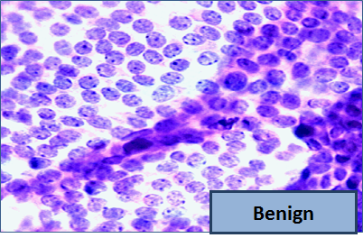
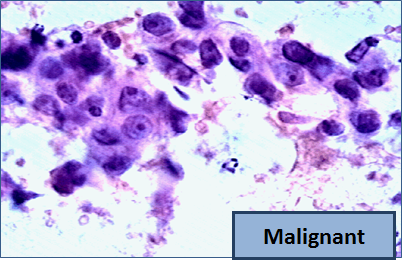
Unfortunately, distinguishing between benign vs malignant can be tricky. So, researchers have studied the use of machine learning to help with this task. The idea is that we’ll ask the lab tech to analyze the image and compute various attributes: things like the typical size of a cell, how much variation there is among the cell sizes, and so on. Then, we’ll try to use this information to predict (classify) whether the sample is malignant or not. We have a training set of past samples from women where the correct diagnosis is known, and we’ll hope that our machine learning algorithm can use those to learn how to predict the diagnosis for future samples.

We end up with the following data set. For the “Class” column, 1 means malignant (cancer); 0 means benign (not cancer).

Python

# Import data set breast-cancer.csv
url = "https://github.com/ZacksAmber/Code/raw/master/Data%20Science/Data8/Data%20Sets/breast-cancer.csv"
breast_cancer = pd.read_csv(url)

breast_cancer

	ID	Clump Thickness	Uniformity of Cell Size	Uniformity of Cell Shape	Marginal Adhesion	Single Epithelial Cell Size	Bare Nuclei	Bland Chromatin	Normal Nucleoli	Mitoses	Class
0	1000025	5	1	1	1	2	1	3	1	1	0
1	1002945	5	4	4	5	7	10	3	2	1	0
2	1015425	3	1	1	1	2	2	3	1	1	0
3	1016277	6	8	8	1	3	4	3	7	1	0
4	1017023	4	1	1	3	2	1	3	1	1	0
...	...	...	...	...	...	...	...	...	...	...	...
678	776715	3	1	1	1	3	2	1	1	1	0
679	841769	2	1	1	1	2	1	1	1	1	0
680	888820	5	10	10	3	7	3	8	10	2	1
681	897471	4	8	6	4	3	4	10	6	1	1
682	897471	4	8	8	5	4	5	10	4	1	1

So we have 9 different attributes. I don’t know how to make a 9-dimensional scatterplot of all of them, so I’m going to pick two and plot them:

Python

# 2-D Scatter plot
fig = go.Figure()

df = breast_cancer
label_x = 'Bland Chromatin'
label_y = 'Single Epithelial Cell Size'
cls = 'Class'
title = 'Scatter of Breast Cancer'

# Add trace label_x & label_y where cls == 1
fig.add_trace(go.Scatter(
    mode='markers',
    x=df[df[cls] == 1][label_x],
    y=df[df[cls] == 1][label_y],
    name=f'{cls}: 1',
    marker_color='rgba(2, 21, 51, .9)'))

# Add trace label_x & label_y where cls == 0
fig.add_trace(go.Scatter(
    mode='markers',
    x=df[df[cls] == 0][label_x],
    y=df[df[cls] == 0][label_y],
    name=f'{cls}: 0',
    marker_color='rgba(253, 188, 34, .9)'))

# Set layout
fig.update_layout(
    title=title,
    xaxis_title=label_x,
    yaxis_title=label_y,
    height=600,
    width=1200)

fig.show()
fig.write_image('fig.svg')
# ![](https://raw.githubusercontent.com/ZacksAmber/PicGo/master/img/20210624141250.svg)

Oops. That plot is utterly misleading, because there are a bunch of points that have identical values for both the x- and y-coordinates. To make it easier to see all the data points, I’m going to add a little bit of random jitter to the x- and y-values. Here’s how that looks:

Python

# 2-D Scatter plot
fig = go.Figure()

df = breast_cancer
label_x = 'Bland Chromatin'
label_y = 'Single Epithelial Cell Size'
cls = 'Class'
title = 'Scatter of Breast Cancer'

# Add trace label_x & label_y where cls == 1
fig.add_trace(go.Box(
    boxpoints = 'all', # plot all points
    jitter = 0.5,
    hoveron = 'points', 
    #pointpos = 0, # center the points on the x-axis
    fillcolor = 'rgba(255,255,255,0)', # hiding the whisker boxes
    line_color = 'rgba(255,255,255,0)', # hiding the whisker boxes
    showlegend = True,
    x=df[df[cls] == 1][label_x],
    y=df[df[cls] == 1][label_y],
    name=f'{cls}: 1',
    marker_color='rgba(2, 21, 51, .9)'))

# Add trace label_x & label_y where cls == 0
fig.add_trace(go.Box(
    boxpoints = 'all',
    jitter = 0.5,
    hoveron = 'points',
    pointpos = 0,
    fillcolor = 'rgba(255,255,255,0)',
    line_color = 'rgba(255,255,255,0)',
    showlegend = True,
    x=df[df[cls] == 0][label_x],
    y=df[df[cls] == 0][label_y],
    name=f'{cls}: 0',
    marker_color='rgba(253, 188, 34, .9)'))

# Set layout
fig.update_layout(
    title=title,
    xaxis_title=f'{label_x} (jittered)',
    yaxis_title=f'{label_y} (jittered)',
    height=600,
    width=1200)

fig.show()
fig.write_image('fig.svg')
# ![](https://raw.githubusercontent.com/ZacksAmber/PicGo/master/img/20210624153009.svg)

For instance, you can see there are lots of samples with chromatin = 2 and epithelial cell size = 2; all non-cancerous.

Keep in mind that the jittering is just for visualization purposes, to make it easier to get a feeling for the data. We’re ready to work with the data now, and we’ll use the original (unjittered) data.

First we’ll create a training set and a test set. The data set has 683 patients, so we’ll randomly permute the data set and put 342 of them in the training set and the remaining 341 in the test set.

Python

train, test = train_test_split(breast_cancer, test_size = 0.5)
attributes = ['Bland Chromatin', 'Single Epithelial Cell Size']
k = 5
cls = 'Class'

knn_breast_cancer = KNN(k=k, train=train, attributes=attributes, cls=cls)
best_k = knn_breast_cancer.best_k(test=test, repetition=100)

best_k

	k	Average Accuracy of 100 Boostrap
4	5	0.931637
2	3	0.926550
3	4	0.920058
0	1	0.904591
1	2	0.896287

Over 96% accuracy. Not bad! Once again, pretty darn good for such a simple technique.

As a footnote, you might have noticed that Brittany Wenger did even better. What techniques did she use? One key innovation is that she incorporated a confidence score into her results: her algorithm had a way to determine when it was not able to make a confident prediction, and for those patients, it didn’t even try to predict their diagnosis. Her algorithm was 99% accurate on the patients where it made a prediction – so that extension seemed to help quite a bit.

---

Multiple Regression

Now that we have explored ways to use multiple attributes to predict a categorical variable, let us return to predicting a quantitative variable. Predicting a numerical quantity is called regression, and a commonly used method to use multiple attributes for regression is called multiple linear regression.

---

IPython

Python

from IPython.display import YouTubeVideo
# The original URL is: 
# https://www.youtube.com/watch?v=U7db6ZeLR5s

YouTubeVideo("U7db6ZeLR5s")

---

Clustering

Visualizing K-Means algorithm with D3.js

Here is simpler steps:

1. Initialization: Create N nodes (circle) and randomly put initial K cluster (cross).
2. Assignment step: Assign each node (circle) to the nearest cluster (cross).
3. Update step: Each cluster (cross) move to the centroid of its nodes.
4. Go to step 2.

K-Means Clustering Explained Visually In 5 Minutes

A Complete Beginners Guide to Document Similarity Algorithms

---

Statistical functions (scipy.stats)

T-Test

A t-test is a type of inferential statistic used to determine if there is a significant difference between the means of two groups, which may be related in certain features. It is mostly used when the data sets, like the data set recorded as the outcome from flipping a coin 100 times, would follow a normal distribution and may have unknown variances. A t-test is used as a hypothesis testing tool, which allows testing of an assumption applicable to a population.

A t-test looks at the t-statistic, the t-distribution values, and the degrees of freedom to determine the statistical significance. To conduct a test with three or more means, one must use an analysis of variance.

KEY TAKEAWAYS

• A t-test is a type of inferential statistic used to determine if there is a significant difference between the means of two groups, which may be related in certain features.
• The t-test is one of many tests used for the purpose of hypothesis testing in statistics.
• Calculating a t-test requires three key data values. They include the difference between the mean values from each data set (called the mean difference), the standard deviation of each group, and the number of data values of each group.
• There are several different types of t-test that can be performed depending on the data and type of analysis required.

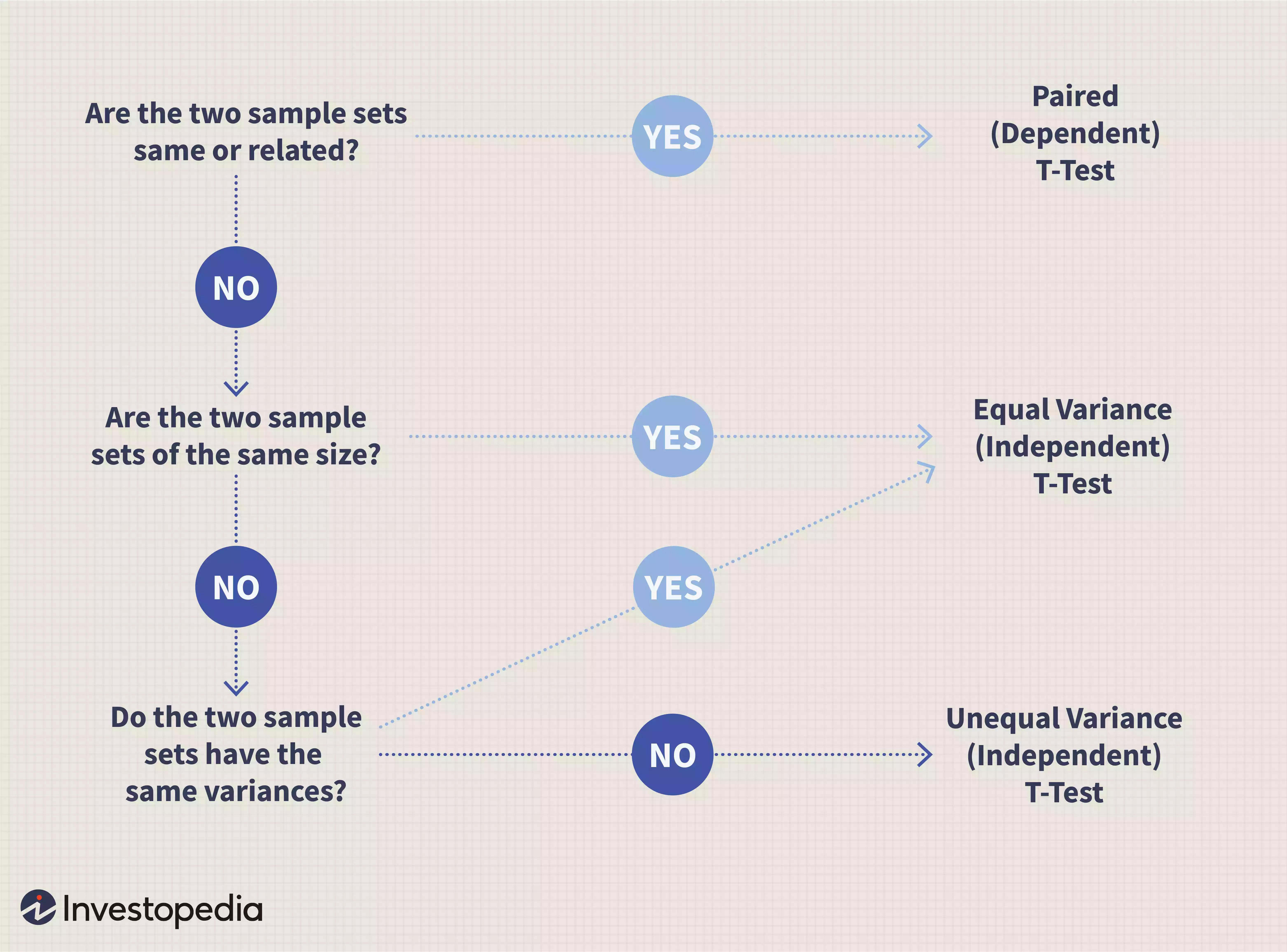
The T-test is a statistical test used to determine whether a numeric data sample of differs significantly from the population or whether two samples differ from one another.

One-Sample T-Test
A one-sample t-test checks whether a sample mean differs from the population mean.

Two-Sample T-Test
A two-sample t-test investigates whether the means of two independent data samples differ from one another. In a two-sample test, the null hypothesis is that the means of both groups are the same. Unlike the one sample-test where we test against a known population parameter, the two sample test only involves sample means.

Paired T-Test
The basic two sample t-test is designed for testing differences between independent groups. In some cases, you might be interested in testing differences between samples of the same group at different points in time. For instance, a hospital might want to test whether a weight-loss drug works by checking the weights of the same group patients before and after treatment. A paired t-test lets you check whether the means of samples from the same group differ.

---

Z-Test

Z-Test

A z-test is a statistical test used to determine whether two population means are different when the variances are known and the sample size is large. The test statistic is assumed to have a normal distribution, and nuisance parameters such as standard deviation should be known in order for an accurate z-test to be performed.

KEY TAKEAWAYS

• Z-test is a statistical test to determine whether two population means are different when the variances are known and the sample size is large.
• Z-test is a hypothesis test in which the z-statistic follows a normal distribution.
• A z-statistic, or z-score, is a number representing the result from the z-test.
• Z-tests are closely related to t-tests, but t-tests are best performed when an experiment has a small sample size.
• Z-tests assume the standard deviation is known, while t-tests assume it is unknown.

Frequently Asked Questions
What’s the Difference Between a T-Test and Z-Test?
Z-tests are closely related to t-tests, but t-tests are best performed when an experiment has a small sample size, less than 30. Also, t-tests assume the standard deviation is unknown, while z-tests assume it is known. If the standard deviation of the population is unknown, but the sample size is greater than or equal to 30, then the assumption of the sample variance equaling the population variance is made while using the z-test.

What Is Central Limit Theorem (CLT)?
In the study of probability theory, the central limit theorem (CLT) states that the distribution of sample approximates a normal distribution (also known as a “bell curve”) as the sample size becomes larger, assuming that all samples are identical in size, and regardless of the population distribution shape. Sample sizes equal to or greater than 30 are considered sufficient for the CLT to predict the characteristics of a population accurately.

What Is a Z-Score?
A z-score, or z-statistic, is a number representing how many standard deviations above or below the mean population the score derived from a z-test is. Essentially, it is a numerical measurement that describes a value’s relationship to the mean of a group of values. If a Z-score is 0, it indicates that the data point’s score is identical to the mean score. A Z-score of 1.0 would indicate a value that is one standard deviation from the mean. Z-scores may be positive or negative, with a positive value indicating the score is above the mean and a negative score indicating it is below the mean.

---

1. 1.Surprisingly, when we add infinitely many fractions, the order can matter! But our approximation to $\pi$ uses only a large finite number of fractions, so it’s okay to add the terms in any convenient order. ↩
2. 2.As we saw in the example about Leibniz’s formula, when we add infinitely many fractions, the order can matter. The same is true with multiplying fractions, as we are doing here. But our approximation to $\pi$ uses only a large finite number of fractions, so it’s okay to multiply the terms in any convenient order. ↩