A/B Testing
Introduction
When to run experiments
- Deciding whether or not to launch a new product or feature
- To quantify the impact of a feature or product
- Compare data with intuition. i.e. to better understand how users respond to certain parts of a product
Setting up an Experiment
- Define your goal and form your hypotheses.
- Identify a control and a treatment.
- Identify key metrics to measure.
- Identify what data needs to be controlled.
- Make sure that appropriate logging is in place to collect all necessary data.
- Determine how small of a difference you would like to detect.
- Determine what fraction of visitors you want to be in the treatment.
- Run a power analysis to decide how much data you need to collect and how long you need run the test.
- Run the test for AT LEAST this long.
- First time trying something new: run an A/A test (dummy test) simultaneously to check for systematic biases.
Case Studies
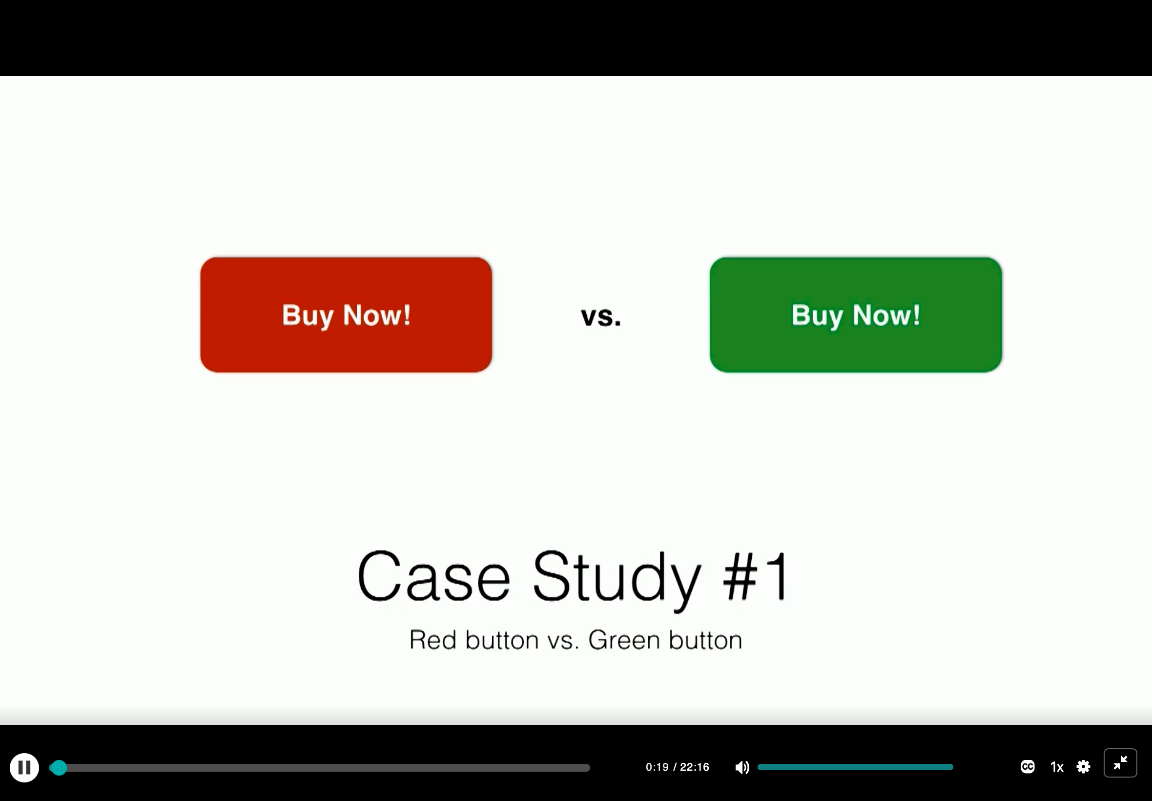
Red button Vs. Green Button
Step 1: Define goals and form hypotheses
Goal: Quantify the impact a different call-to-action button color has on metrics.
Hypotheses:
- Compared with a red CTA button, a green CTA button will entice users to click who would not have had otherwise.
- A fraction of these additional clickers will complete the transaction, increasing revenue.
- We expect the change in behavior to be most pronounced on mobile.
Null hypothesis:
- Green button will cause no difference in Click through rate or other user behavior
Step 2: Identify treatment & control
Control: Red button
Treatment: Green button
Step 3: Identify key metrics to measure
- Revenue
- Purchase rate: Purchases per visitor OR purchase per clicker
- Click through rate: Click per visit, OR clickers per visitor
- Other behavioral metrics
- Bounce rate
- Time on site
- Return visits
- Engagement with other parts of the website
- Referrals
- etc.
Step 4: Identify data to be collected
- User id (if the user is logged in)
- Cookie id
- What platform the visitor is on
- Page loads
- Experiment assignment
- If the user sees a button, and which color
- Clicks on the button, and which color
- Data for other metrics (ie engagement behavior)
Step 5: Make suer logging is in place
Smoke test everything!
- Does it work on mobile? How does it work if the user is logged out?
- What happens if you press the ‘back’ button?
- What happens if some other experiment is triggered as well?
- Does the logging interfere with any other logging?
Step 6: Determine how small of a difference needs to detected
Current button CTR: 3%
Successful experiment: 3.3% or more
This means that we would need to collect enough data to measure a 10% increase.
Step 7: Determine what fraction of visitors you want to be in the treatment
50/50 splits are the easiest and take the least amount of time to run, but you might no always want to do that.
A change will influence a lot. Before you gain enough evidence to prove a positive impact on your business, don’t make a huge change.
So maybe:
- Red button (original design): 90% of visitors
- Green button: 10% of visitors
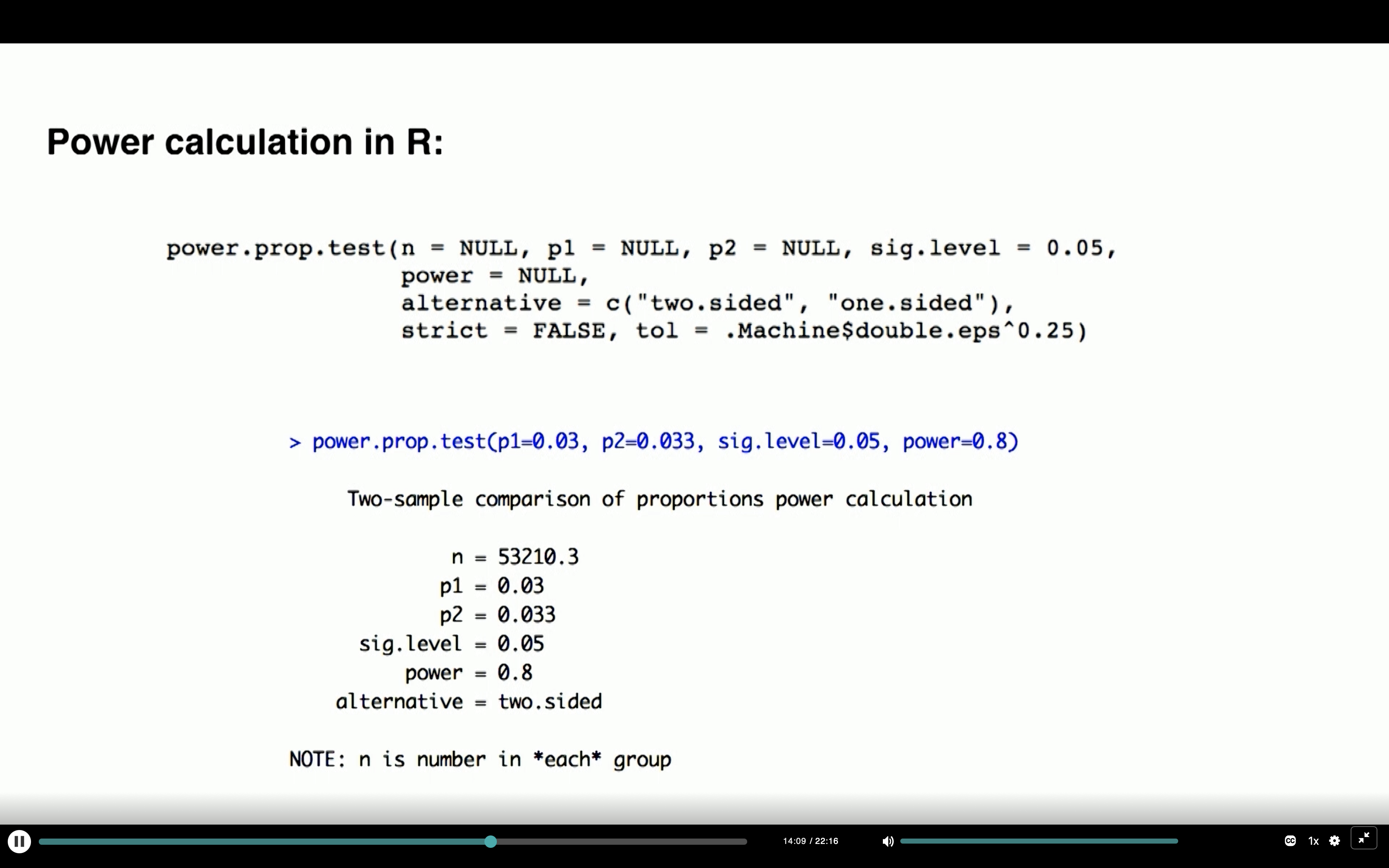
Step 8: Calculate how much data to collect and how long you need to run the experiment for
Run a power analysis to decide how many data samples to collect depending on your tolerance for:
Minimum measurable difference (10% in our case)
False negatives
False positives
Hypotheses:
- Compared with a red CTA button, a green CTA button will entice users to click who would not have had otherwise.
- A fraction of these additional clickers will complete the transaction, increasing revenue.
- We expect the change in behavior to be most pronounced on mobile.
Null hypothesis:
- Green button will cause no difference in Click through rate or other user behavior
| Table of error types | Null hypothesis (H0) is | ||
|---|---|---|---|
| True | False | ||
| Decision about null hypothesis (H0) |
Don't reject |
Correct inference (true negative) (probability = 1−α) |
Type II error (false negative) (probability = β) |
| Reject | Type I error (false positive) (probability = α) |
Correct inference (true positive) (probability = 1−β) | |
False positive (Type I error): We see a significant result (null hypothesis is false, but it should be true) when there isn’t one.
- Falsely reject the null hypothesis
- Typically, we want a false positive rate of < 5%: $\alpha = 0.05$
- False positive rate is equivalent ot the significance level of a statistical test.
False negative (Type II error): there is a an effect, but we weren’t able to measure it (null hypothesis is true, but it should be false).
- We should reject the null hypothesis, but don’t
- Typically, we want false negative rate to be < 20 %: $\beta = 0.2$
- The power of the test is $1 - \beta = 0.8$
The tolerance of Type II error is higher than Type I error.
Because it’s better to have a effect than no effect.
Higher accuracy means much more data to collect.
Step 9: Figure out how long to run the test and run test for AT LEAST that long
For 50/50 A/B test
We need at least 53,210 * 2 = 106,420 users
If our traffics ~ 100,000 unique users/day, we need to run the test for at least 1 day.
Note
If we were to run a 90/10 test, we should need 53,210 * 10 = 532,1000 users.
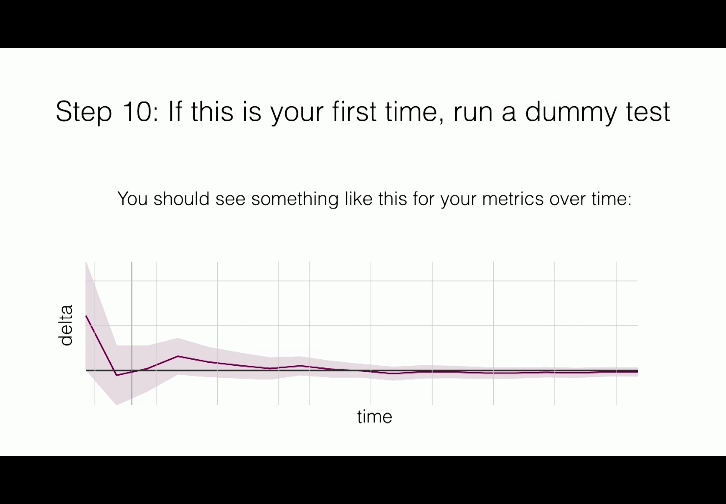
Step 10: If this is your first time, run a dummy test
A/A test: two groups, but no difference.
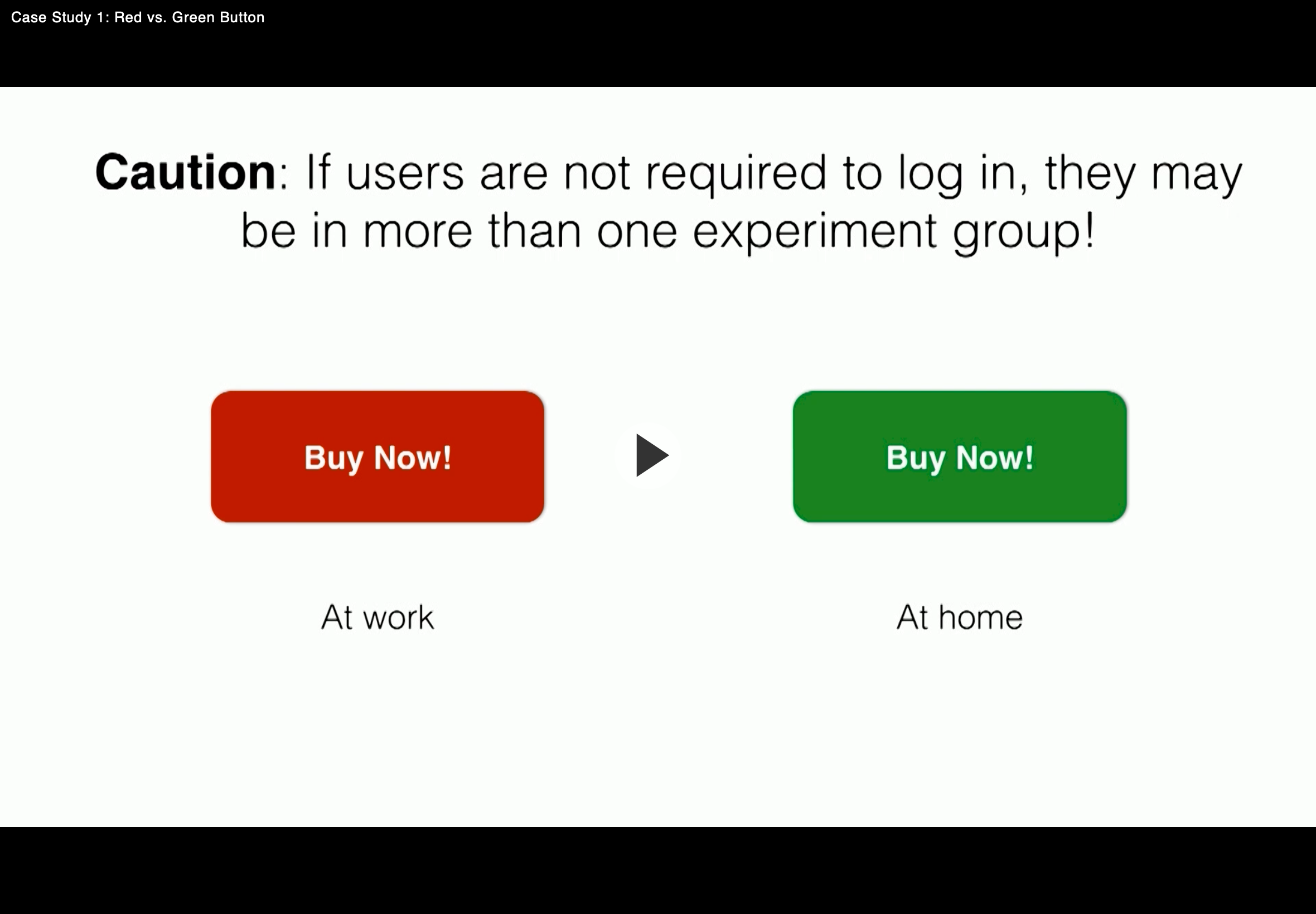
Cautions
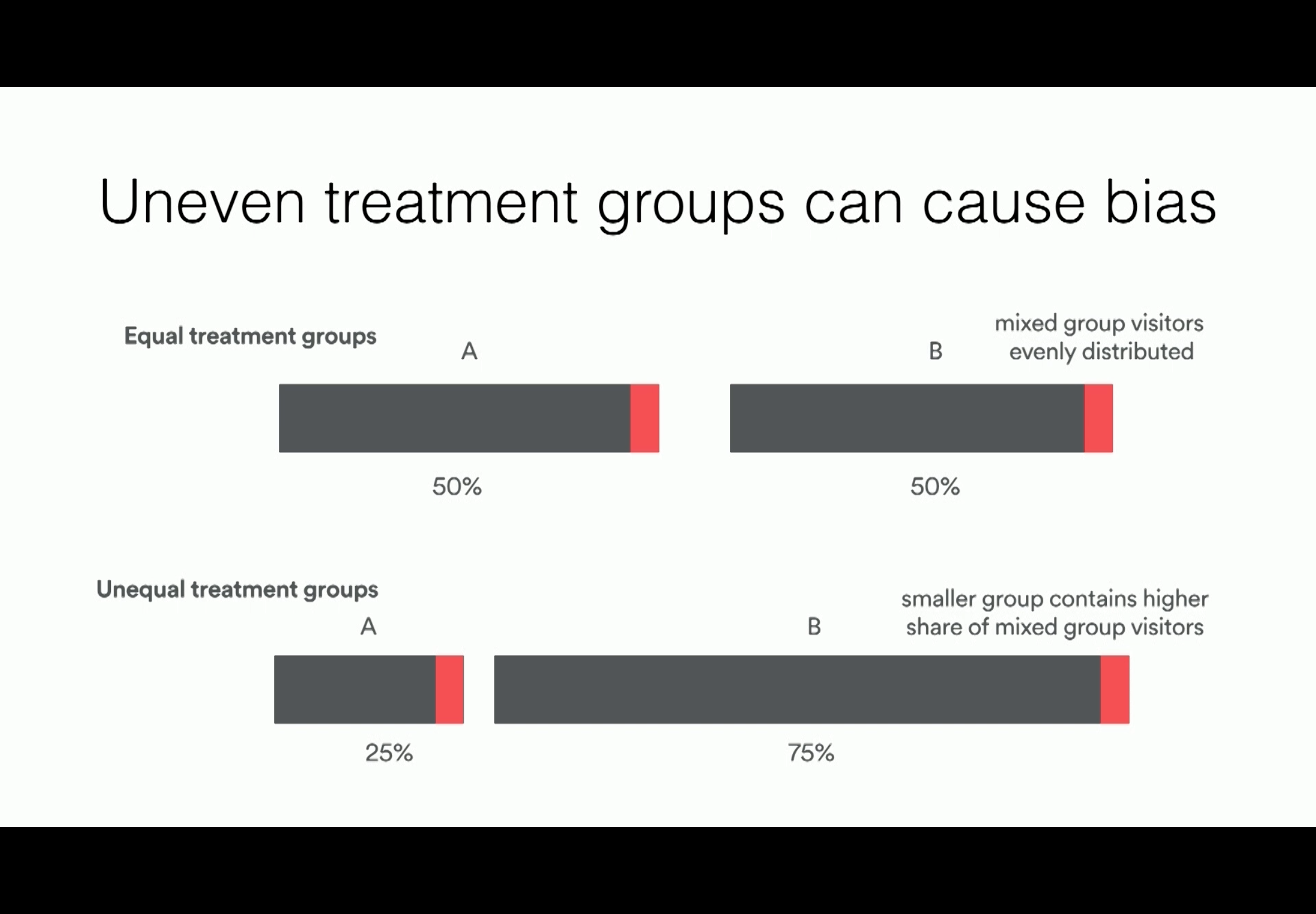
Caution: If users are not required to log in, they may be in more than one experiment group!
Uneven treatment groups can cause bias
Summary: Classic button color experiment
- Run a power analysis to determine how long to run test
- Don’t stop the test to early!
- If users do ont have to be logged in to be a part of the experiment, you can have problems with mixed group users.
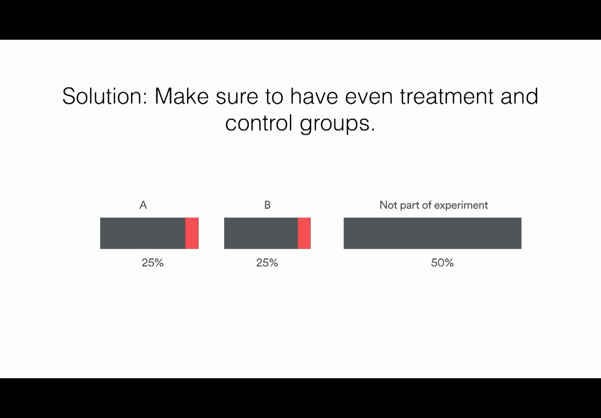
- To avoid systematic biases, suer that you have even treatment and control groups.
Testing a New Landing Page
Improve a boring page.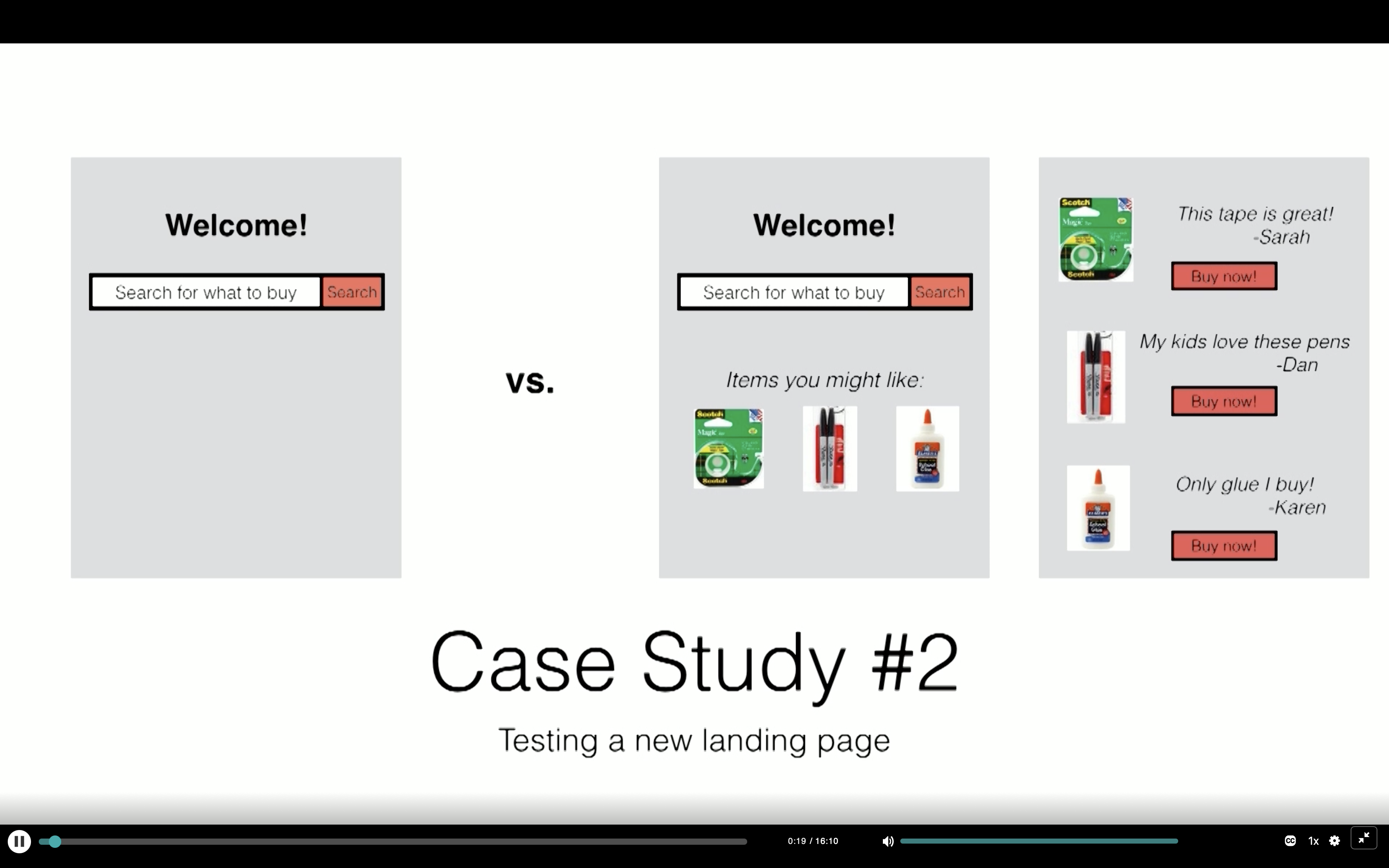
Step 1: Define goals and form hypotheses
Goal: Identify the impact of the new landing page and recommendation page on conversation and user behavior.
Hypotheses:
- Personalized suggestions aon homepage will engage visitors who should have otherwise bounced
- Relevant information on the next page will inspire visitors to make purchases who would not have otherwise.
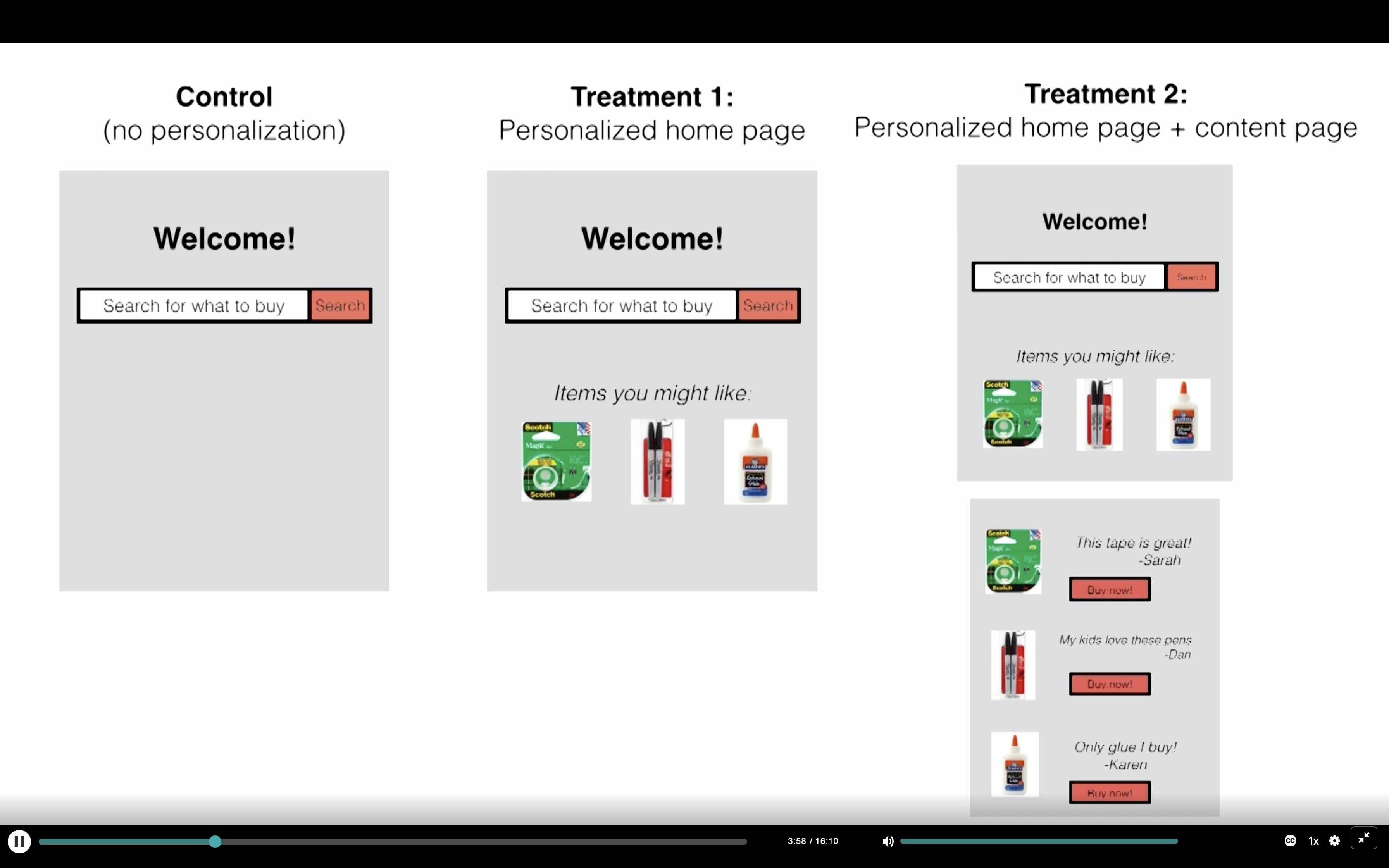
Step 2: Identify treatment & control
Control: Red button
Treatment: Green button
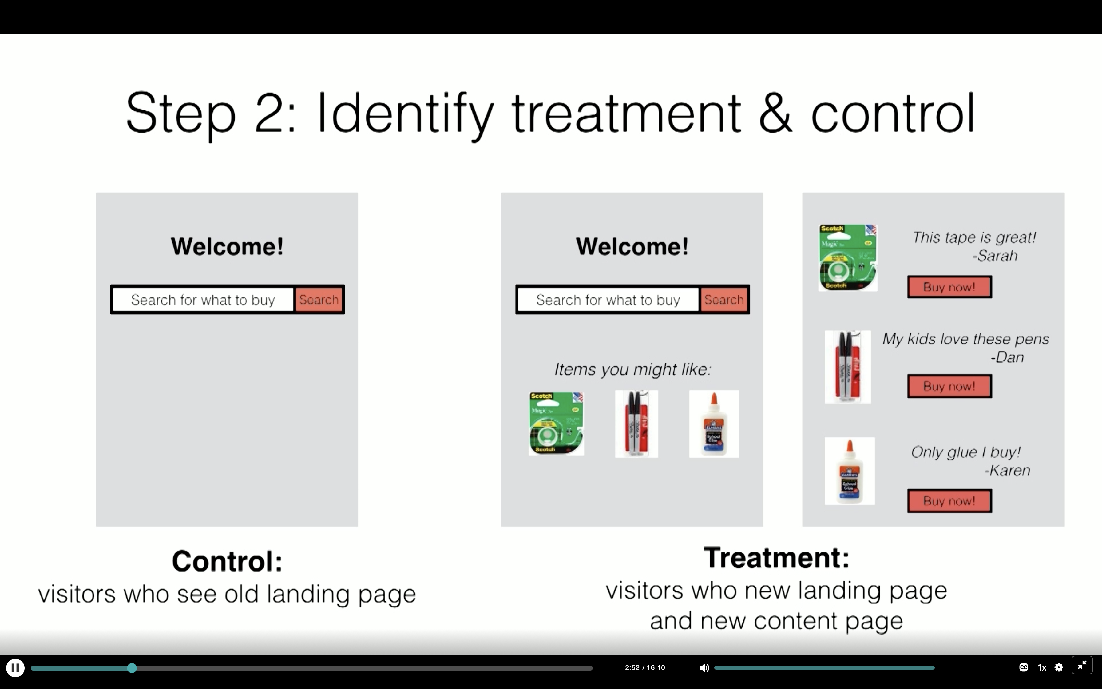
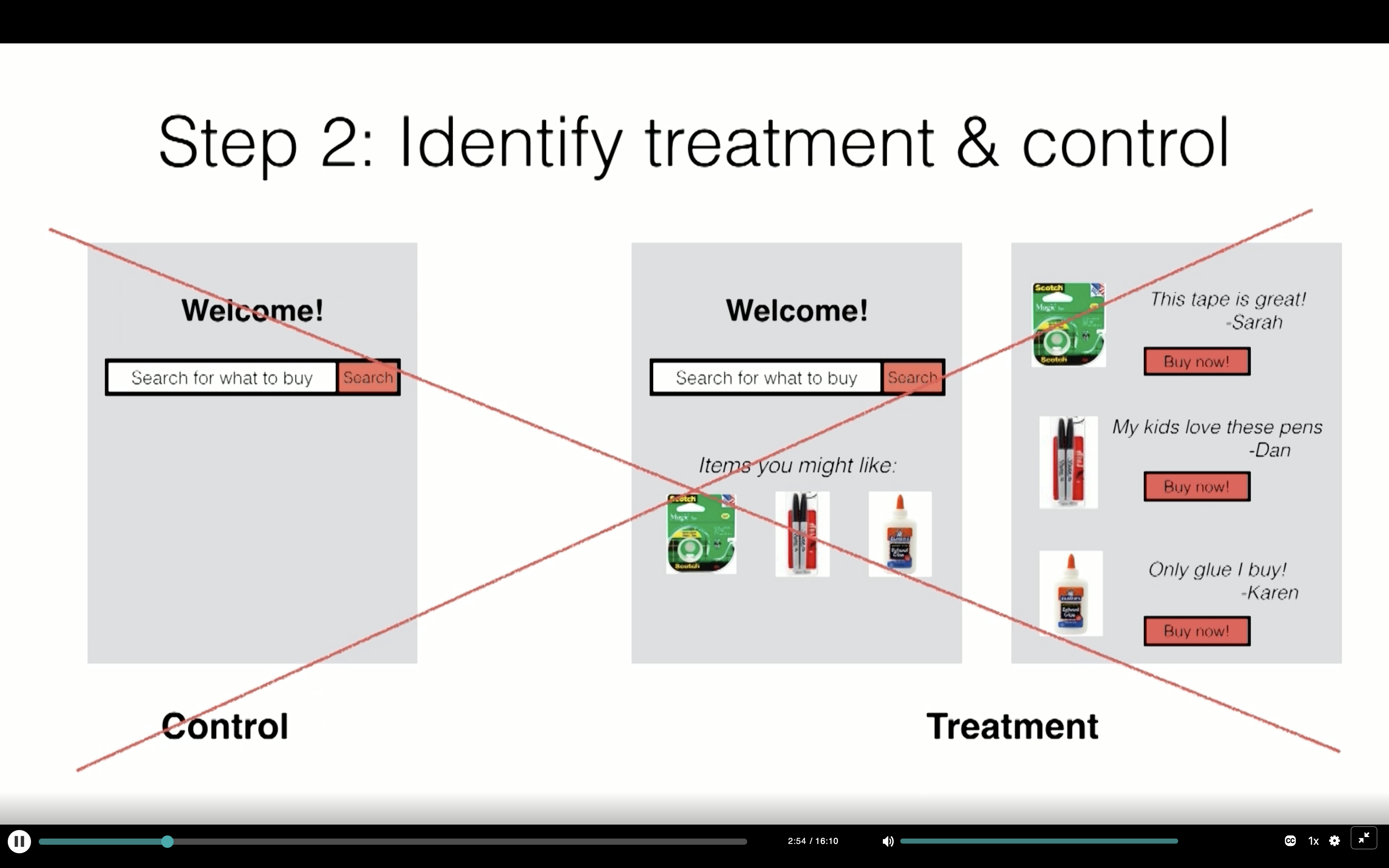
Tip: Only one thing should change between treatment and control
The above treatment has more pictures, more buttons, and more content. So you don’t know which one is the decisive factor.
Step 3: Identify key metrics to measure
- Between Control & Treatment 1: Bounce Rate on home page
- Between Treatment 1 & Treatment 2: Transactions
- Keep track of other metrics too for clues:
- Click through rates
- Searches
- Time on site
- etc.
Step 4: Identify data to be collected
- User id (if the user is logged in)
- Cookie id
- What platform the visitor is on
- Page loads
- Experiment assignment
- If they click on a recommendation and which one
- Any engagement on the content page
Step 5: Make suer logging is in place
Smoke test everything!
- Does it work on mobile? How does it work if the user is logged out?
- What happens if you press the ‘back’ button?
- What happens if some other experiment is triggered as well?
- Does the logging interfere with any other logging?
Step 6: Determine how small of a difference needs to detected
Current bounce rate: 50%
Successful experiment: 45% or less
Current transactions/visitor: 0.05
Successful experiment: 0.051
We want to be able to detect a 2% increase in transactions
Step 7: Determine what fraction of visitors you want to be in the treatment
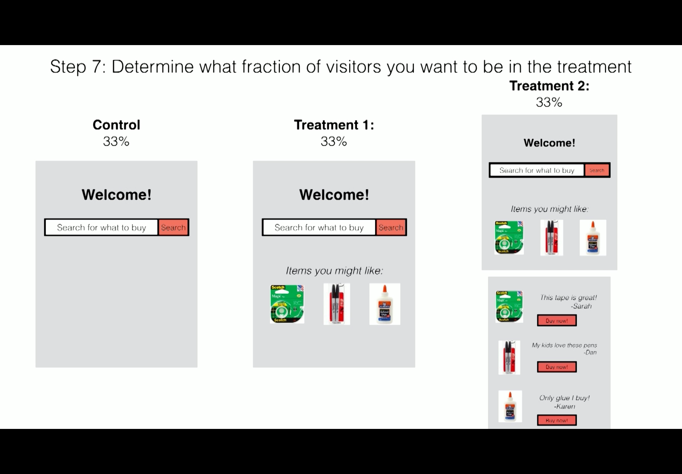
Since we have three groups, lets split everything evenly.
Step 8: Calculate how much data to collect
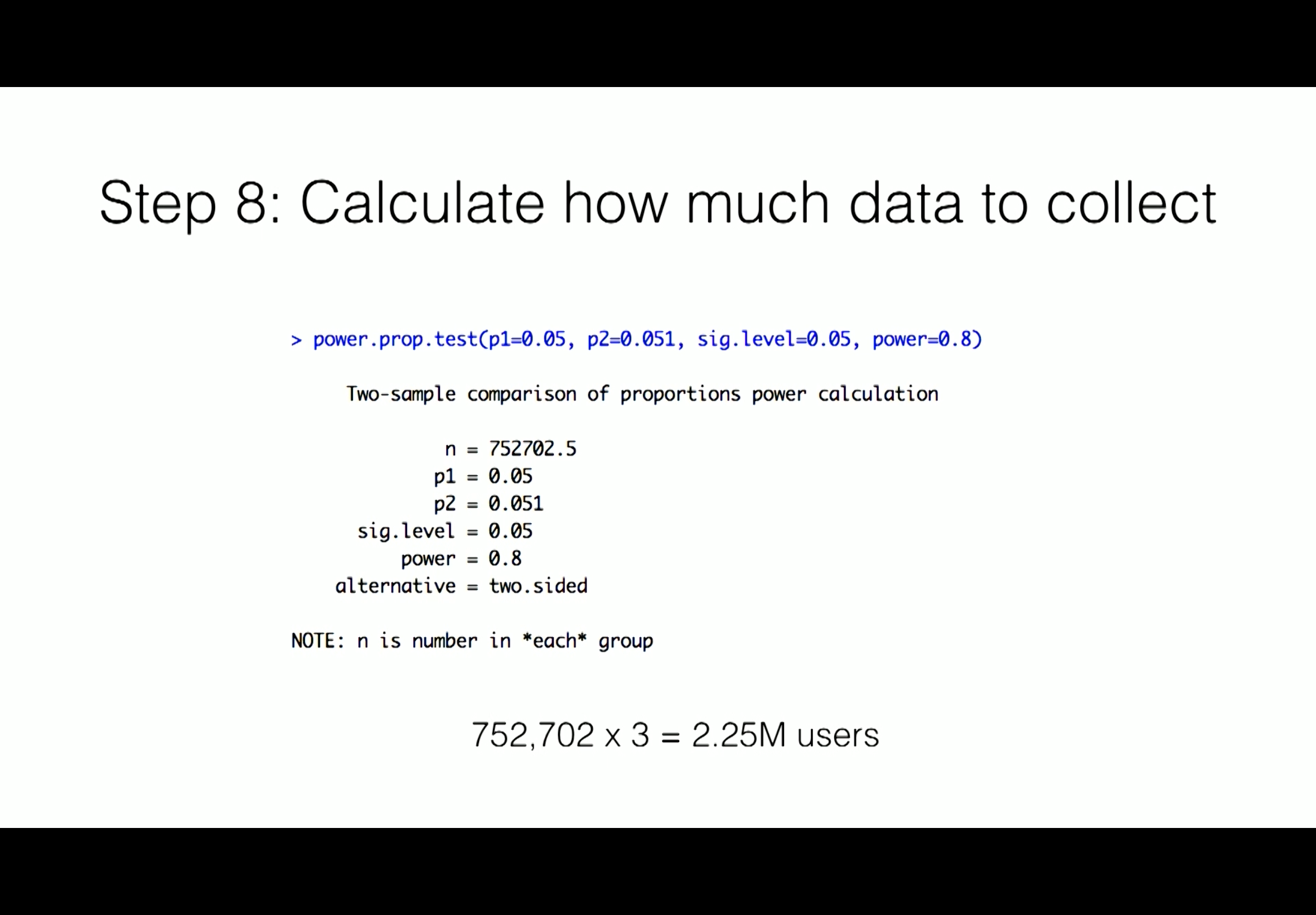
Higher accuracy means more population.
Step 9: Figure out how long to run the test and run test for AT LEAST that long
For $\alpha = 0.05$
We need at least 2.25M users.
If our traffic ~ 100,000 unique users/day, we need to run the test for at least 22.5 days.
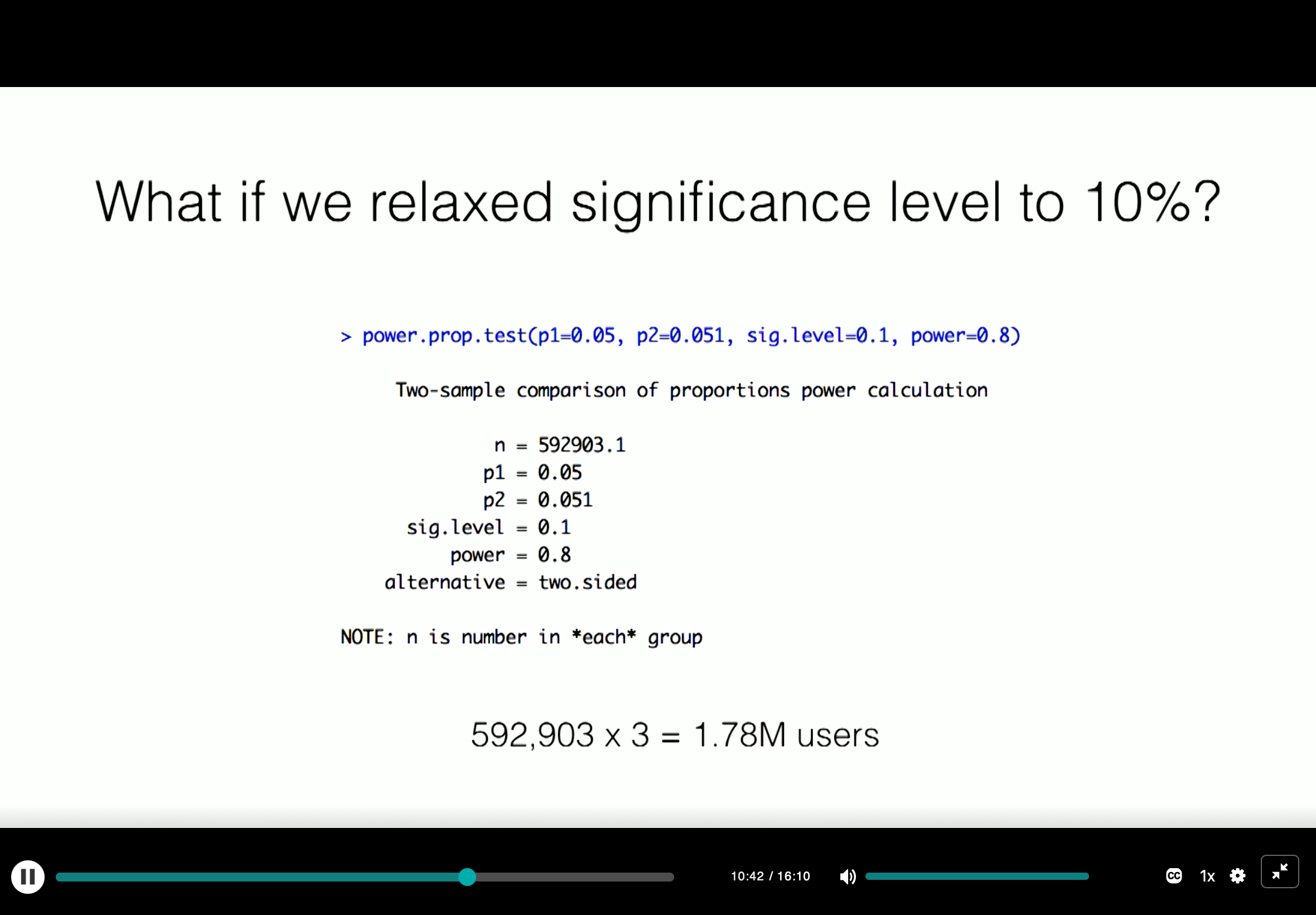
For $\alpha = 0.1$
We need at least 1.78M users.
If our traffic ~ 100,000 unique users/day, we need to run the test for at least 18 days.
Step 10: If this is your first time running a 3-way test, run a simultaneous dummy test
Bonus: Multi-armed bandit approach
Problem: We want to find the best variant, so we are willing to let the experiment run for longer. But we also want to maximize revenue during this experiment period.
Solution: Adjust fraction of (new) users in treatment/control according to which group seems to be doing better.
Summary: Landing page experiment
- Make sure only one thing changes between treatment and control
- Run another arm if necessary
A/B Testing from Google
Overview of A/B Testing
- Choose a metric
- Review statistics
- Design
- Analyze
Short
Small scale
treatment group and control group
Customer funnel
A:
- Click 0
- Visit 0
B:
- Click 5
- Visit 1 and reload 1
Click-through-Rate: Number of clicks / Number of page views
- 5/2
Click-through-Probability: Unique visitors who click / Unique visitors to page - 1/2
rate -> usability
- because users have variety of different places on the page that they can actually choose to click on
probability -> impact - because you don’t want to count users just double-clicked, or did they reload, or all of those types of issues
expected probability $\hat p = \frac{X}{N}$
- 100/1000 = 0.1
So the CI is 0.1.
To use normal:
- check $N \times \hat p > 5$
- and check $N \times (1- \hat p) > 5$
Margin of Error: the width away from CI
- $m = Z \times SE = Z \times \sqrt{\frac{\hat p (1 - \hat p)}{N}}$
For CL = 95%, Z = 1.96/-1.96
So m = 1.96 * np.sqrt(0.9 * (1-0.9)/1000) = 0.019
0.081 -> 0.1 -> 0.119
Two-tailed vs. one-tailed tests
The null hypothesis and alternative hypothesis proposed here correspond to a two-tailed test, which allows you to distinguish between three cases:
- A statistically significant positive result
- A statistically significant negative result
- No statistically significant difference.
Sometimes when people run A/B tests, they will use a one-tailed test, which only allows you to distinguish between two cases:
- A statistically significant positive result
- No statistically significant result
Which one you should use depends on what action you will take based on the results. If you’re going to launch the experiment for a statistically significant positive change, and otherwise not, then you don’t need to distinguish between a negative result and no result, so a one-tailed test is good enough. If you want to learn the direction of the difference, then a two-tailed test is necessary.
$\alpha = P(\mbox{reject null | null true})$
$\beta = P(\mbox{failed to reject | null false})$
Small sample:
- $\alpha$ low
- $\beta$ high
Large sample:
- $\alpha$ same
- $\beta$ low
1 - $\beta$ = sensitivity, often 80%
- Practical Significance, since it beyond $d_{min}$
- Neutral, since it includes zero, and no practically significant change.
- Statical Significance, a positive change, but no Practical Significance
- Neutral? It would be better to say that you do not have enough power to draw a strong conclusion. Running an additional test with greater power would be recommended in this situation.
- The point estimate ($\hat d$) is beyond what’s practically significant. But the CI overlaps 0, so there might not even be a change at all. It could potentially have no effect, so we cannot assume that is a positive change.
- Practical Significance. However, it’s also possible your change is no practically significant. Running an additional test with greater power if you have the time.
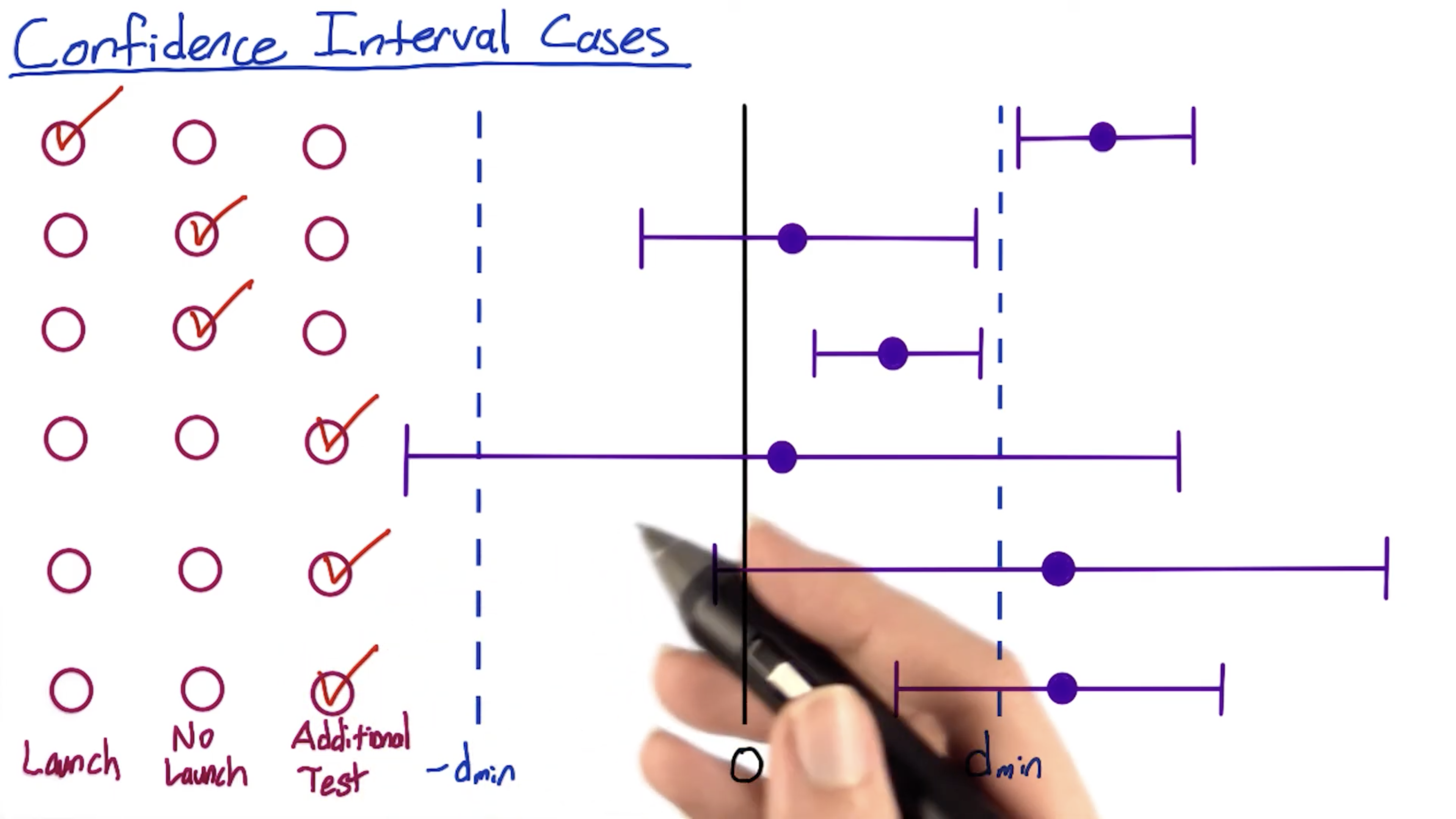
If one of the last three cases comes up and we don’t have time to run a new experiment, what we have to do is to communicate to the decision-makers when they’re going to have to make judgement, and take a risk. Because the data is uncertain. They’re going to have to use other factors, like strategic business issues, or other factors besides the data.
Policy and Ethics for Experiments
Four Principles of IRB’s
First Principle: Risk
First, in the study, what risk is the participant undertaking? The main threshold is whether the risk exceeds that of “minimal risk”. Minimal risk is defined as the probability and magnitude of harm that a participant would encounter in normal daily life. The harm considered encompasses physical, psychological and emotional, social, and economic concerns. If the risk exceeds minimal risk, then informed consent is required. We’ll discuss informed consent further below.
In most, but not all, online experiments, it can certainly be debated as to whether any of the experiments lead to anything beyond minimal risk. What risk is a participant going to be exposed to if we change the ranking of courses on an educational site, or if we change the UI on an online game?
Exceptions would certainly be any websites or applications that are health or financial related. In the Facebook experiment, for example, it can be debated as to whether participants were really being exposed to anything beyond minimal risk: all items shown were going to be in their feed anyway, it’s only a question of whether removing some of the posts led to increased risk.
Second Principle: Benefits
Next, what benefits might result from the study? Even if the risk is minimal, how might the results help? In most online A/B testing, the benefits are around improving the product. In other social sciences, it is about understanding the human condition in ways that might help, for example in education and development. In medicine, the risks are often higher but the benefits are often around improved health outcomes.
It is important to be able to state what the benefit would be from completing the study.
Third Principle: Alternatives
Third, what other choices do participants have? For example, if you are testing out changes to a search engine, participants always have the choice to use another search engine. The main issue is that the fewer alternatives that participants have, the more issue that there is around coercion and whether participants really have a choice in whether to participate or not, and how that balances against the risks and benefits.
For example, in medical clinical trials testing out new drugs for cancer, given that the other main choice that most participants face is death, the risk allowable for participants, given informed consent, is quite high.
In online experiments, the issues to consider are what the other alternative services that a user might have, and what the switching costs might be, in terms of time, money, information, etc.
Fourth Principle: Data Sensitivity
Finally, what data is being collected, and what is the expectation of privacy and confidentiality? This last question is quite nuanced, encompassing numerous questions:
- Do participants understand what data is being collected about them?
- What harm would befall them should that data be made public?
- Would they expect that data to be considered private and confidential?
For example, if participants are being observed in a public setting (e.g., a football stadium), there is really no expectation of privacy. If the study is on existing public data, then there is also no expectation of further confidentiality.
If, however, new data is being gathered, then the questions come down to:
- What data is being gathered? How sensitive is it? Does it include financial and health data?
- Can the data being gathered be tied to the individual, i.e., is it considered personally identifiable?
- How is the data being handled, with what security? What level of confidentiality can participants expect?
- What harm would befall the individual should the data become public, where the harm would encompass health, psychological / emotional, social, and financial concerns?
For example, often times, collected data from observed “public” behavior, surveys, and interviews, if the data were not personally identifiable, would be considered exempt from IRB review (reference: NSF FAQ below).
To summarize, there are really three main issues with data collection with regards to experiments:
- For new data being collected and stored, how sensitive is the data and what are the internal safeguards for handling that data? E.g., what access controls are there, how are breaches to that security caught and managed, etc.?
- Then, for that data, how will it be used and how will participants’ data be protected? How are participants guaranteed that their data, which was collected for use in the study, will not be used for some other purpose? This becomes more important as the sensitivity of the data increases.
- Finally, what data may be published more broadly, and does that introduce any additional risk to the participants?
Difference between pseudonymous and anonymous data
One question that frequently gets asked is what the difference is between identified, pseudonymous, and anonymous data is.
Identified data means that data is stored and collected with personally identifiable information. This can be names, IDs such as a social security number or driver’s license ID, phone numbers, etc. HIPAA is a common standard, and that standard has 18 identifiers (see the Safe Harbor method) that it considers personally identifiable. Device id, such as a smartphone’s device id, are considered personally identifiable in many instances.
Anonymous data means that data is stored and collected without any personally identifiable information. This data can be considered pseudonymous if it is stored with a randomly generated id such as a cookie that gets assigned on some event, such as the first time that a user goes to an app or website and does not have such an id stored.
In most cases, anonymous data still has time-stamps – which is one of the HIPAA 18 identifiers. Why? Well, we need to distinguish between anonymous data and anonymized data. Anonymized data is identified or anonymous data that has been looked at and guaranteed in some way that the re-identification risk is low to non-existent, i.e., that given the data, it would be hard to impossible for someone to be able to figure out which individual this data refers to. Often times, this guarantee is done statistically, and looks at how many individuals would fall into every possible bucket (i.e., combination of values).
What this means is that anonymous data may still have high re-identification risk (see AOL example).
So, if we go back to the data being gathered, collected, stored, and used in the experiment, the questions are:
- How sensitive is the data?
- What is the re-identification risk of individuals from the data?
As the sensitivity and the risk increases, then the level of data protection must increase: confidentiality, access control, security, monitoring & auditing, etc.
Additional reading
Daniel Solove’s “A Taxonomy of Privacy“ classifies some of things people mean by privacy in order to better understand privacy violations.
Summary of Principles
Summary: it is a grey area as to whether many of these Internet studies should be subject to IRB review or not and whether informed consent is required. Neither has been common to date.
Most studies, due to the nature of the online service, are likely minimal risk, and the bigger question is about data collection with regards to identifiability, privacy, and confidentiality / security. That said, arguably, a neutral third party outside of the company should be making these calls rather than someone with a vested interest in the outcome. One growing risk in online studies is that of bias and the potential for discrimination, such as differential pricing and whether that is discriminatory to a particular population for example. Discussing those types of biases is beyond the scope of this course.
Our recommendation is that there should be internal reviews of all proposed studies by experts regarding the questions:
- Are participants facing more than minimal risk?
- Do participants understand what data is being gathered?
- Is that data identifiable?
- How is the data handled?
And if enough flags are raised, that an external review happen.
Internal process recommendations
Finally, regarding internal process of data handling, we recommend that:
- Every employee who might be involved in A/B test be educated about the ethics and the protection of the participants. Clearly there are other areas of ethics beyond what we’ve covered that discuss integrity, competence, and responsibility, but those generally are broader than protecting participants of A/B tests (cite ACM code of ethics).
- All data, identified or not, be stored securely, with access limited to those who need it to complete their job. Access should be time limited. There should be clear policies of what data usages are acceptable and not acceptable. Moreover, all usage of the data should be logged and audited regularly for violations.
- You create a clear escalation path for how to handle cases where there is even possibly more than minimal risk or data sensitivity issues.
Additional Reading:
- Belmont Report
- Common Rule definition
- NSF guidelines
- NSF FAQ for Social Science & Behavioural research
- HHS IRB Guidebook
- UTexas overview
- UC Irvine overview
- The Association for Computer Machinery has developed a code of ethics.
- As an example, there’s a thorough outline of an “ideal” ethical privacy design for mobile connectivity measurements that could be used as a model.
Choosing and Characterizing Metrics
Metrics for Experiments
- Define
- Build Intuition
- Characterize
Metrics
- Invariant checking
- Sanity checking
- Evaluation Metrics
Metric Definition
Metrics: To measure whether the experiment group is better than the control group or not.
High Level Metrics: Customer Funnel
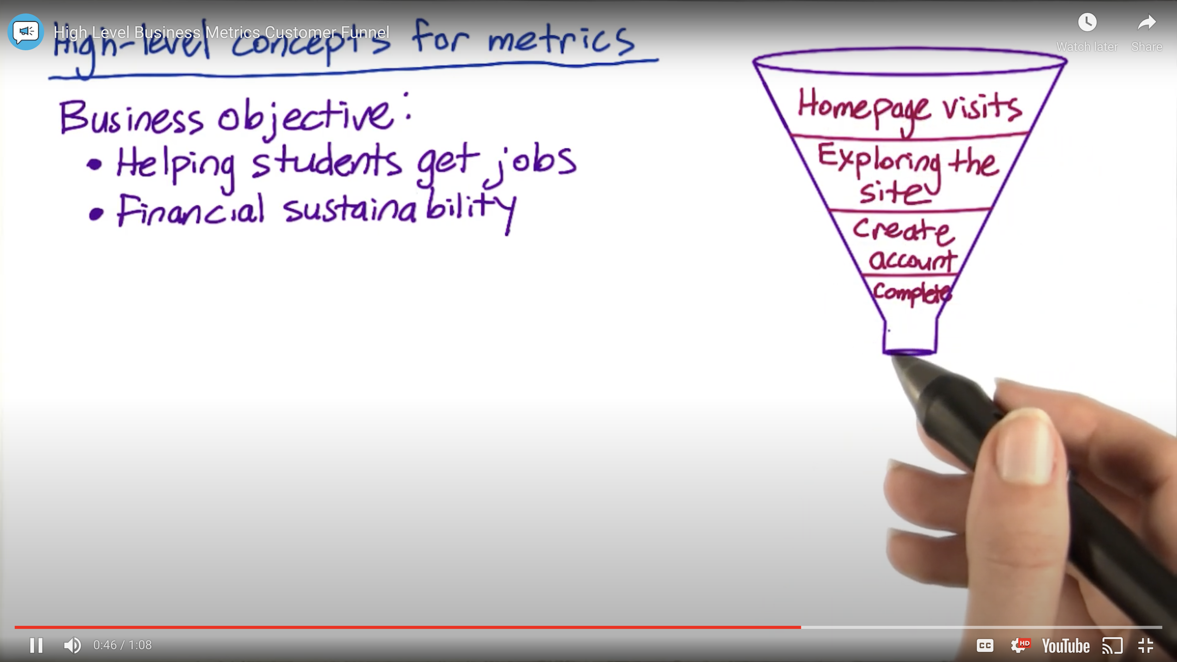
One metric, multiple metrics, or an OEC?
Objective Function or OEC (overall evaluation criterion): a composite metric to summarize all individual metrics
- Very tricky to let everyone agree with an OEC
Difficult metrics
- Don’t have access to data
- Takes too long
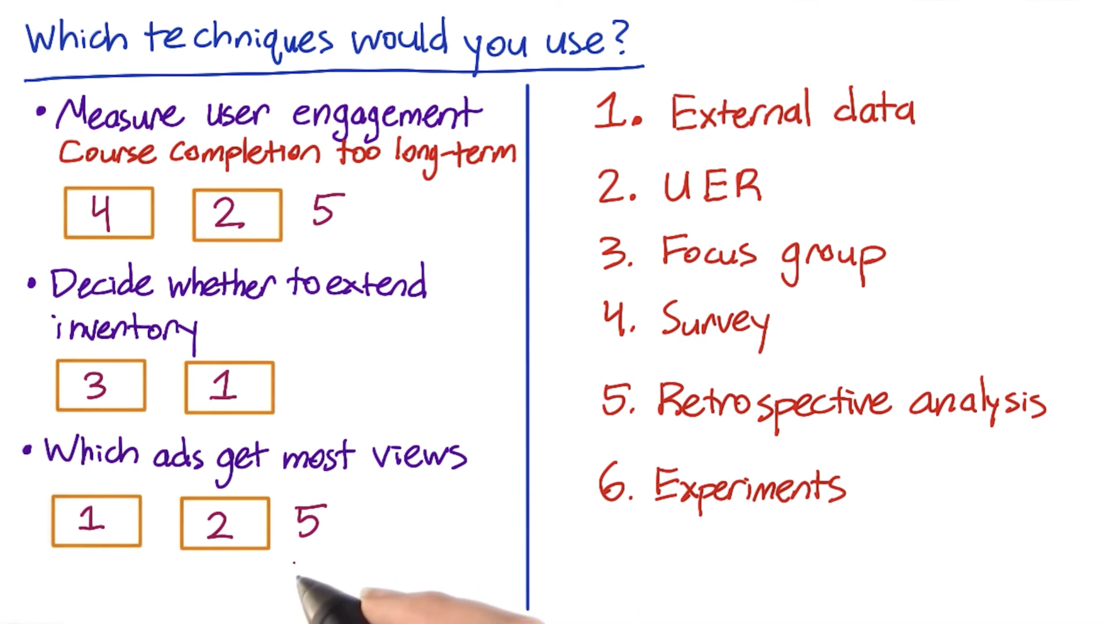
Additional techniques for difficultly defining metrics
External data
- Media measurement and analytics companies that providing marketing data and analytics to enterprises, like comScore or Nielsen
- Market research companies like Pew or Forrester
- Academic research, e.g, eye tracking. How much time do people stay on the page versus how long did it take them to actually click-through to the next page
Internal existing data
- retrospective (or observational) analyses
- surveys
- focus groups
Focus on your companies culture and requirements to make metrics:
- Some companies do not need to attract more visitors through website; While others do care.
- Some companies only want to make existing users happier.
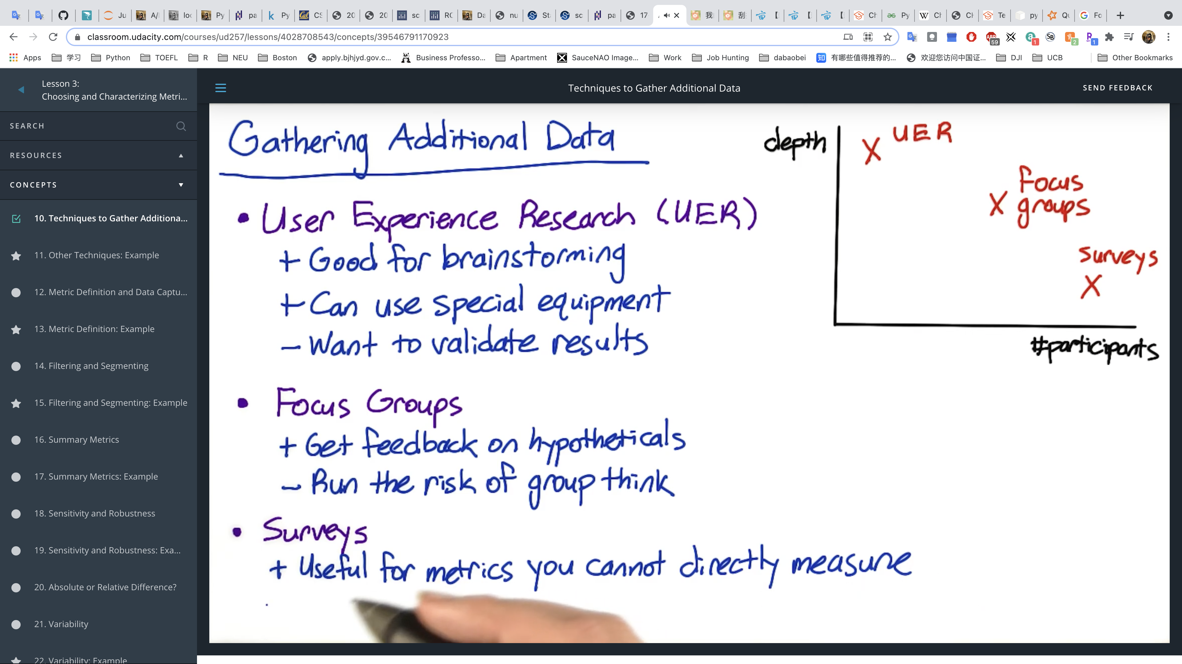
Relationship between participants and depth
- User Experience Research (UER)
- Good for brainstorming
- Can use special equipment, such as Eye-tracking cameras (Tobii)
- Want to validate results
- Focus Groups
- Get feed back on hypotheticals
- Run the risk of group think
- Surveys
- Useful for metrics you cannot directly measure
- Answers may not be truth
- Can’t directly compare to other results
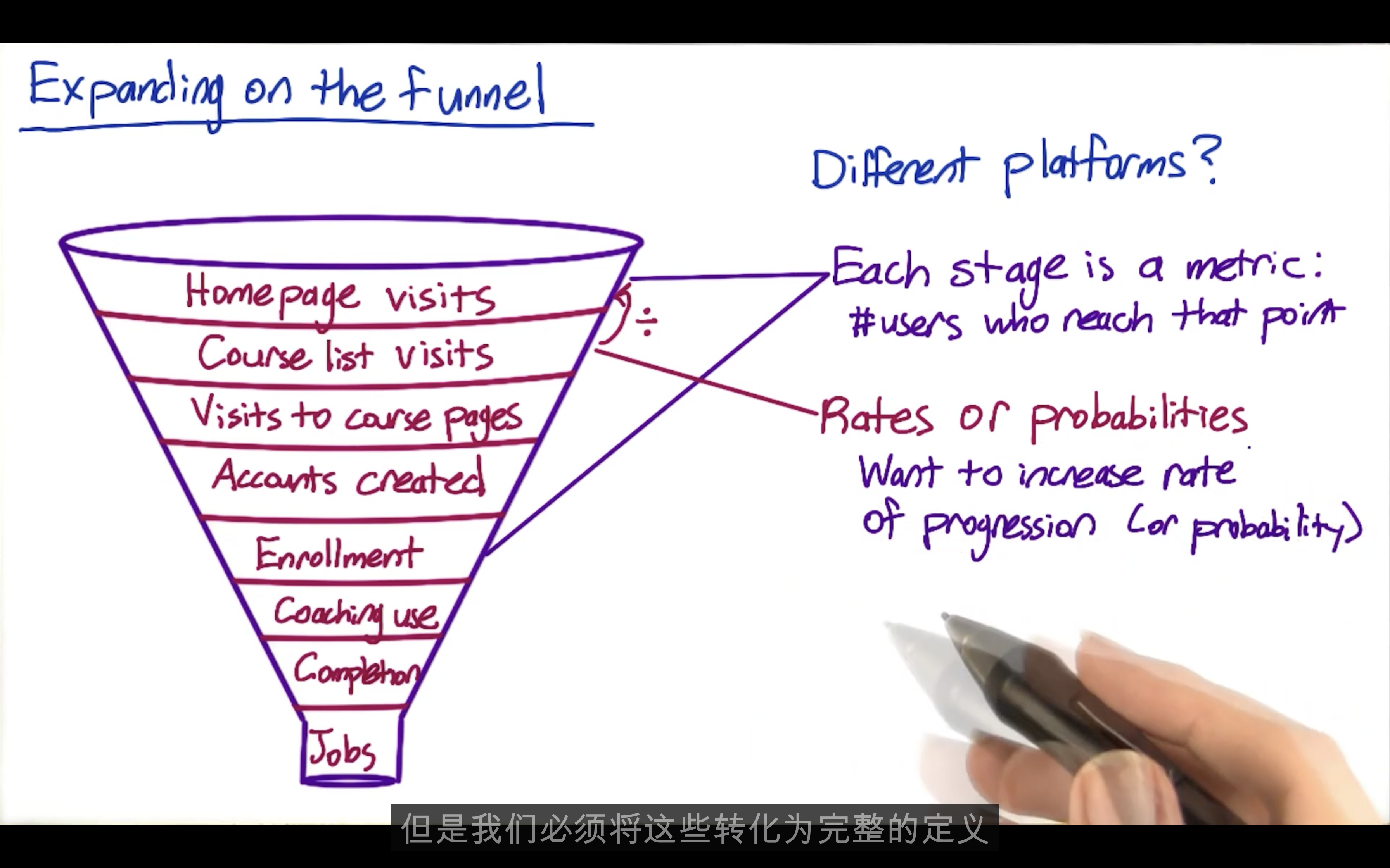
Metric Definition and Data Capture
To move from high level metrics to a fully realized definition:
- To fully define exactly what data will be used to calculate
- How to summarize the metrics
Working with engineering team to understand the data cross different platforms, such as click-through rate in Safari and IE are different.
Example
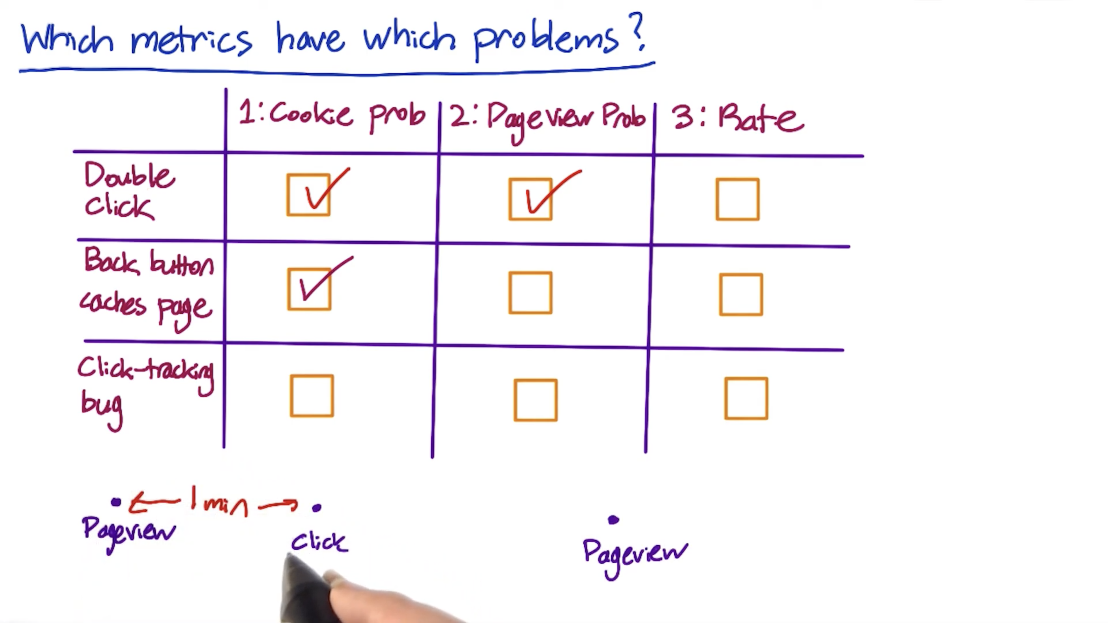
Defining a metric
Hight-level metric: Click-through-probability = #Users who click / #Users who visit
Def #1 (Cookie probability): For each
Click -> 5min -> reload but no click -> 30 sec -> reload and click -> 12 hr -> reload but no click
per minute: 2/3
per hour: 1/2
per day: 1
Def #2 (Pageview probability): Number of pageviews with a click within
pageview no click -> 30 sec -> refresh -> 1 sec -> click
Def #3 (Rate): Number of clicks divided by number of pageviews
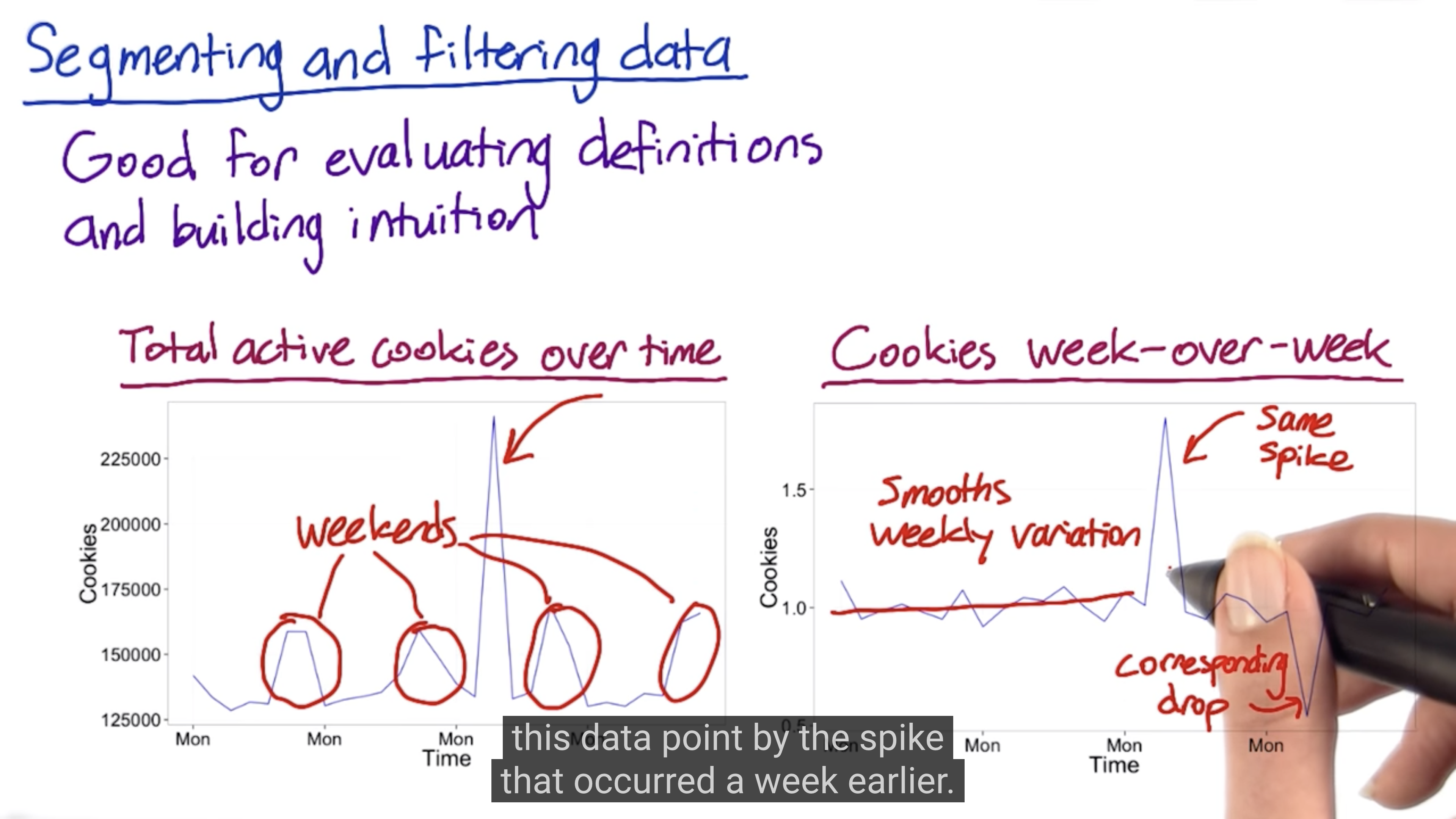
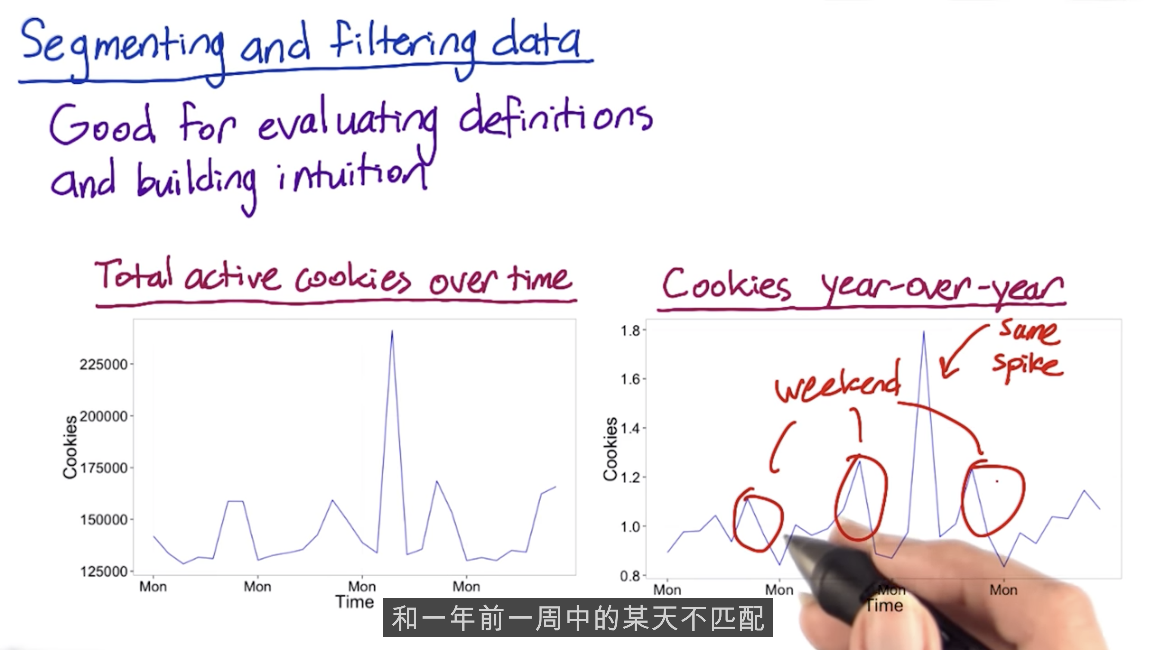
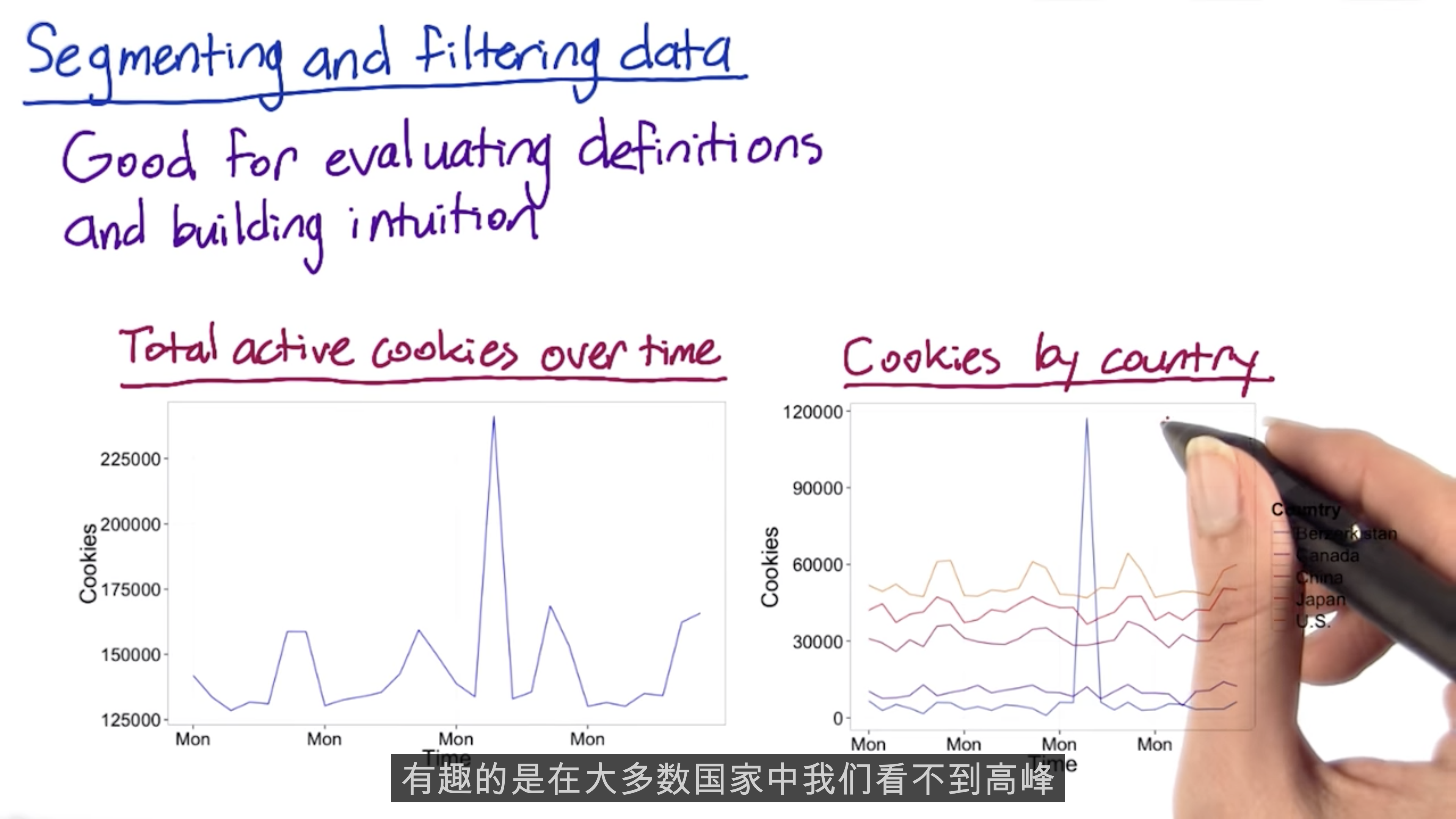
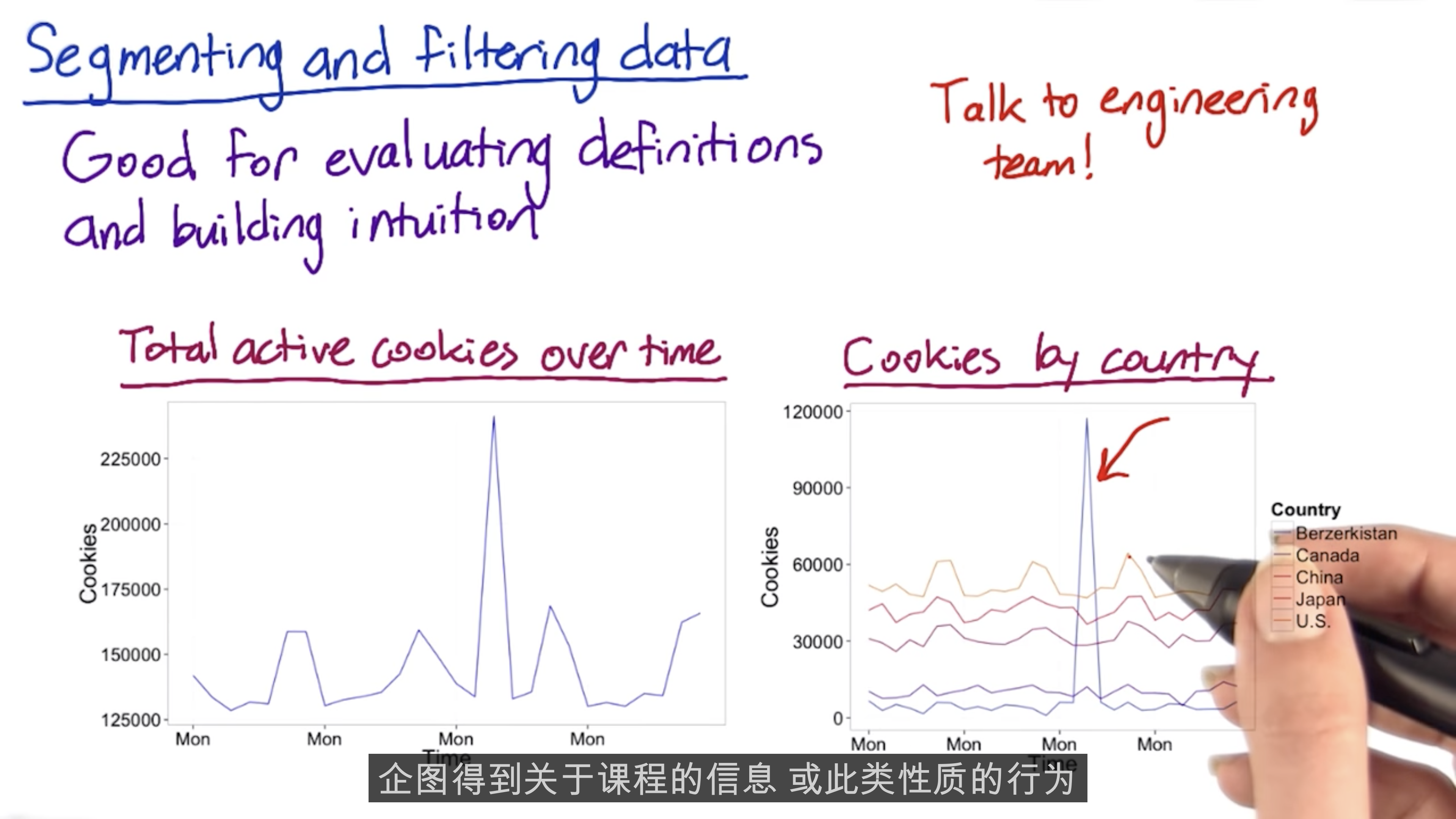
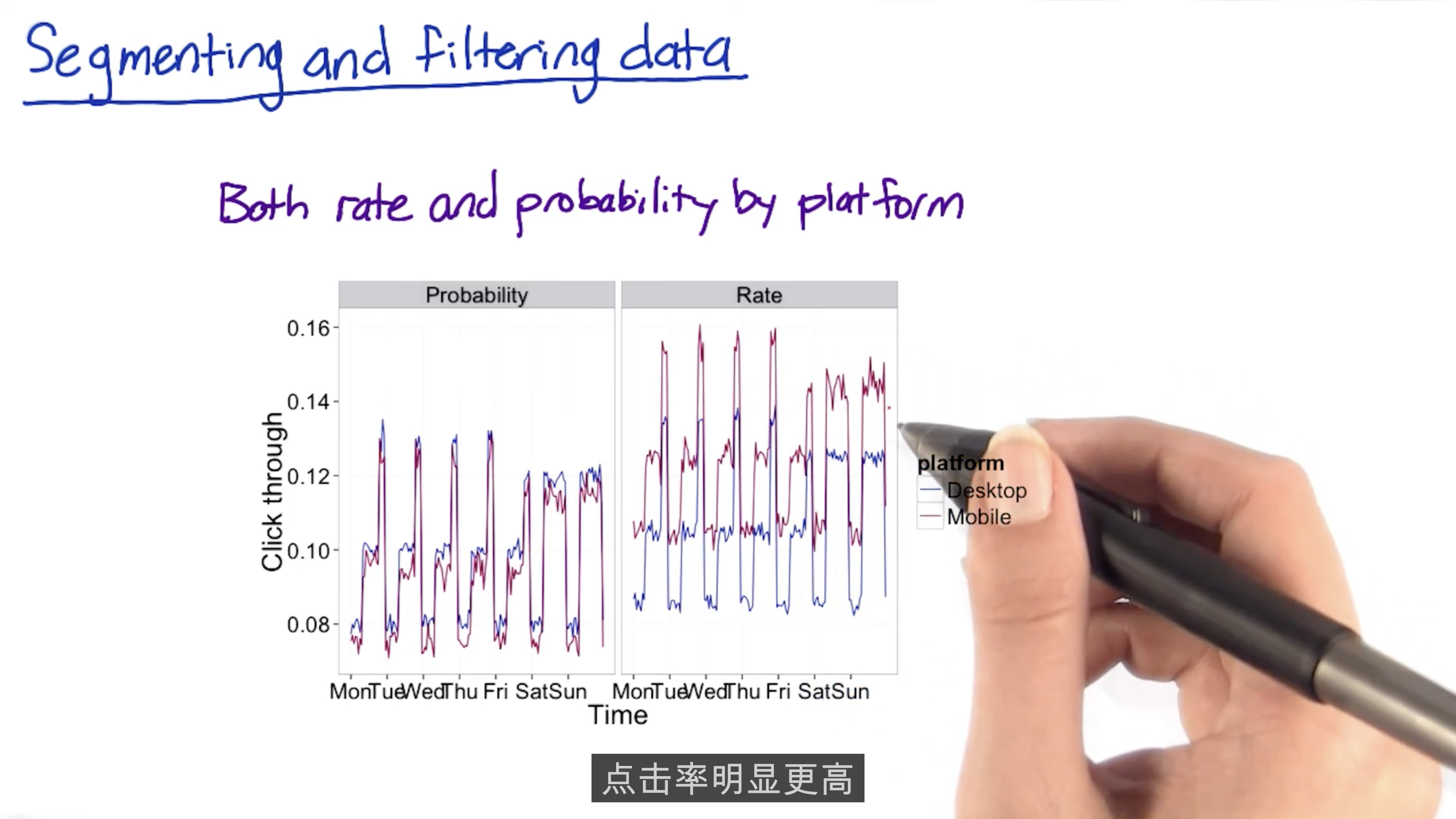
Filtering and Segmenting
The goal of filtering is to de-bias the data. But over-filtering will weaken your experiment.
Slice your data and compute your metric, such as country, language.
Summary Metrics
Sometimes, the summarization is a part of the metric definition.
Common distributions in online data
Let’s talk about some common distributions that come up when you look at real user data.
For example, let’s measure the rate at which users click on a result on our search page, analogously, we could measure the average staytime on the results page before traveling to a result. In this case, you’d probably see what we call a Poisson distribution, or that the stay times would be exponentially distributed.
Another common distribution of user data is a “power-law,” Zipfian or Pareto distribution. That basically means that the probability of a more extreme value, z, decreases like 1/z (or 1/z^exponent). This distribution also comes up in other rare events such as the frequency of words in a text (the most common word is really really common compared to the next word on the list). These types of heavy-tailed distributions are common in internet data.
Finally, you may have data that is a composition of different distributions - latency often has this characteristic because users on fast internet connection form one group and users on dial-up or cell phone networks form another. Even on mobile phones you may have differences between carriers, or newer cell phones vs. older text-based displays. This forms what is called a mixture distribution that can be hard to detect or characterize well.
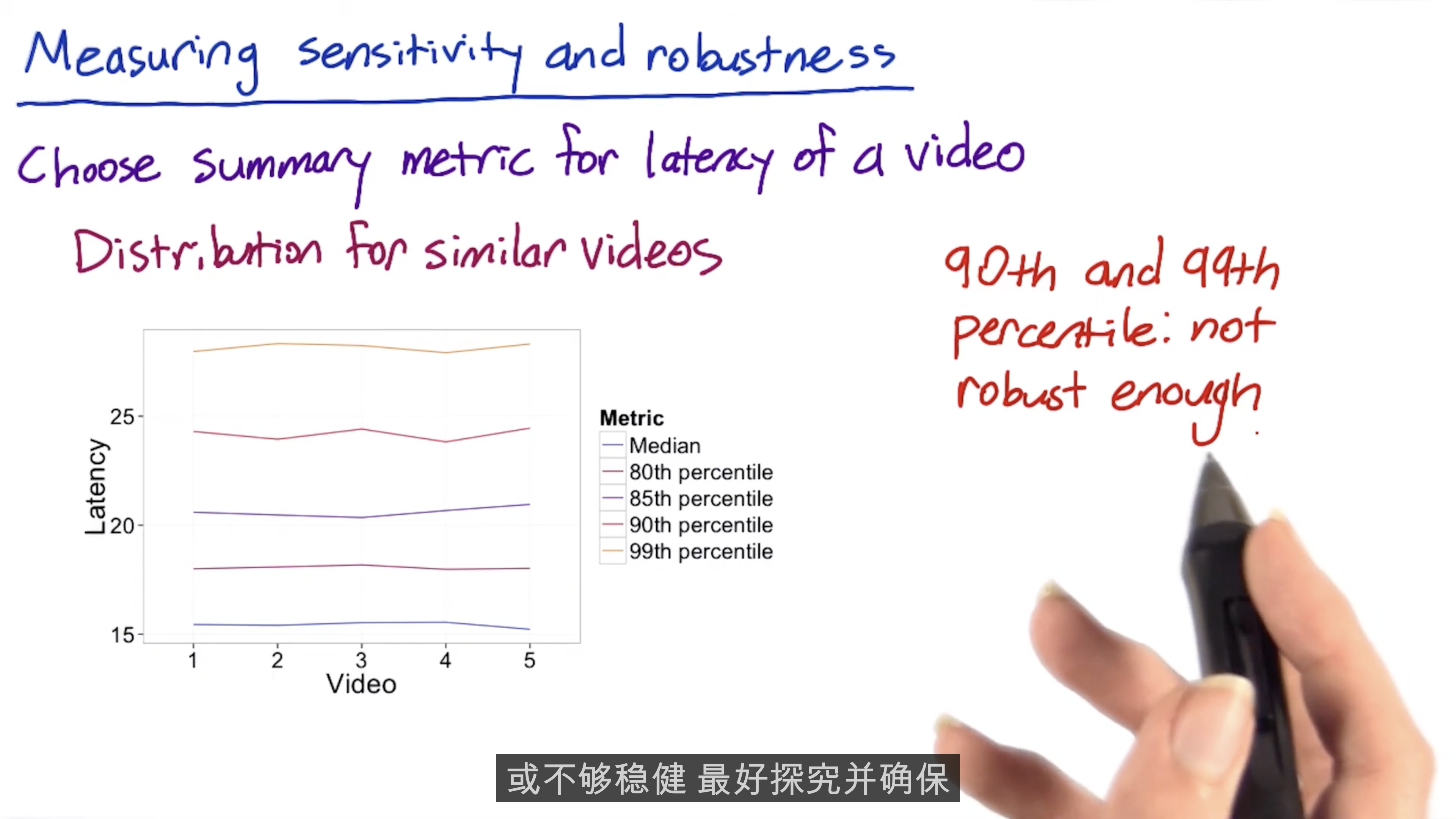
The key here is not to necessarily come up with a distribution to match if the answer isn’t clear - that can be helpful - but to choose summary statistics that make the most sense for what you do have. If you have a distribution that is lopsided with a very long tail, choosing the mean probably doesn’t work for you very well - and in the case of something like the Pareto, the mean may be infinite!
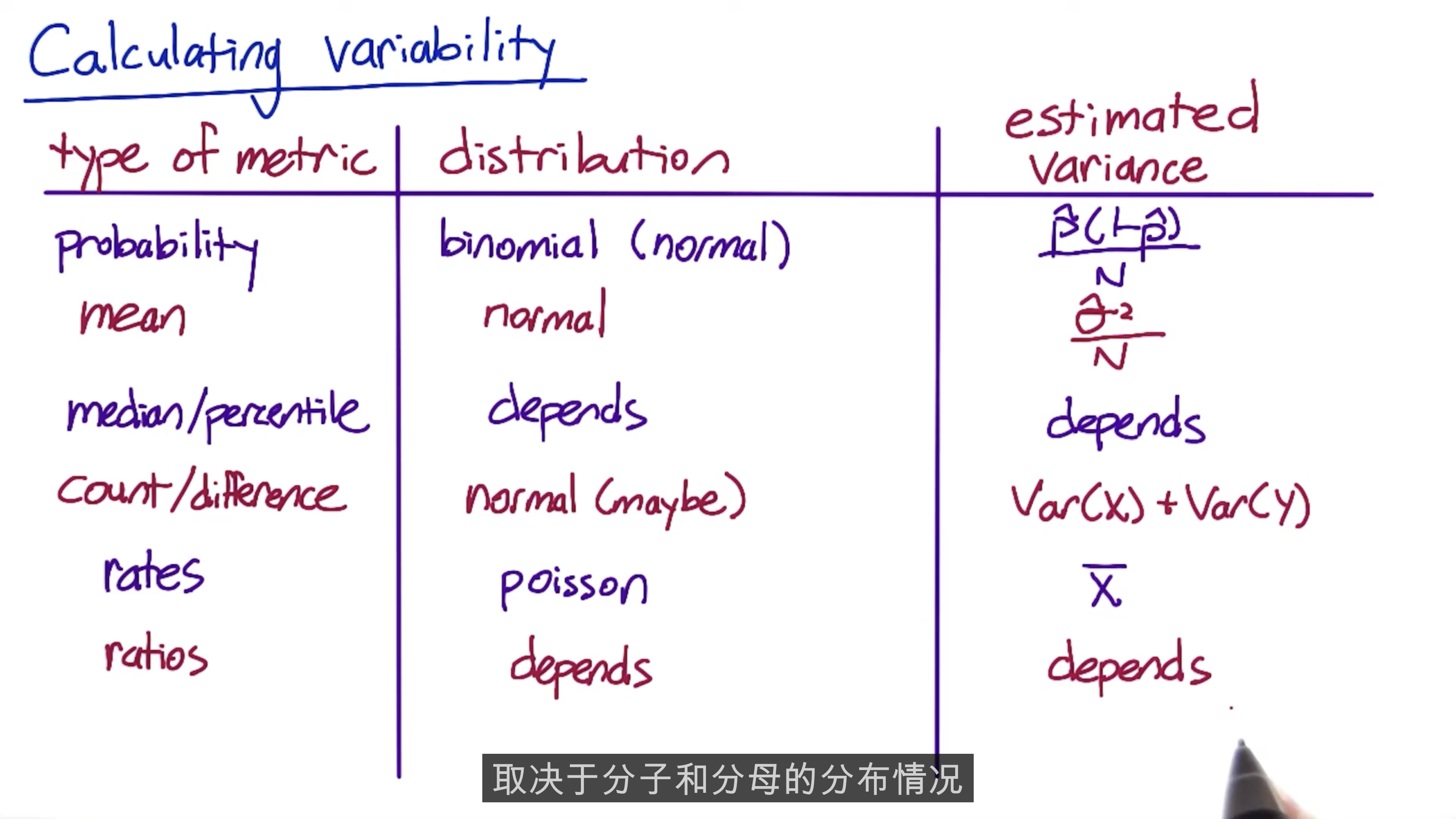
- Sum and counts
- e.g. users who visited page
- means, medians, percentiles
- e.g. mean age of users who completed a course
- e.g median latency of page load
- probabilities and rates
- Probability has 0 or 1 outcome in each case
- Rate has 0 or more
- ratios
- e.g P(revenue-generating click)/P(any click)
Why probabilities and rates are averages
To see how probabilities are really averages, consider what the probability of a single user would look like - either 1 / 1 if they click, or 0/1 if they don’t. Then the probability of all users is the average of these individual probabilities. For example, if you have 5 users, and 3 of them click, the overall probability is (0/1 + 0/1 + 1/1 + 1/1 + 1/1) divided by 5. This is the same as dividing the total number of users who clicked by the number of users, but makes it more clear that the probability is an average.
A rate is the same, except that the numerator for each pageview can be 0 or more, rather than just 0 or 1.
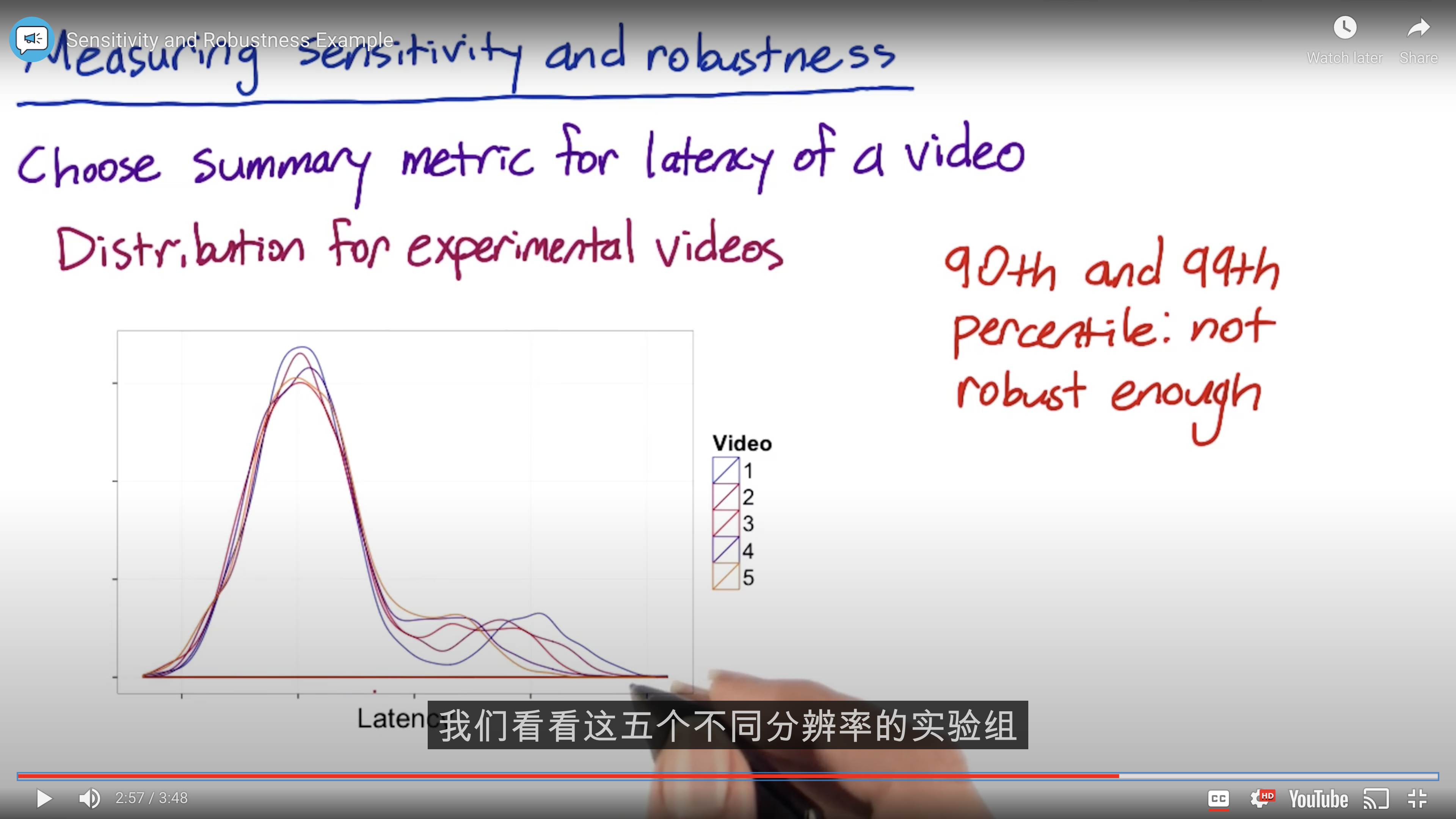
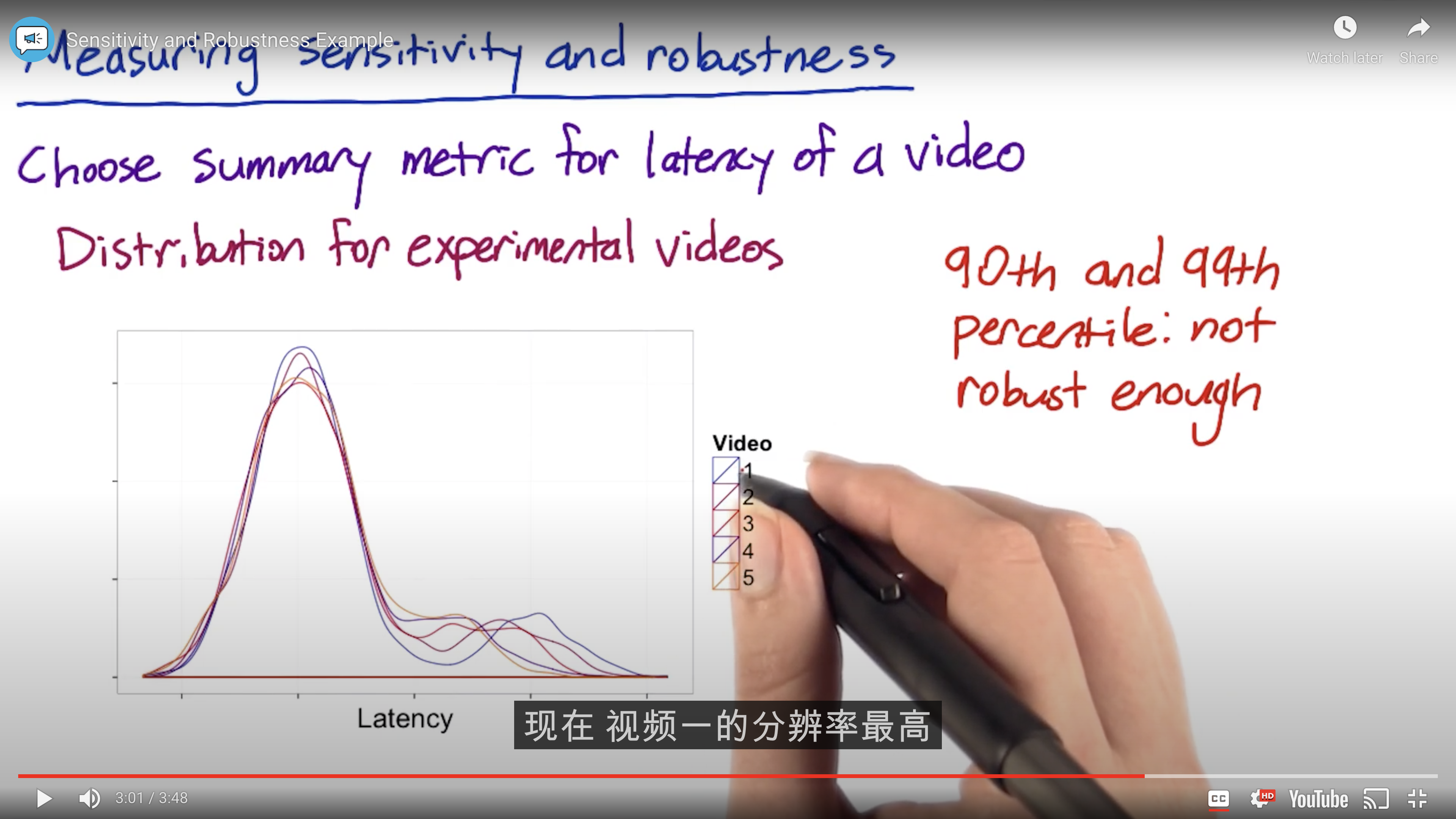
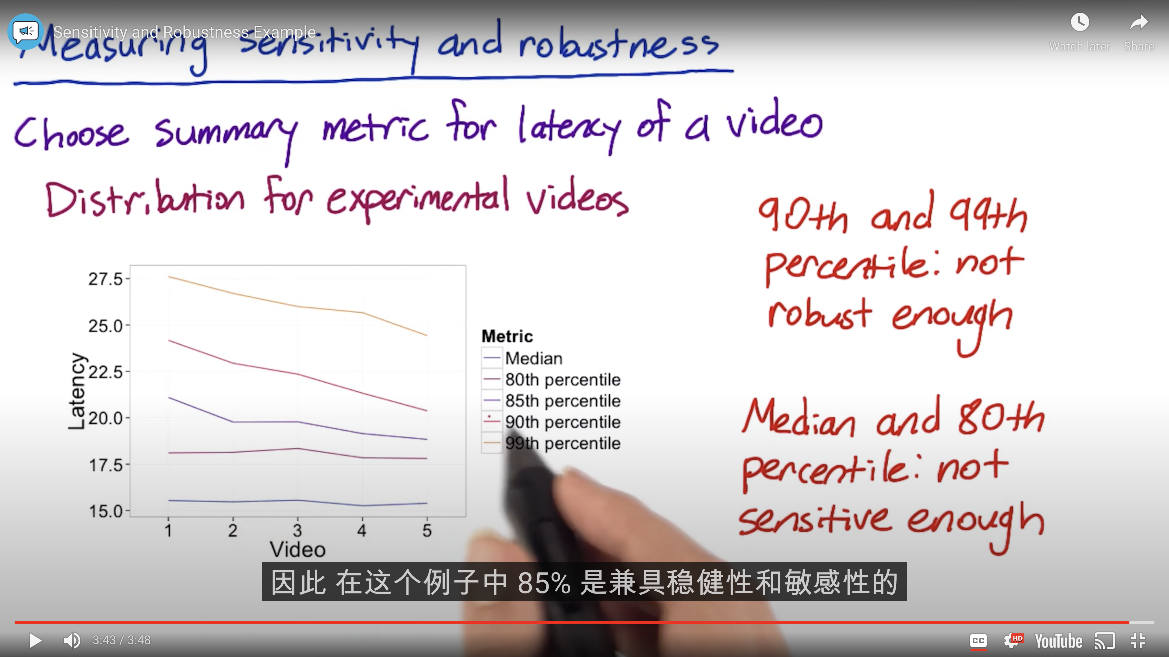
Sensitivity and Robustness
Mean may weakened by outlier.
Absolute or Relative Difference?
The main advantage of computing the percent change is that you only have to choose one practical significance boundary, to get stability over time.
One of the reason is about seasonality, and as your system is changing over time.
If you have the same practical significant boundary across the time, you can basically have the same comparison.
Absolute vs. relative difference
Suppose you run an experiment where you measure the number of visits to your homepage, and you measure 5000 visits in the control and 7000 in the experiment. Then the absolute difference is the result of subtracting one from the other, that is, 2000. The relative difference is the absolute difference divided by the control metric, that is, 40%.
Relative differences in probabilities
For probability metrics, people often use percentage points to refer to absolute differences and percentages to refer to relative differences. For example, if your control click-through-probability were 5%, and your experiment click-through-probability were 7%, the absolute difference would be 2 percentage points, and the relative difference would be 40 percent. However, sometimes people will refer to the absolute difference as a 2 percent change, so if someone gives you a percentage, it’s important to clarify whether they mean a relative or absolute difference!
Variability
Use variability to look at sizing the experiment, and analyze the confidence intervals and draw conclusions.
A metric may work under a normal circumstances but not work for us in practice, because the practical significance level may not be feasible with this metric.
Difference between Poisson variables
The difference in two Poisson means is not described by a simple distribution the way the difference in two Binomial probabilities is. If your sample size becomes very large, and your rate is not infinitesimally small, sometimes you can use a Normal confidence interval by the law of large numbers. But usually you have to do something a little more complex. For some options, see here (for a simple summary), here section 9.5 (for a full summary) and here (for one free online calculation). If you have access to some statistical software such as R (free distribution), this is a good time to use it because most programs will have an implementation of these tests you can use.
If you aren’t confident in the Poisson assumption, or if you just want something more practical - and frankly, more common in engineering, see the Empirical Variability section of this lesson, which starts here.
Quiz data
Here is the quiz data for you to copy and paste: [87029, 113407, 84843, 104994, 99327, 92052, 60684]
If you prefer, you can also make a copy of this spreadsheet. To do this, sign into Google Drive, then click “File > Make a Copy” on the spreadsheet.
Nonparametric Answers
It means you can analyze the data without making an assumption about what the distribution is.
Now, these methods can be noisier, and they can be more computationally
Example:
sign test
20 days for an experiment.
In the first 15 days, the B group has probability higher than A group in every day. Then you can use binomial to calculate the probability.
The defect is you can not draw a conclusion of effect.
The upside is, it’s pretty easy to do, and you can do it under a lot of different circumstances.
Empirical Variability
For a simple metric, you should make an assumption about the underlying distribution.
For a complex metric, the distribution may be very wired. That’s why you should shift to empirical variability.
So we use A/A experiments across the board to estimate the empirical variability of all of our metrics.
A/A test, actually no change what the users seen, may cause difference due to the underlying variability such as your system of the user population, what users are doing, all of those types of things.
For example, if you see a lot of variability in a metric in an A/A test, it’s probably too sensitive to be useful in evaluating a real experiment.
Google will use ten, twenty, or several hundreds of A/A test to prove the sensitivity and robustness.
Clearly there’s a diminishing return as you run more A/A test.
The key rule of them is keep in mind is that the standard deviation is going to be proportional to the square root of the number of sample.
One method is to run a big experiment and bootstrap it.
A/A test data
Uses of A/A tests:
- Compare results to what you expect (sanity check)
- Estimate variance and calculate confidence
- Directly estimate confidence interval
This spreadsheet contains the data, calculations, and graphs shown in the video.
If you want to make any changes to it, you’ll need to sign into Google Drive, then copy it using “File > Make a Copy”.
A/A test data
You can find the data for the quiz in this spreadsheet.
Use empirical standard deviation instead of the analytic standard error for calculating margin of error.
If you want to make changes to it, you’ll need to sign into Google Drive, then copy it using “File > Make a Copy”.
For empirical CI, just bootstrap the sample data, and take the left 2.5% data and right 2.5% as the CI left boundary and right boundary.
Variability Summary
- Different metric has different variability
- So some variabilities may so high for a metric use, not practical to use in a experiment, even if the metric makes a lot of business or product sense.
Some metrics may too stable to meaningful, such as task per user per day (search).
So, understand your data, understand your system, and incorporate with your engineer team to know how data is captured.
Run analytical characterization first, it may comes up enough result or help you to size your experiment. You have to look at the distribution and start to get feel of the data.
Designing an Experiment
- Choose subject
- Choose population
- Size
- Duration
Unit of Diversion
How to assign the content to A and B groups?
What if the user refresh the page and see the change?
So usually for the visible change, you need to assign it based on people instead of event.
Unit of Diversion: how we define what an individual subject is in the experiment
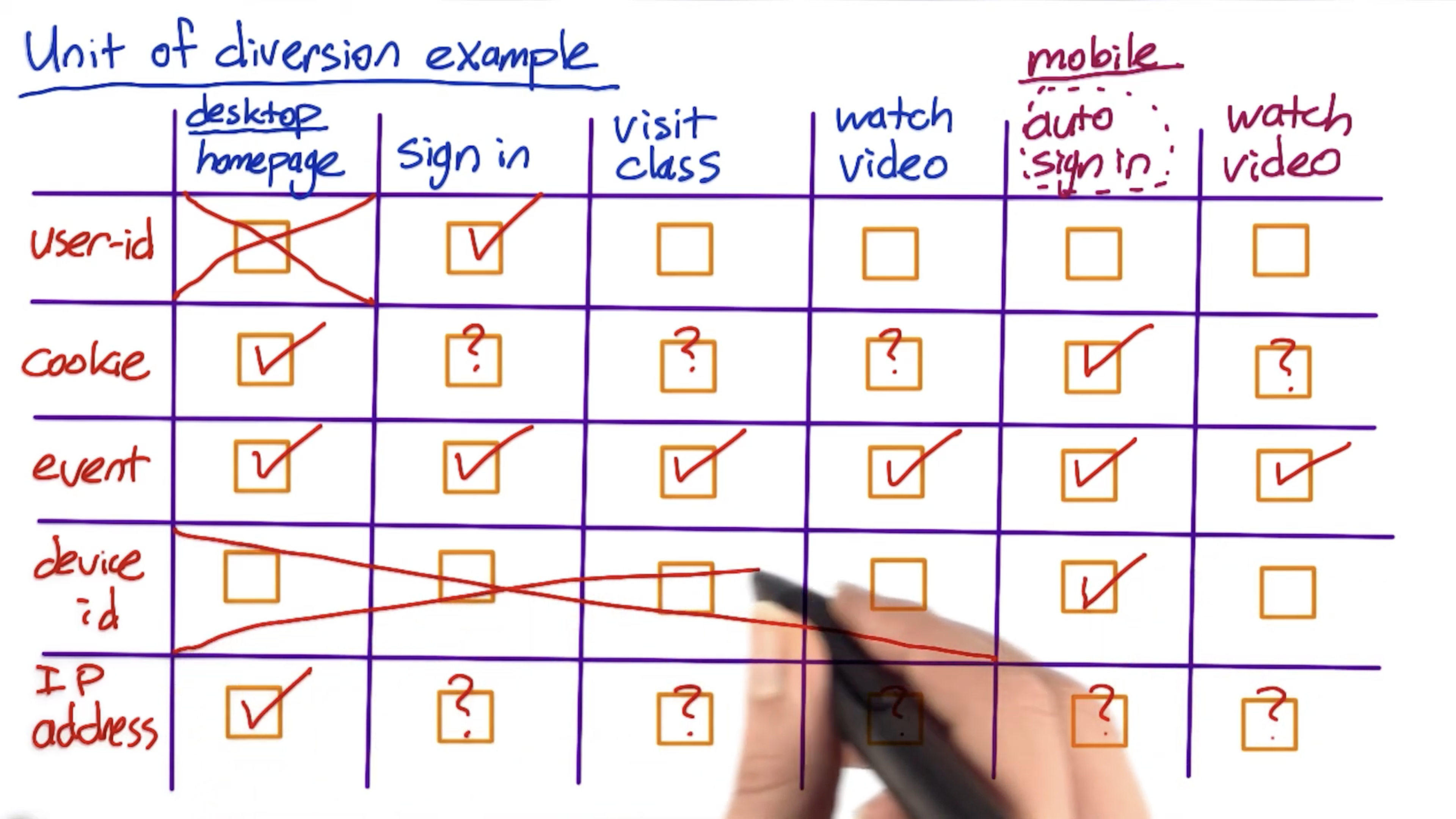
The following are some units of diversion:
- User ID
- Stable, unchanging
- Personally identifiable
- Anonymous id (cookie)
- Changes when you switch browser or device
- Users can clear cookies
- Event
- No consistent experience
- Use only for non-user-visible changes
Less common:
- Device id
- only available for mobile
- tied to specific device
- unchangeable by user
- personally identifiable
- IP address
- changes when location changes
Consistency of Diversion
User consistency: For logged users, even if they change the device, the user’s experience is consistent.
For maintaining the consistent user’s experience and collect immutable user data, we should provide minimum and enough consistency.
For example, if we wonder wether the button color will user’s behavior or not, we cannot provide different color for the same user. If we do so, we may collect two different choices from the same user.
Consistency of Diversion(from high to low)
- User ID
- Add Instructor’s notes before quizzes
- Users will almost certainly notice
- Cross-device consistency important
- Add Instructor’s notes before quizzes
- Cookie
- Change button color and size
- Distracting if button changes on reload
- Different look on different devices is OK. Because the UI in different devices are usually different.
- Change button color and size
- Event
- Change reducing video load time
- Users probably won’t notice
- Change order of search results
- Users probably won’t notice
- Change reducing video load time
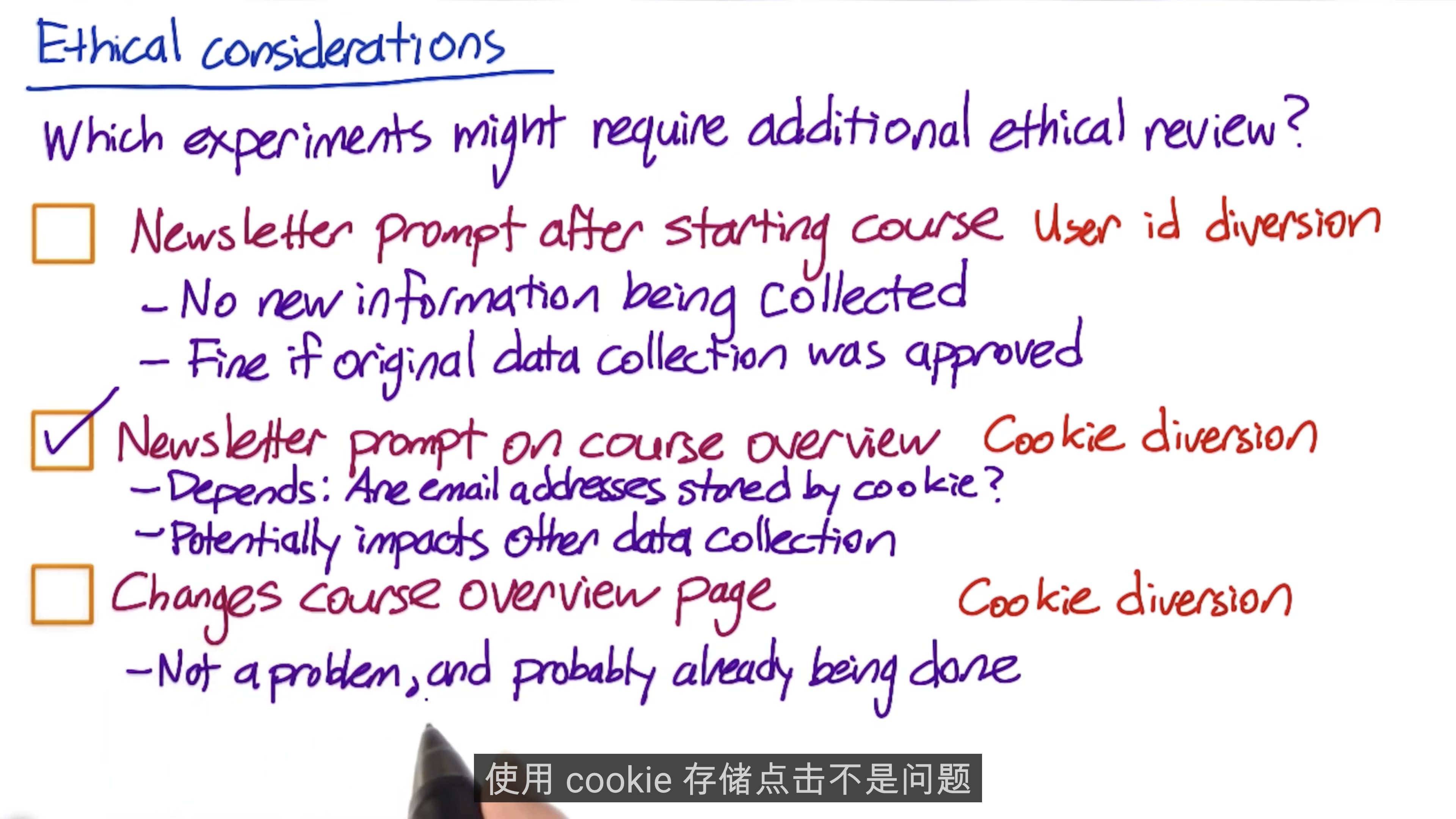
Ethical Considerations for Diversions
If you gather data by user id, the data is identifiable.
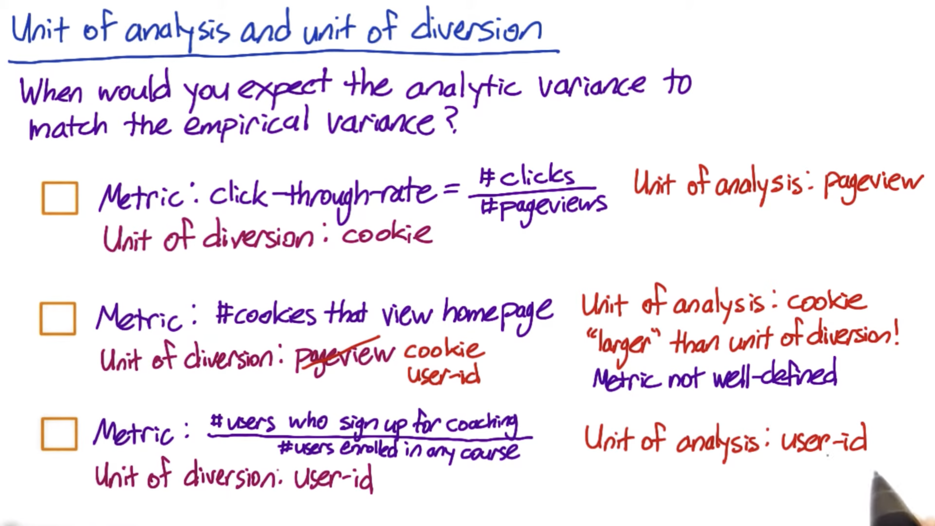
Unit of Analysis vs. Unit of Diversion
Changing the unit of diversion can change the variability of metric, sometimes pretty dramatically.
When unit of analysis = unit of diversion, variability tends to be lower and closer to analytical estimate.
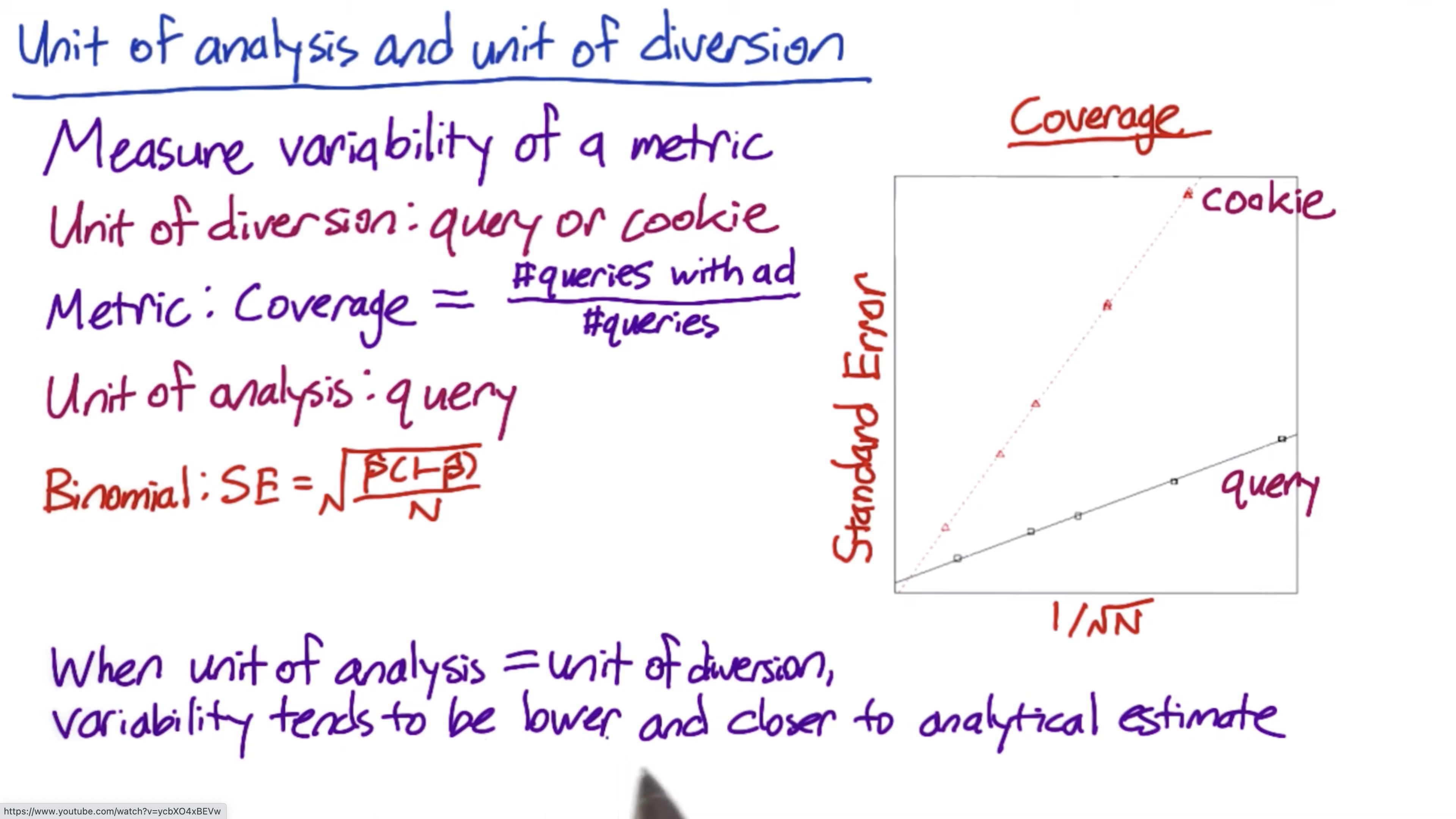
Standard error graph
The graph Caroline discusses is Figure 4 in the following paper.
Inter- vs. Intra-User Experiment
Interleaved experiments
In an interleaved ranking experiment, suppose you have two ranking algorithms, X and Y. Algorithm X would show results X1, X2, … XN in that order, and algorithm Y would show Y1, Y2, … YN. An interleaved experiment would show some interleaving of those results, for example, X1, Y1, X2, Y2, … with duplicate results removed. One way to measure this would be by comparing the click-through-rate or -probability of the results from the two algorithms. For more detail, see this paper.
Targe Population
You need to define the population based on your users’ backgrounds, such as the users’ location, time of using you website.
If you mix population and sample data, you may get much lower result, in comparison to only control and treatment groups.
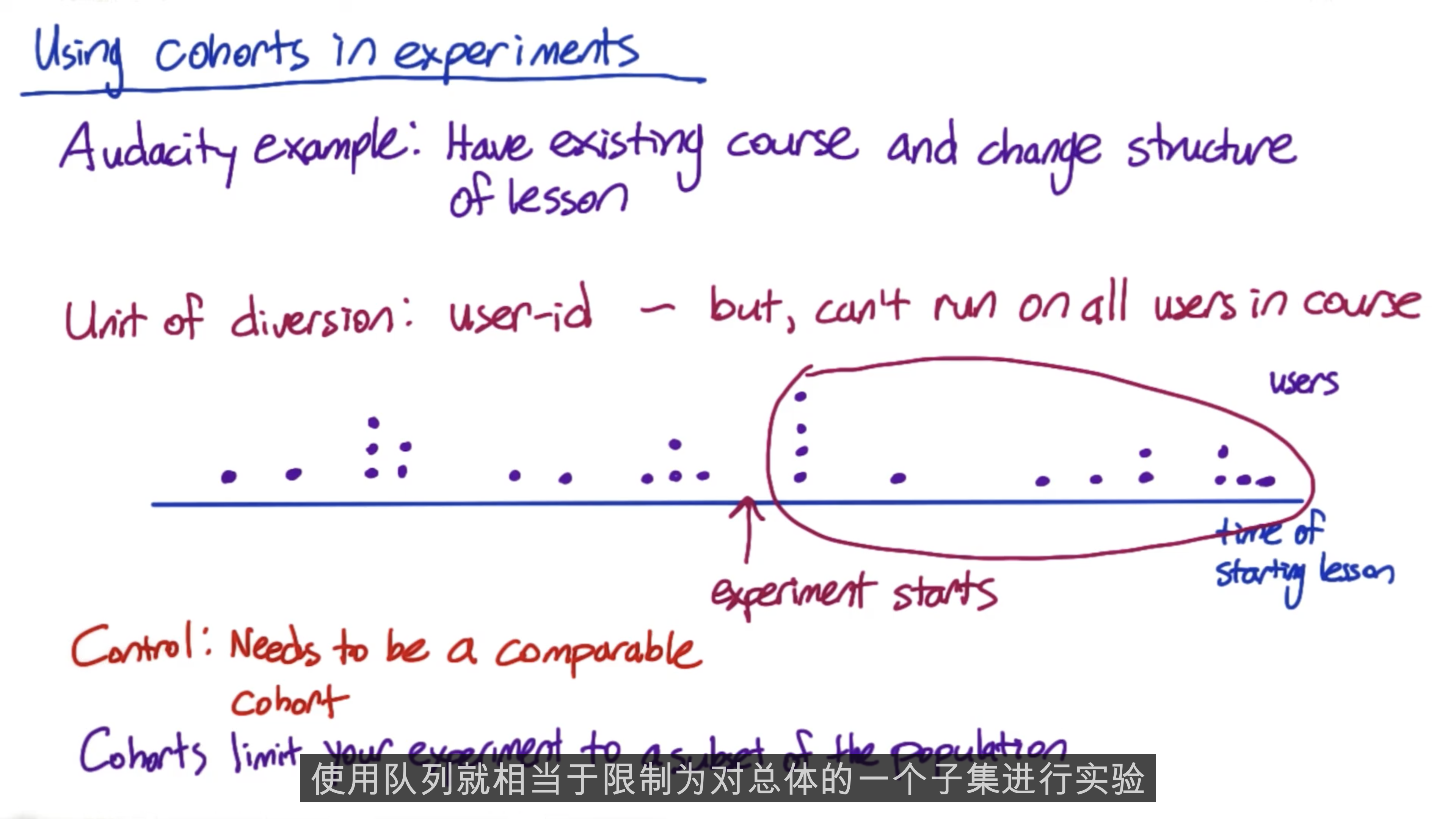
Population vs. Cohort
Cohort is hard to analyze, and they’re going to take more data because you’ll lose users. So typically, you only want to use them when you’re looking for yser stability. So say, you have a learning effect or you want to measure something like increasing usage of the site or increased usage of a mobile device.
Experiment Design and Sizing
The key thing to keep in mind is that this is an iterative process, which means you may need to try different combination of unit diversion, population, and etc.
Sizing: Example
https://classroom.udacity.com/courses/ud257/lessons/4001558669/concepts/39700990240923
How variability affects sizing.
Audacity includes promotions fro coaching next to videos.
Experiment: Change wording of message
Metric: Click-through-rate = #clicks/#pageviews
Unit of diversion: pageview, or cookie
Analytic variability won’t change, but probably under-estimate for cookie diversion
Empirical estimate with 5,000 pageviews
- By pageview: 0.00515
- By cookie: 0.0119
To calculate size, assume $SE ~ \frac{1}{\sqrt{N}}$
Sizing calculation code
You can find the R code Caroline used to calculate the experiment size in the Downloadables section.

1 | import numpy as np |
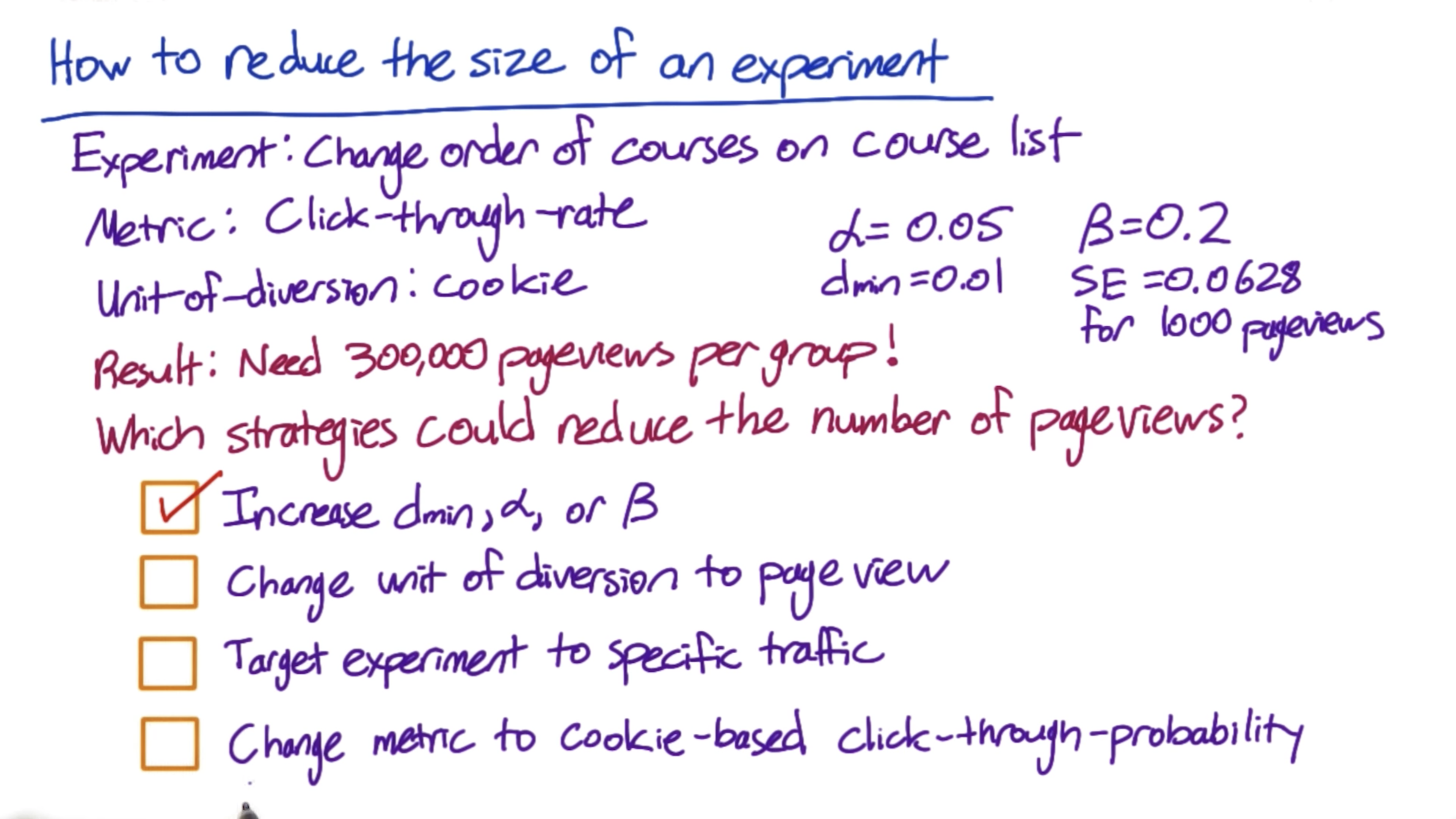
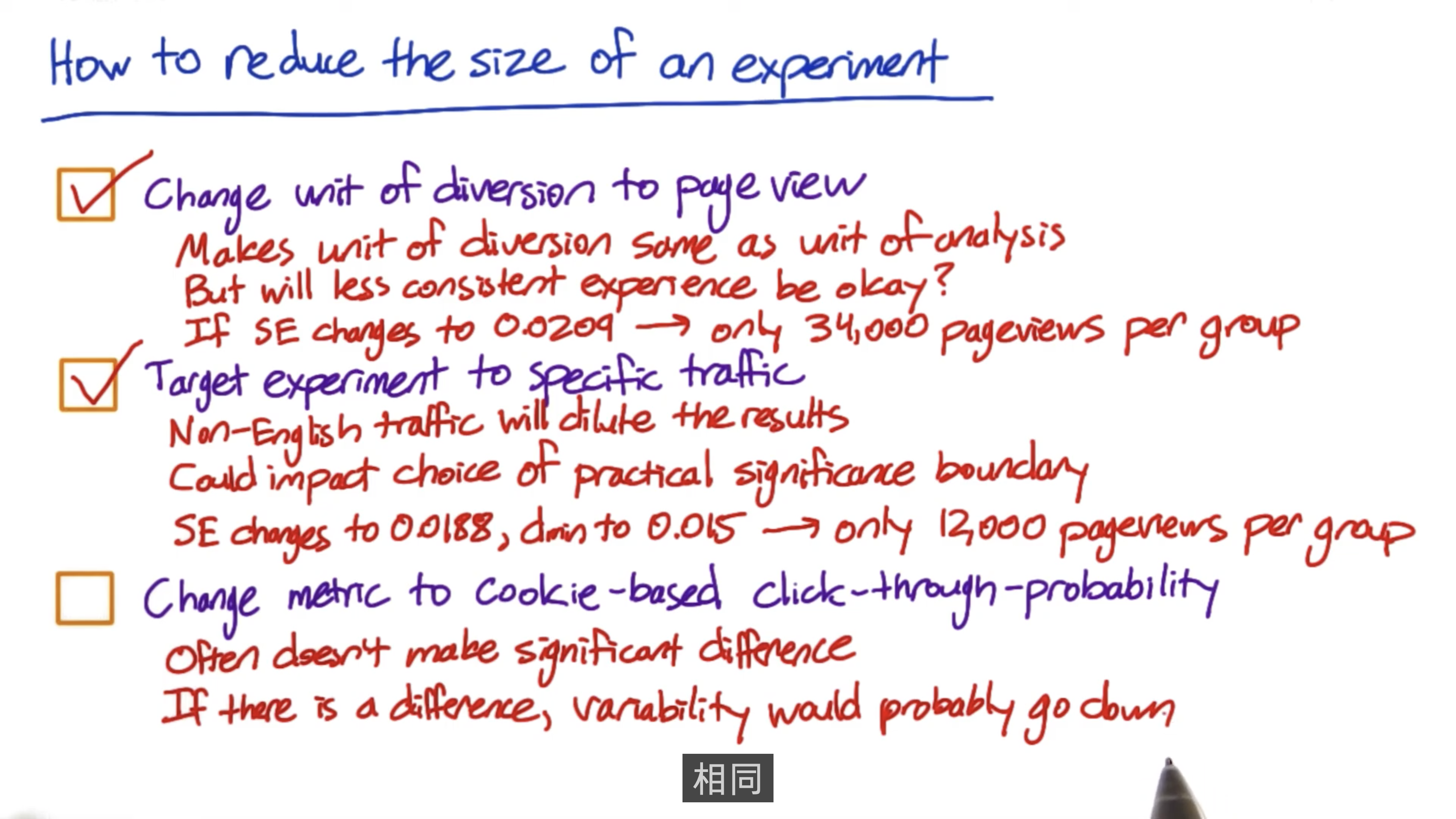
How to Decrease Experiment Size
Sizing Triggering
- It’s hard to predict the potential impact on all of the users.
- Consider how you detect the impact.
- If you really don’t know what fraction of your population is going to be affected, you’re going to have to be pretty conservative when you plan how much time and how many users have to see your experiment.
- It’s better to either run a pilot where you turn on the experiment for a little while and see who’s affected, or you can even just use the first day or the first week of data to try to get a better guess at what fraction of your population you’re really looking at.
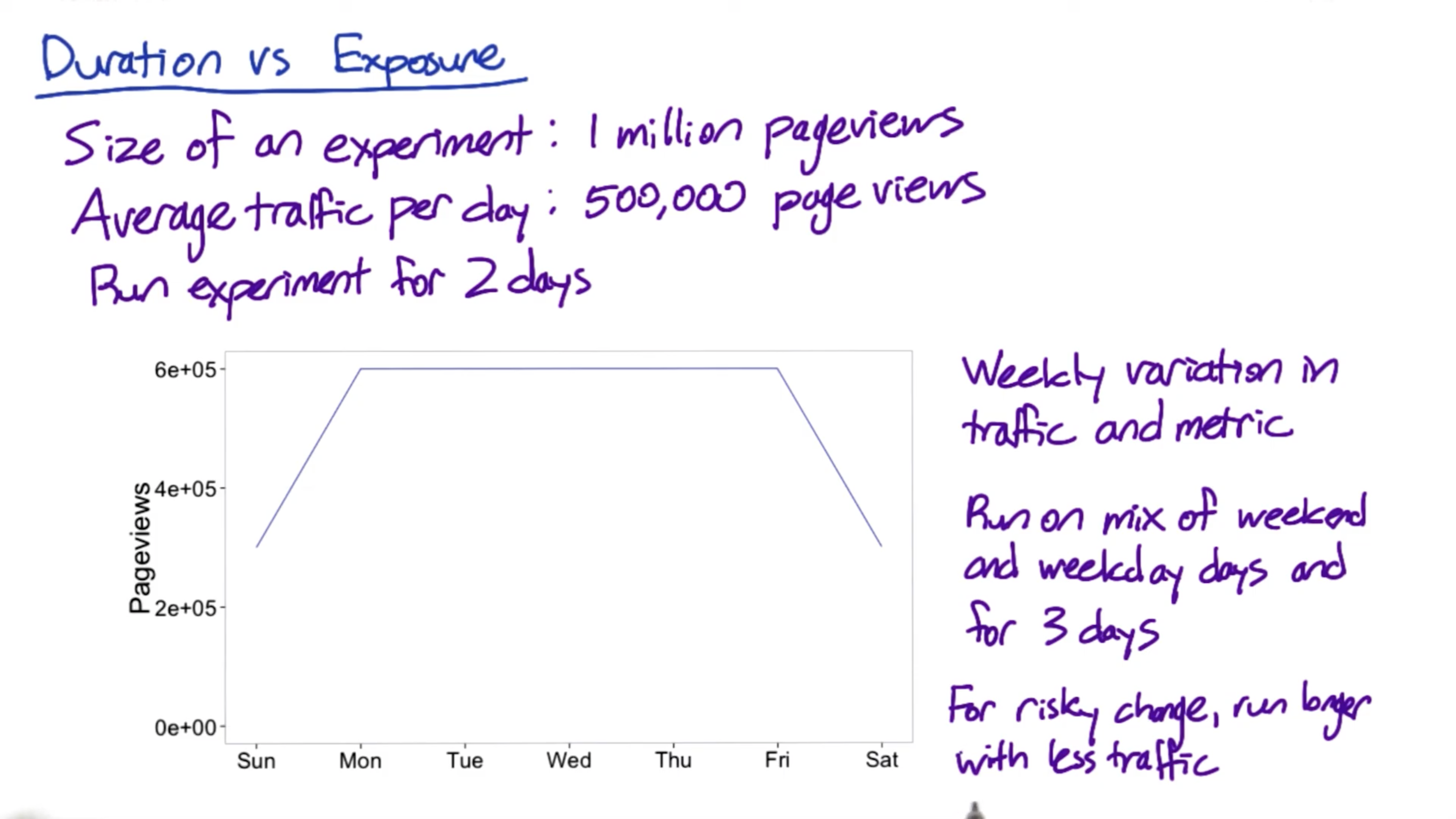
Duration vs. Exposure
- How long
- When
- What fraction of your traffic you’re going to send through the experiment.
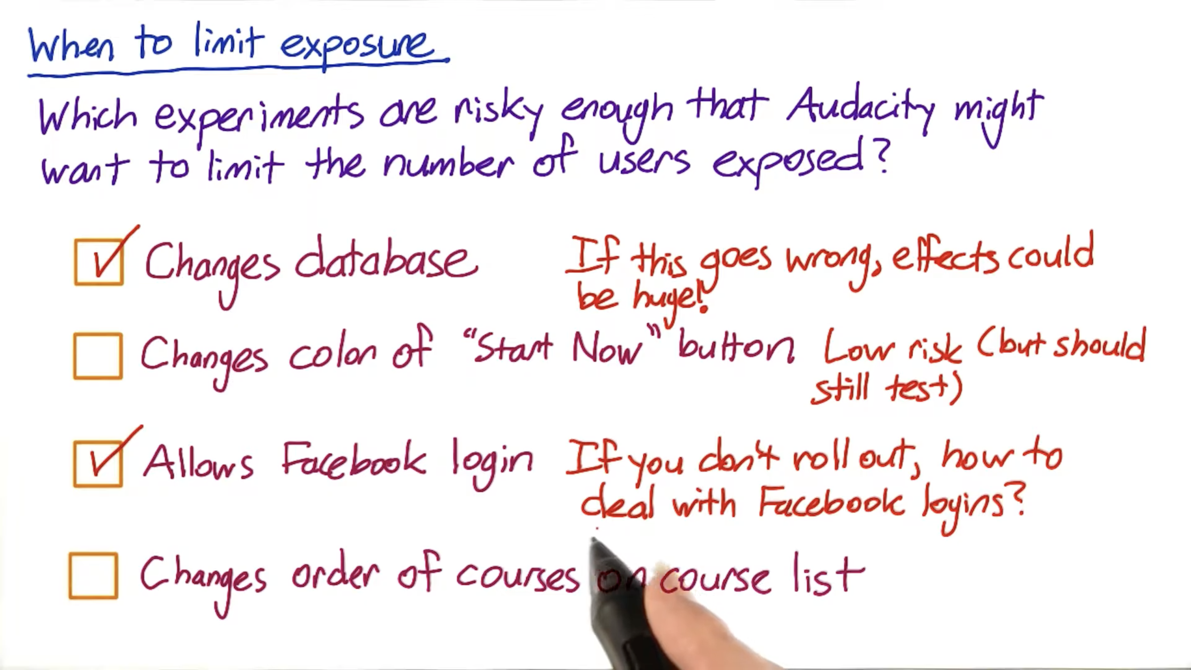
DO NOT send traffic to all of the users:
- Safety. You should keep the site mostly the same since you don’t know the impact of the new features.
- Press
- A relative too short-term experiment may bring a huge impact from some other reasons instead of your features, such as weekend, holidays, or a specific time range in a day.
And the other option is, you may be running multiple tasks at your company or you may be running multiple tasks of the same feature with different levels of a parameter or different types of the same feature? And if you really want those things to be directly comparable, the easiest thing to do is to run them at the same time on smaller percentages of traffic. And then you know that if one of the tests was affected by a holiday or a strange shift in your traffic, they all were, and you should be able to compare the relative ordering of the tests against each other.
When to Limit Exposure
Learning Effects
Learning effects is basically when you want to measure user learning. Or effectively whether a user is adapting to a change or not. The key issue with trying to measure a learning effect is time.
Dosage: how often the users can see the change.
In pre-period:
Make sure the difference is from the experiment instead of any preexisting and inherent differences in your population such as system and users’ variability. In other words, don’t forget AA test.
In post-period:
If there any differences in the experiment and the control populations after I’ve run my experiment, then I can attribute those differences to user learning that happened in the experiment period. It means your users may adapt the new feature and react with it.
Lessons Learned
Just do it.
Even failed experiments will provide a framework.
Analyzing Results
- Sanity Checks
- Single Metric
- Multiple Metrics
- Gotchas
Sanity Checks
There are all sorts of things that can go wonky that could really invalidate your results.
For example, maybe something went wrong in the experiment diversion and now your experiment and control groups aren’t comparable. Or maybe you use some filters and you set up the filter differently in the experiment and the control. Or you set up data capture and your data capture isn’t actually capturing the events that you want to look for in your experiment.
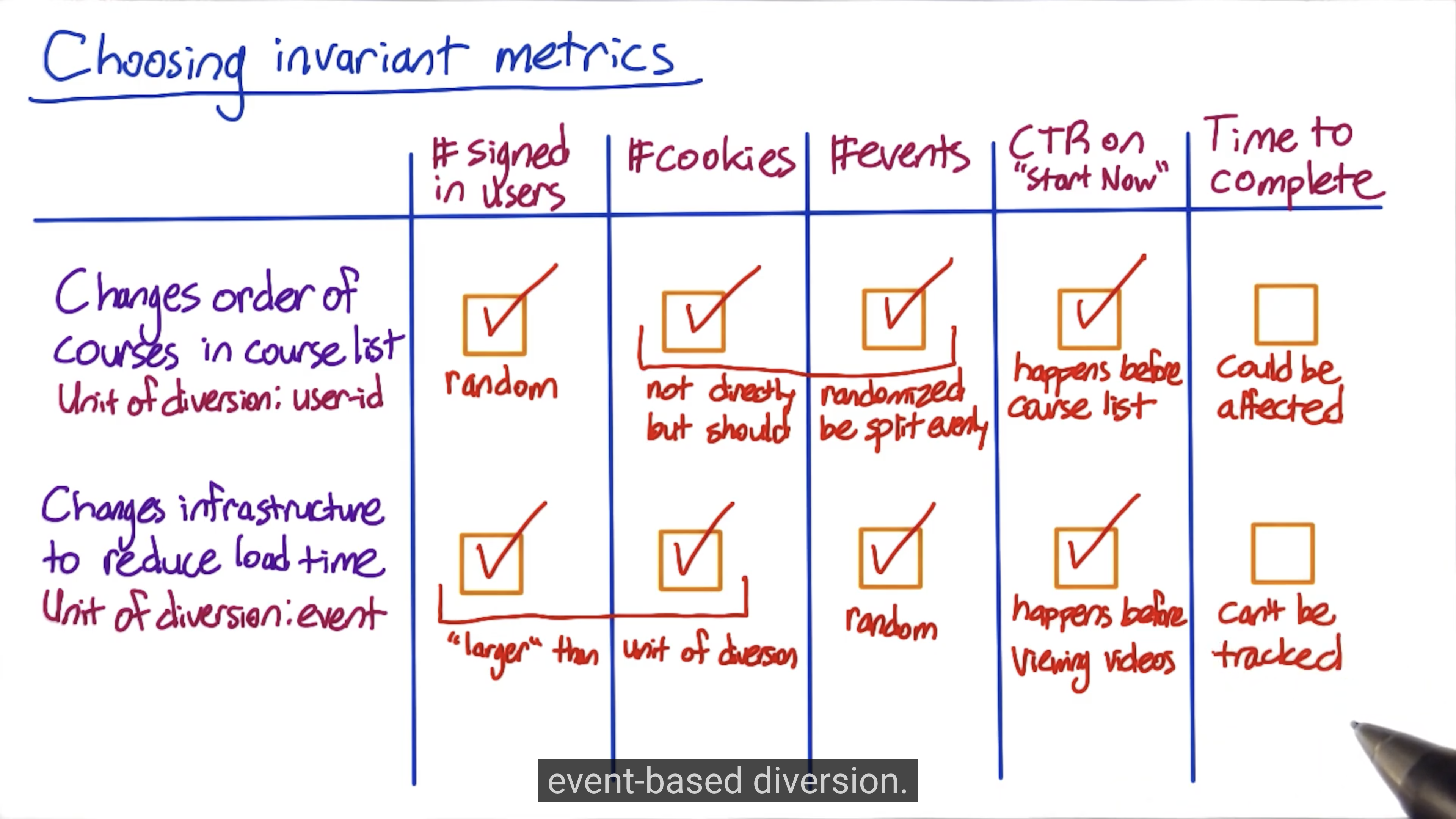
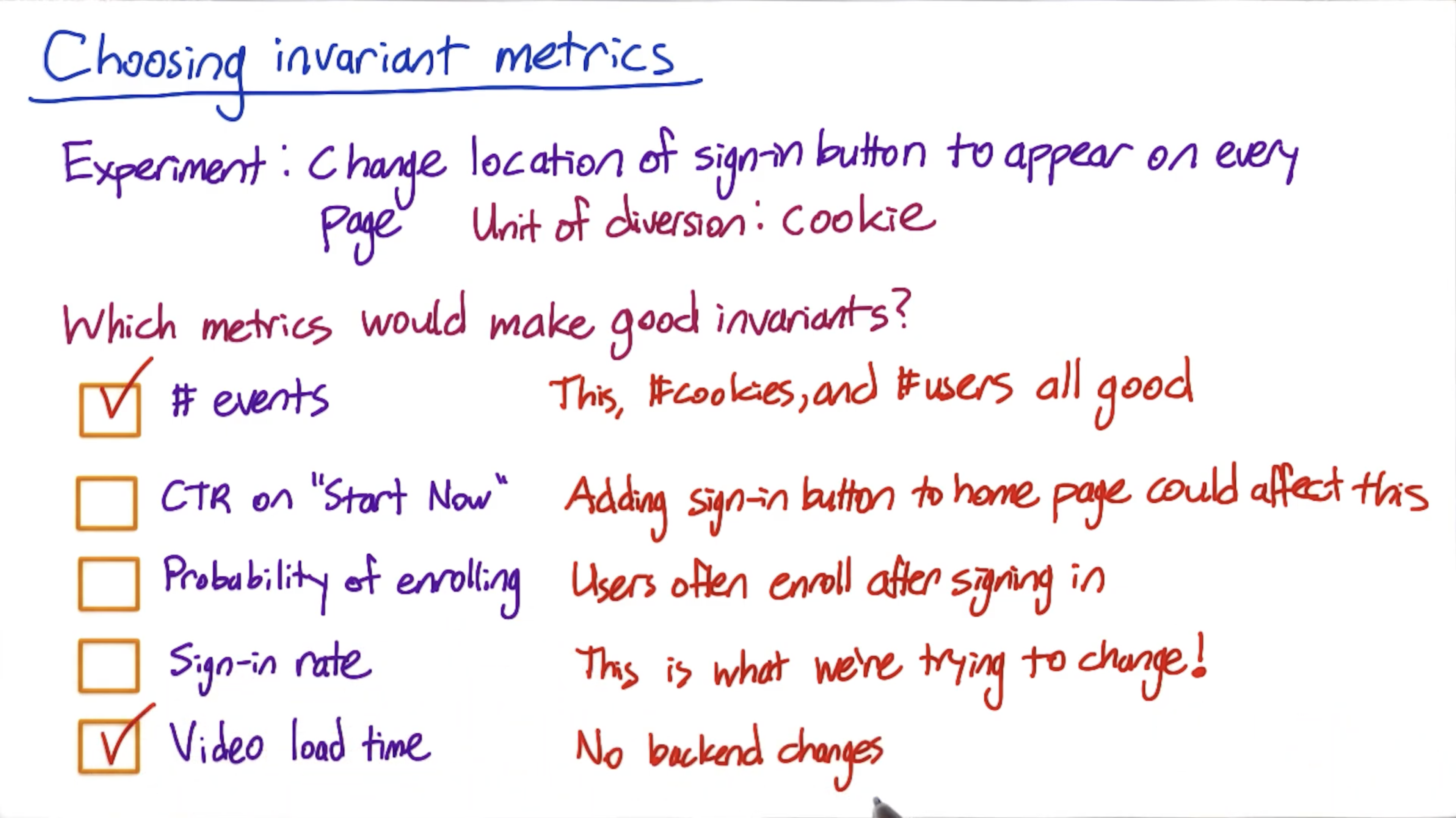
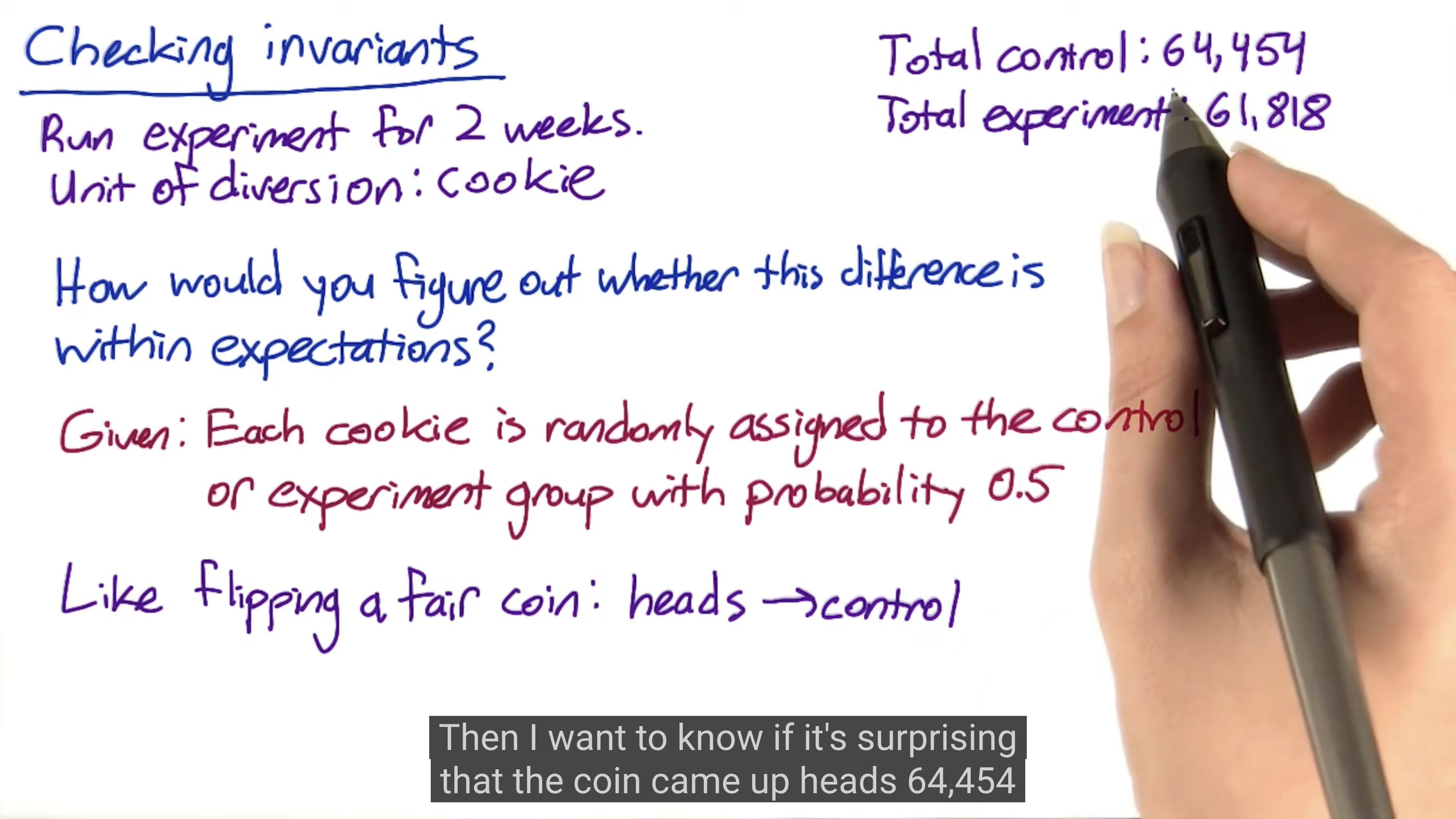
Invariant metrics:
- Population sizing metrics, based on your unit of diversion. Your population of control and experiment should be comparable.
- Actual invariants, those metrics that shouldn’t change when you run your experiment.
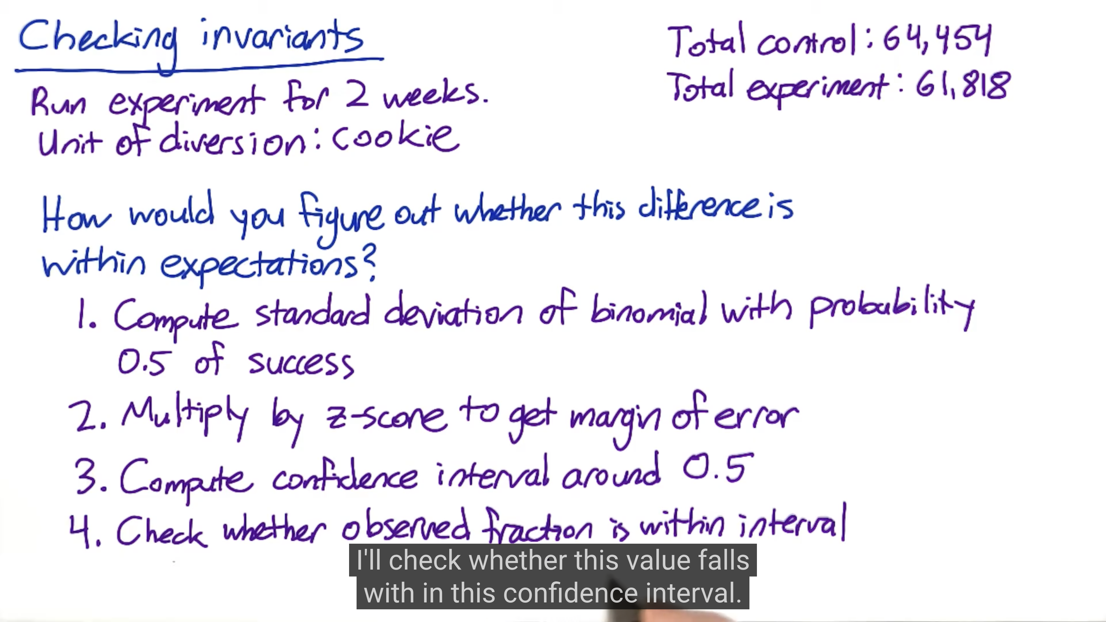
Invariant metrics are the metrics that should not change during your experiment. So you need to check if they changed in the Sanity Checks. After this step, you can try to analyze your data.
Choosing Invariants
Checking invariants
1 | import math |
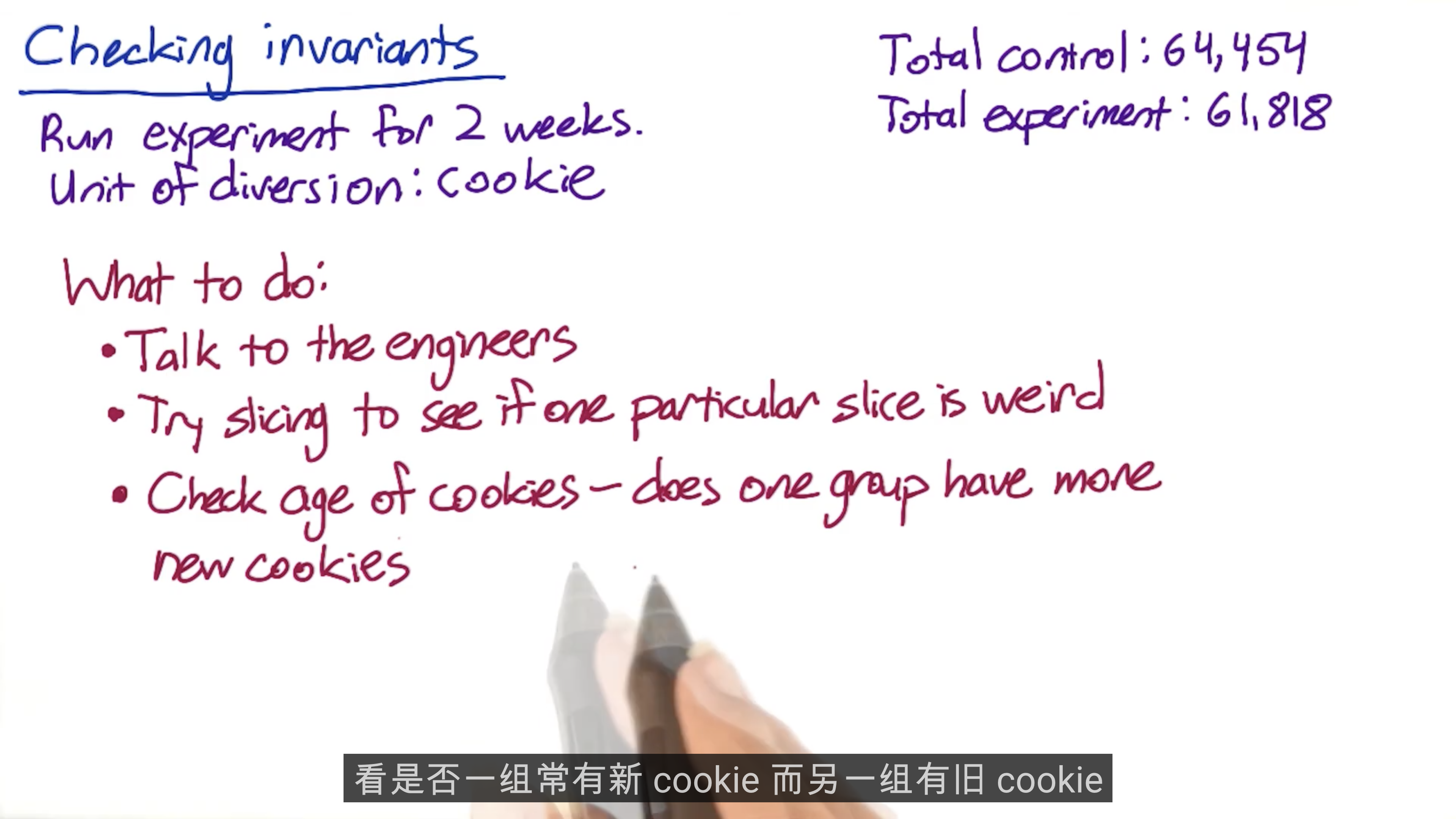
Sanity Checking: Wrapup
If your sanity check is wrong, don’t pass go.
If there is an issue, you need to check every step. Basically, the learning effect will not cause a sharp change. The change should happen over time.
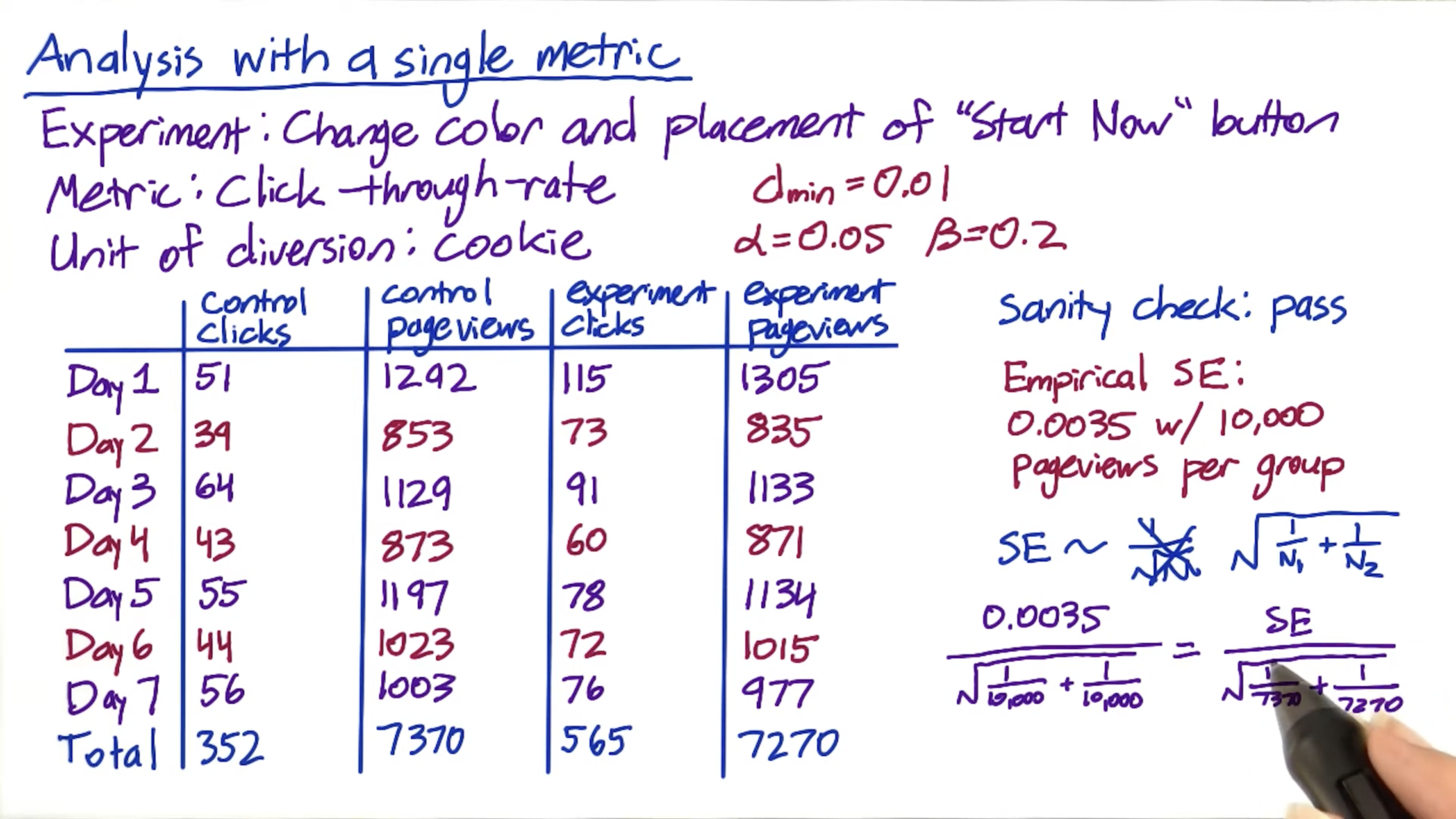
Single Metric: Introduction
The goal is to make a business decision about whether the experiment has favorable impacted your metrics.
Extend your experiment and break it down into different platforms or etc can help you debug and give you new hypothesis about how people reacting to the experiment.

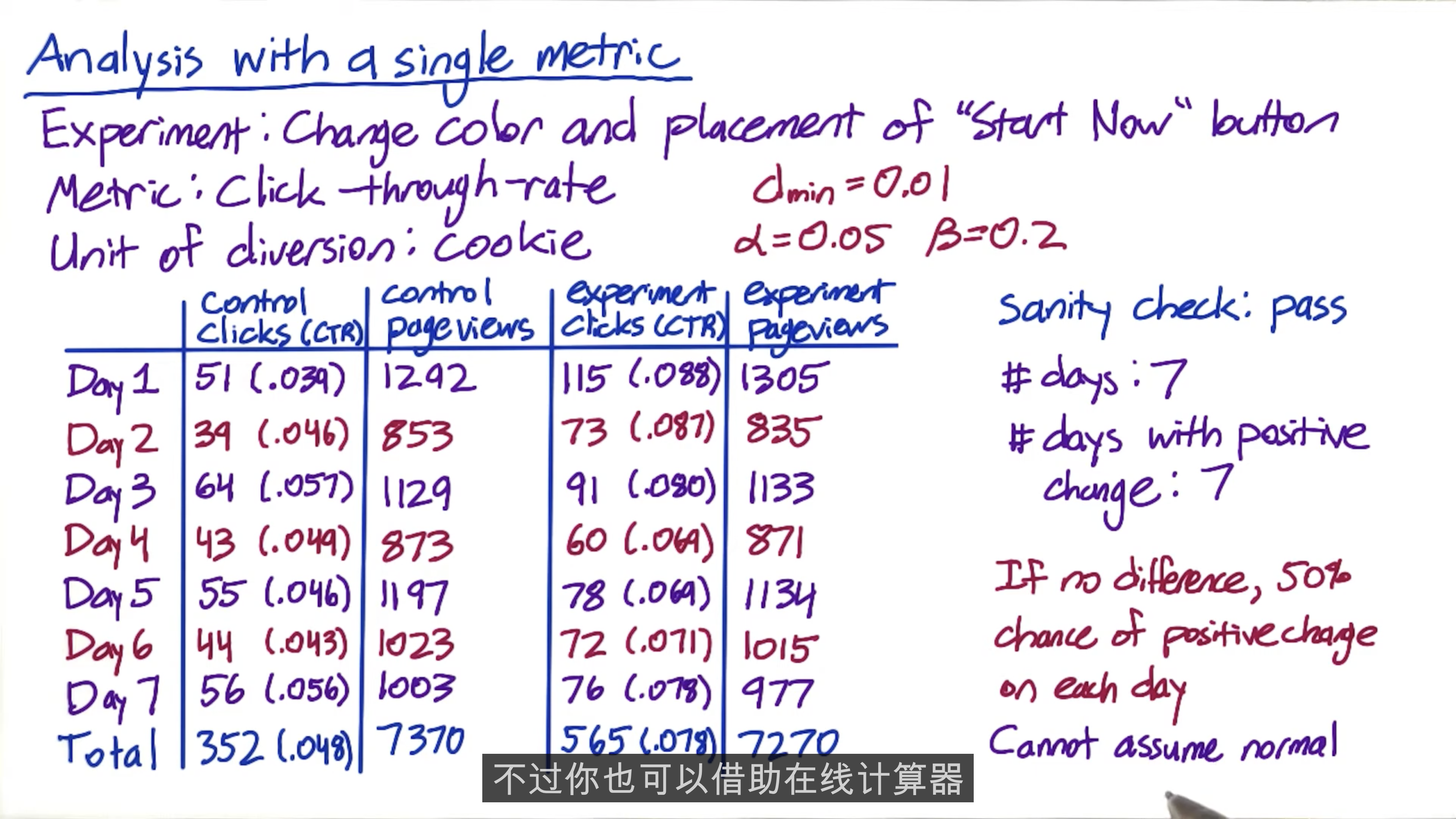
Sign test, Nonparametric
The sign test has lower power than the effect size test, which is frequently the case for nonparametric tests.
That’s the price you pay for not making any assumptions.
That is not necessarily a red flag, but it’s worth digging deeper and seeing if we can figure out what’s going on.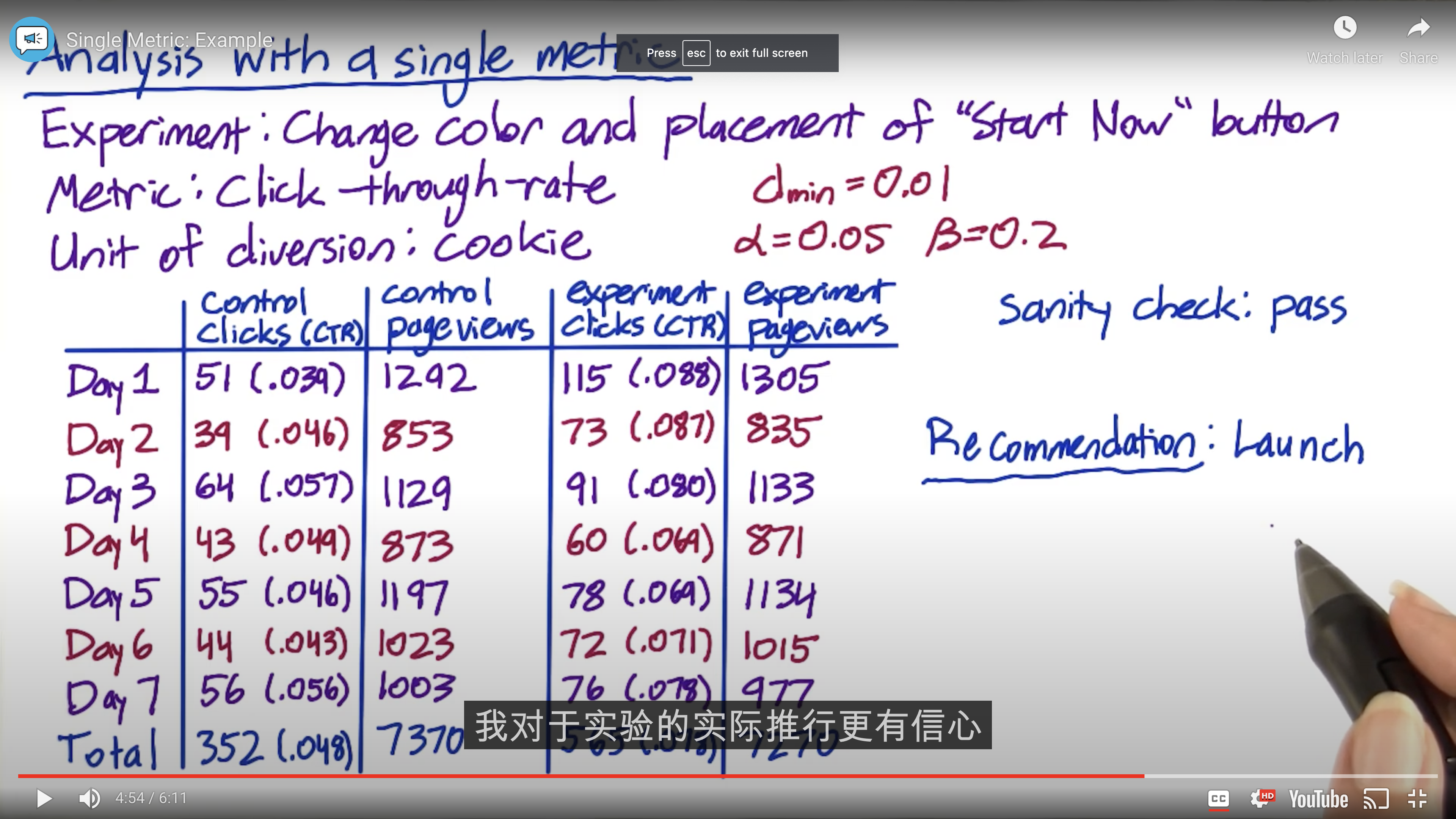
Online calculator
You can do a sign test calculation using this online calculator.
Quiz data
Here is the quiz data for you to copy and paste:
Xs_cont = [196, 200, 200, 216, 212, 185, 225, 187, 205, 211, 192, 196, 223, 192]
Ns_cont = [2029, 1991, 1951, 1985, 1973, 2021, 2041, 1980, 1951, 1988, 1977, 2019, 2035, 2007]
Xs_exp = [179, 208, 205, 175, 191, 291, 278, 216, 225, 207, 205, 200, 297, 299]
Ns_exp = [1971, 2009, 2049, 2015, 2027, 1979, 1959, 2020, 2049, 2012, 2023, 1981, 1965, 1993]
If you prefer, you can also make a copy of this spreadsheet. To do this, sign into Google Drive, then click “File > Make a Copy” on the spreadsheet.
1 | import pandas as pd |
1 | # Detexify http://detexify.kirelabs.org/classify.html |
1 | display(Latex(r"$\displaystyle MOE_{\gamma} = Z_{\gamma} \times SE$")) |
1 | # Calculate estimated difference d |
1 | # Draw conclusion |
1 | # Sign test |
Single Metric: Gotchas
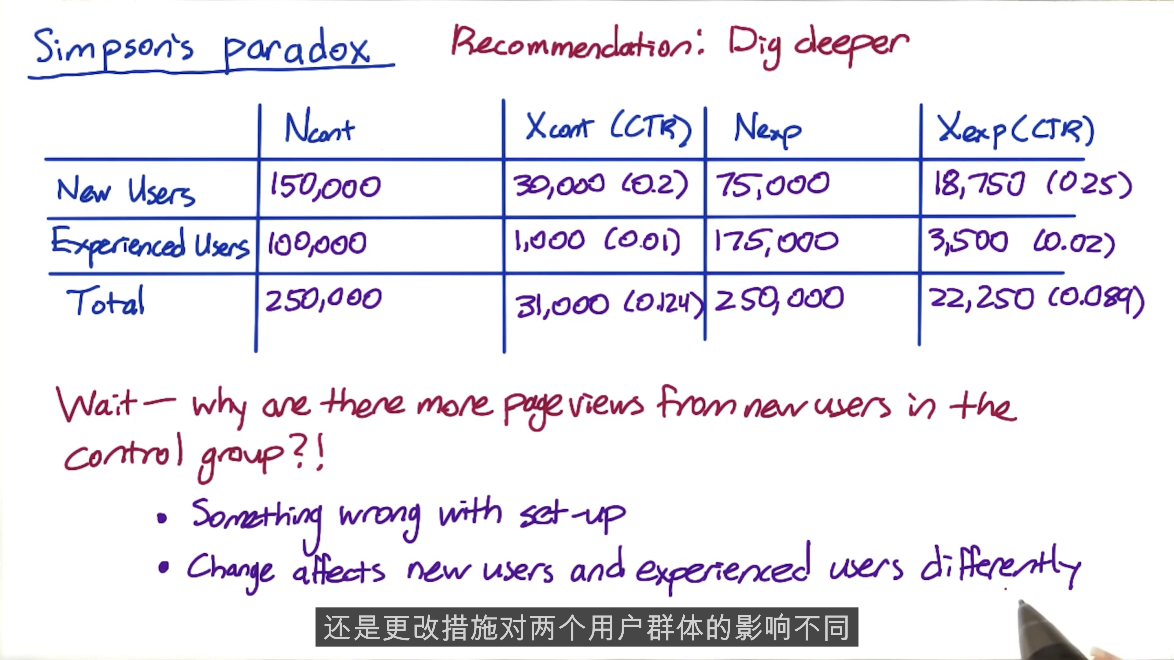
Simpson’s paradox: All subgroups are stable but the integration of them will drives your result.
Within each group, the users behavior is stable; when you mix them together, all the changes in your traffic mix are driving the results.
For example, new users are correlated with weekend use, and experienced users who react differently are correlated with weekday use.
Berkeley example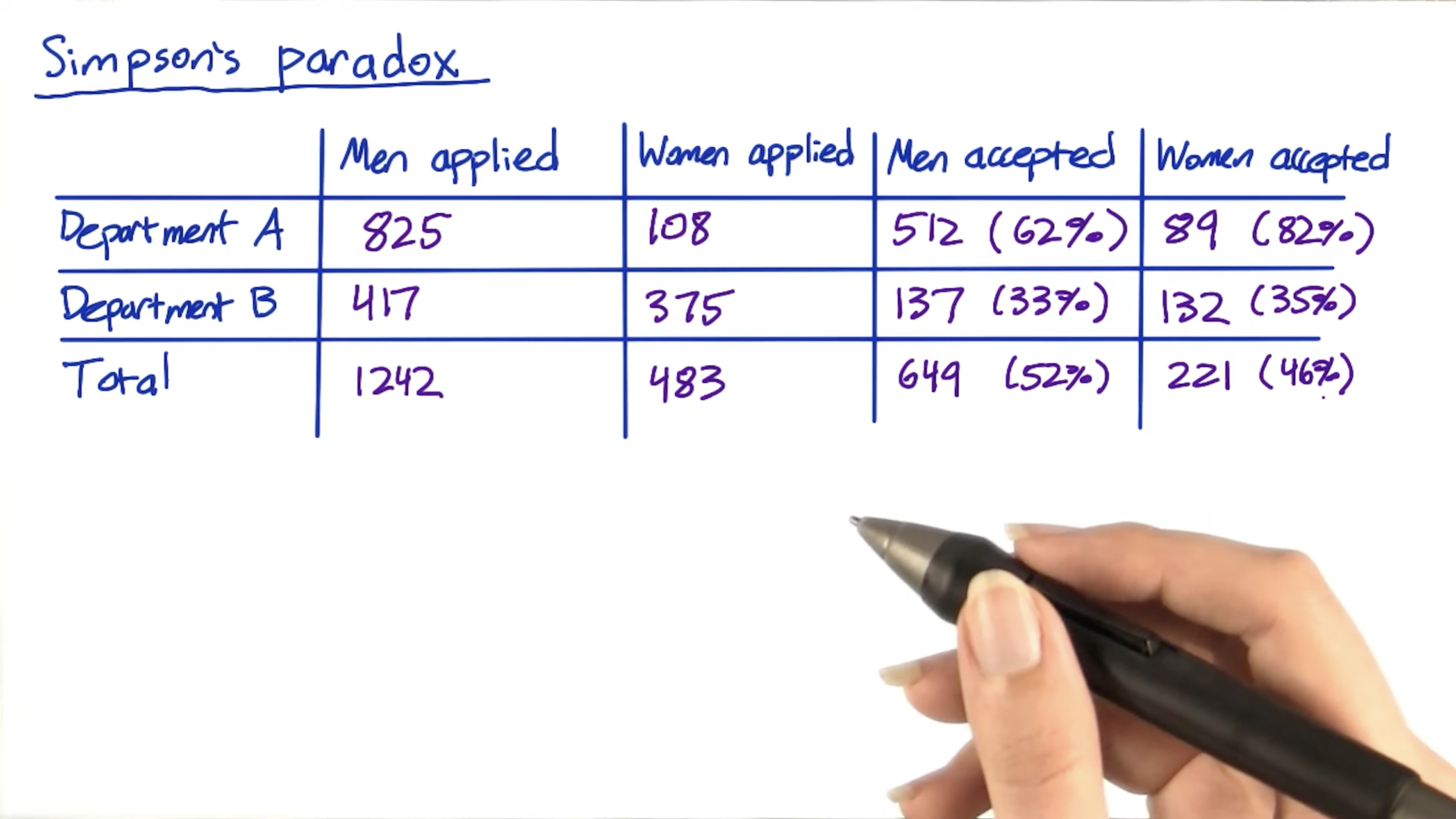
Possible reasons:
- Something wrong with set-up
- Change affects new users and experienced users differently
Recommendation:
- Dig deeper
Multiple Metrics: Introduction
Multiple comparisons
Like Carrie mentioned, as you test more metrics, it becomes more likely that one of them will show a statistically significant result by chance. There will be more details about this in the next videos. You can also find more information in this article.
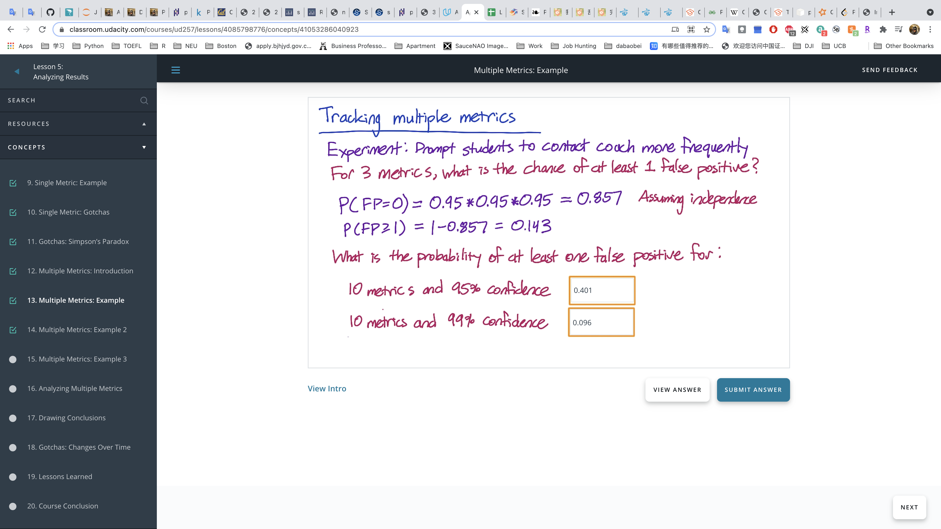
Example 1
Assuming they are independent for calculation.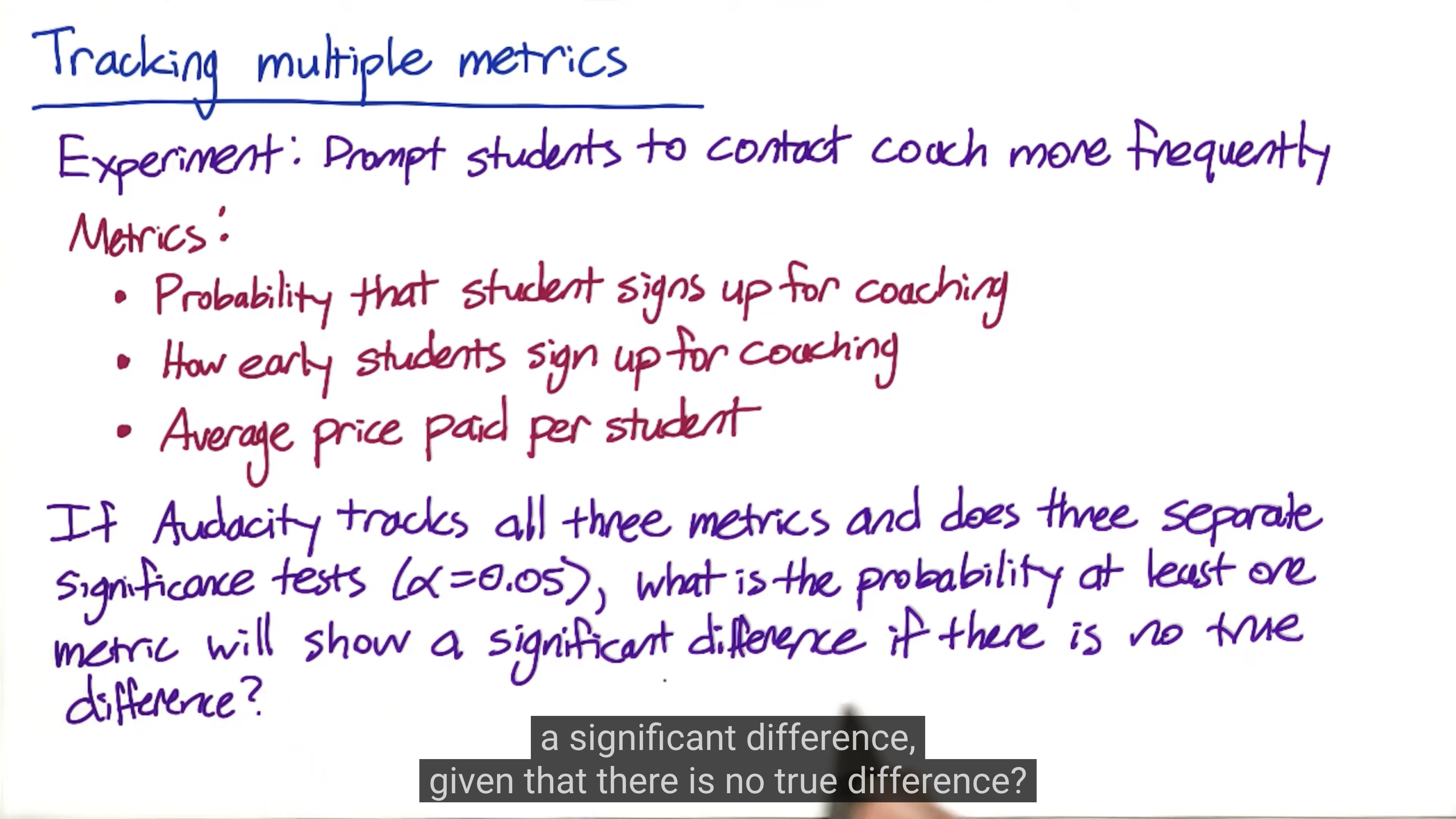
1 | round(1 - 0.95**10, 3) |
Bonferroni correction
You can find more details about the Bonferroni correction, including a proof that it works, in this article.
Tracking multiple metrics
Problem: Probability of any false positive increases as you increase number of metrics
Solution: Use higher confidence level for each metric
Method 1: Assume independence
$\alpha_{overall} = 1 - (1 - \alpha_{individual})^n$
Method 2: Bonferroni correction
- simple
- no assumptions
- too conservative - guaranteed to give $\alpha_{overall}$ at least as small as specified
$\alpha_{individual} = \frac{\alpha_{overall}}{n}$
for example:
$\alpha_{overall} = 0.05, n=3 \Rightarrow \alpha_{individual} = 0.0167$
Example
1 | import numpy as numpy |
1 | # Set NumPy printionoptions |
1 | d_hat = np.array([0.03, 0.5, 0.01, 10]) |
Less conservative multiple comparison methods
The Bonferroni correction is a very simple method, but there are many other methods, including the closed testing procedure, the Boole-Bonferroni bound, and the Holm-Bonferroni method. This article on multiple comparisons contains more information, and this article contains more information about the false discovery rate (FDR), and methods for controlling that instead of the familywise error rate (FWER).
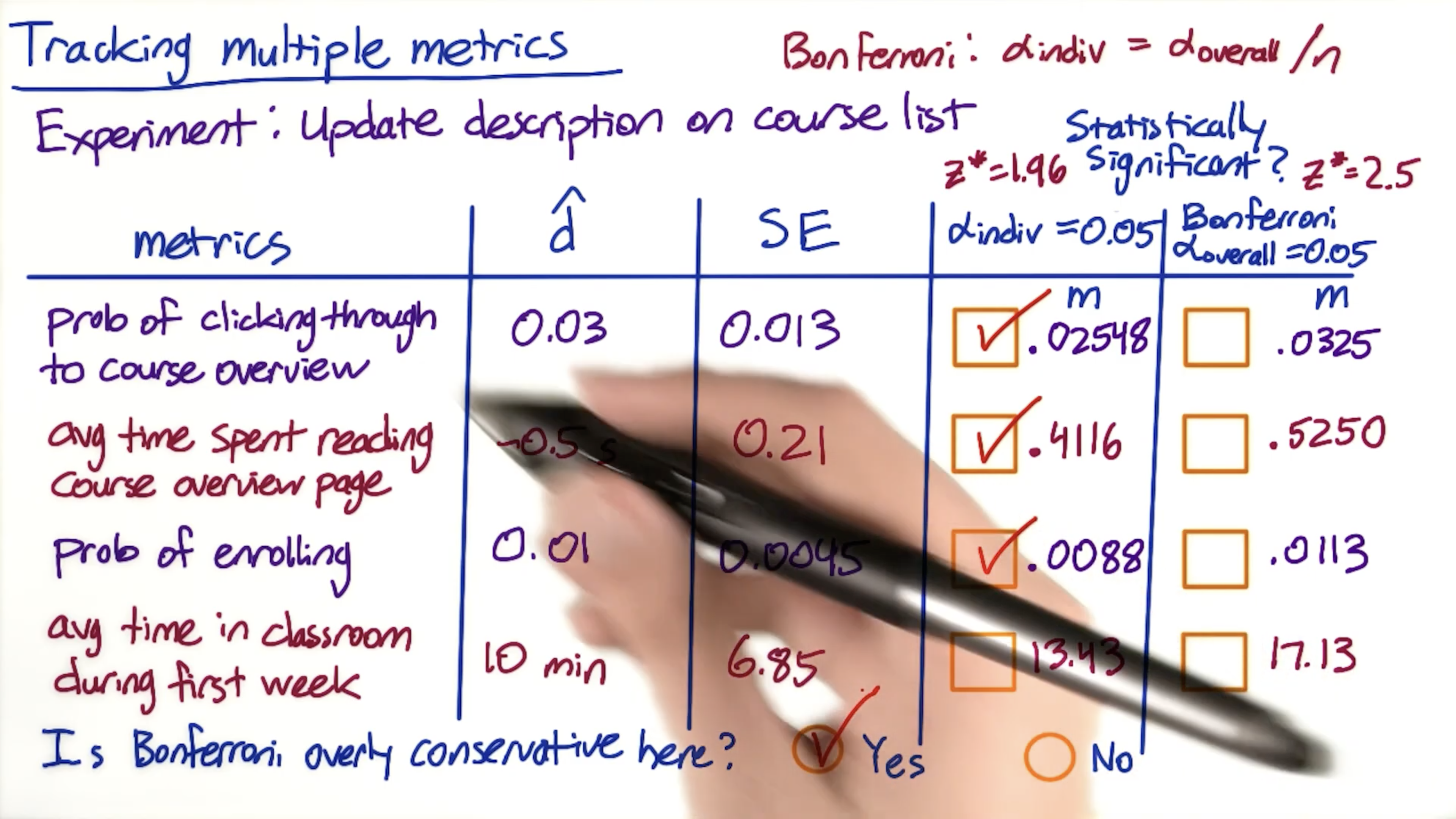
Example
Experiment: Update description on course list
3 out of 4 metrics had significant difference at $\alpha = 0.05$, but non were significant using Bonferroni correction.
Recommendation:
Rigorous answer: Use a more sophisticated method
In practice: Judgment call, possibly based on business strategy
If I have a lot of experience running different experiments with these metrics, then I would have a good intuition for whether these results are likely to persist or not.
In this case, I would need to communicate that to the decision makers to make sure they understand the risk.
Different strategies:
- Control probability that any metric shows a fake positive
$\alpha_{overall}$, familywise error rate (FWER) - Control false discovery rate (FDR)
$FDR = E[\frac{\mbox{false positives}}{\mbox{rejections}}]$
Suppose you have 200 metrics, cap FDR at 0.05. This means you’re okay with 5 false positives and 95 true positives in every experiment.
Analyzing Multiple Metrics
RPM: Revenue per thousand queries
OEC doesn’t have to be a formal number. It’s really just trying to encapsulate what your company cares about. And how much you’re going to be balancing something like stay time and clicks.
Drawing Conclusions
You really have to ask yourself a few questions before you launch the change.
- Do I have statistically significant and and practically significant results in order to justify the change?
- Do I understand what that change has actually done with regards to user experience?
- Is it worth it?
The key thing to remember is that the end goal is actually making that recommendation that shows your judgement. It’s not about designing the experiment and running it and sizing it properly, and having all of the metric chosen correctly, and all those different things. Those are all signposts towards your end goal of actually making a recommendation. And what’s going to be remembered is, did you recommend to launch it or not and was it the right recommendation?
Making a recommendation
In all of our examples this lesson, we’ve tried not just to determine statistical significance, but actually make a recommendation for how to proceed. The examples in these videos show how to do that using the techniques Diane and Carrie talked about.
- Single Metric: Example
- Multiple Metrics: Example
- Multiple Metrics: Example 2
- Multiple Metrics: Example 3
Gotchas: Change Over Time
A good practice is to always do a ramp-up when you actually want to launch a change.
And during you the testing period, remove all of the filters.
The effect may actually flatten out as you ramp up the change. For example, there’s all sorts of seasonality effects; When students go summer vacation, the behavior across broad swaths of the Internet changes. And when they come back from vacation, it changes again. Now, one way to try and capture these seasonal or event-driven impacts is something that we call a holdback.
And the idea is that you launch your change to everyone except for a small holdback, or, basically, a set of users, that don’t get the change, and you continue comparing their behavior to the control. Now in that case you should see the reverse of the impact that you saw in your experiment. And what you can do is you can track that over time until you’re confident that your results are actually repeatable. And that can really help capture a lot of your seasonal or event-drive impacts.
Other possible reasons:
- Users adapt the change.
Final Project
Formulas
$H_0 = p_{exp} - p_{cont} = 0$
$H_1 = p_{exp} - p_{cont} \neq 0$
$\alpha = P(\mbox{reject null | null true})$
$\beta = P(\mbox{failed to reject | null false})$
For two-tailed test:
$z = z_{1-a/2}$
For one-tailed test:
$z = z_{1-a}$
Hypothesis Testing for One Sample Proportion
Binomial proportion confidence interval
Hypothesis Testing for One Sample Proportion
$H_0: p = p_0$
$H_1: p \neq p_0$
If we have $p$, use $p$ instead of $\hat p$
$\displaystyle \sigma^2 = \hat p(1 - \hat p)$
$\displaystyle SE = \sqrt{\frac{\sigma^2}{n}} = \frac{\sigma}{\sqrt{n}} \Rightarrow \sqrt{\frac{\hat p (1 - \hat p)}{n}}$
$\displaystyle CI = \hat p \pm z \cdot SE \Rightarrow \hat p \pm z\sqrt{\frac{\hat p (1 - \hat p)}{n}}$
Proportion power
$\displaystyle \hat p_{pool}= \frac{X_{cont}+X_{exp}}{N_{cont}+ N_{exp}}$
$\displaystyle SE_{pool} = \sqrt{\hat p_{pool} \times (1-\hat p_{pool}) \times (\frac{1}{N_{cont}}+\frac{1}{N_{exp}})}$
For calculating the minimize sample size of control and experiment, $N_{cont} = N_{exp}= N$, then we have:
$\displaystyle \hat p_{pool} = \frac{X_{cont}+X_{exp}}{N + N} = \frac{X_{cont}}{2N} + \frac{X_{exp}}{2N} = \frac{p_{cont}}{2} + \frac{p_{exp}}{2} = \frac{p_{cont} + p_{exp}}{2}$
Therefore:
$\displaystyle SE_{pool} = \sqrt{\hat p_{pool} \times (1-\hat p_{pool}) \times (\frac{1}{N_{cont}}+\frac{1}{N_{exp}})} = \sqrt{\hat p_{pool} \times (1-\hat p_{pool}) \times (\frac{1}{N} + \frac{1}{N})} = \sqrt{\hat p_{pool} \times (1-\hat p_{pool}) \times \frac{2}{N}}$
In this case, $d_{min}$ is equal to Margin of Error.
$d_{min} = p_{exp} - p_{cont}$
$\displaystyle MOE_{\gamma} = Z_{\gamma} \times SE = d_{min}$
$\displaystyle MOE_{\gamma} = Z_{\gamma} \cdot SE_{pool} \Rightarrow d_{min} = Z_{\gamma} \cdot \sqrt{\hat p_{pool} \times (1-\hat p_{pool}) \times \frac{2}{N}} \Rightarrow d_{min}^2 = Z_{\gamma} \cdot \hat p_{pool} \times (1-\hat p_{pool}) \times \frac{2}{N} \Rightarrow n = \frac{Z_{\gamma}^2 \cdot \hat p_{pool} \cdot (1 - \hat p_{pool}) \cdot 2}{d^2}$
$\displaystyle N = (z_{1-\alpha/2} + z_{1-\beta})^2 \left( \frac{\sigma}{\delta} \right)^2 = \frac{Z_{\gamma}^2 \cdot \hat p_{pool} \cdot (1 - \hat p_{pool}) \cdot 2}{d^2} \Rightarrow \mbox{for two-tailed test}$
$\displaystyle N = (z_{1-\alpha} + z_{1-\beta})^2 \left( \frac{\sigma}{\delta} \right)^2 = \frac{Z_{\gamma}^2 \cdot \hat p_{pool} \cdot (1 - \hat p_{pool}) \cdot 2}{d^2} \Rightarrow \mbox{for one-tailed test}$
$\hat d =\hat p_{exp}-\hat p_{cont}$
$H_0: d = 0 \text{ where } \hat{d} \sim N(0,SE_{pool})$
If the statistic is the sample mean, it is called the standard error of the mean (SEM).
$\displaystyle MOE_{\gamma} = Z_{\gamma} \times SE$
Hypothesis Testing for Two-Sample Proportions
$\displaystyle H_0: P_A - P_B = 0$
$\displaystyle H_1: P_A - P_B = d$
$\displaystyle \hat d = p_2 - p_1$
$\displaystyle \hat p = \frac{x_1 + x_2}{n_1 + n_2}$
$\displaystyle \sigma^2 = \hat p (1 - \hat p)$
$\displaystyle SE = \sqrt{\sigma^2 \cdot (\frac{1}{n_1} + \frac{1}{n_2})}$
$\displaystyle Z_{\gamma} = Z_{1 - \frac{\alpha}{2}}$
$\displaystyle Z_{\gamma} = Z_{1 - \alpha}$
$\displaystyle MOE_{\gamma} = Z_{\gamma} \times SE$
$\displaystyle CI = \hat d \pm MOE_{\gamma}$
Binomial test
$\displaystyle H_0: \pi = \pi_0$
$\displaystyle Pr(X = k) = {n \choose k} p^k (1 - p)^{n-k}$
one-tailed
$\displaystyle p = \sum^k_{i=0} Pr(X = i) = \sum^k_{i=0} {n \choose i} p^k (1 - p)^{n-i}$
two-tailed
$\displaystyle p = \sum_{i \in \mathcal{I}} Pr(X = i) = \sum_{i \in \mathcal{I}} {n \choose i} p^k (1 - p)^{n-i}$