AWS Redshift
Introduction
Analyze all of your data with the fastest and most widely used cloud data warehouse
Analyze all of your data
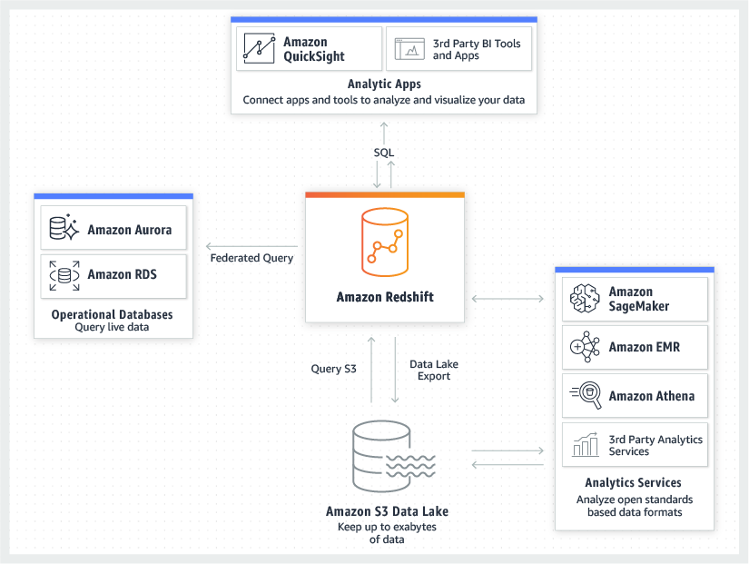
No other data warehouse makes it as easy to gain new insights from all your data. With Redshift, you can query and combine exabytes of structured and semi-structured data across your data warehouse, operational database, and data lake using standard SQL. Redshift lets you easily save the results of your queries back to your S3 data lake using open formats, like Apache Parquet, so that you can do additional analytics from other analytics services like Amazon EMR, Amazon Athena, and Amazon SageMaker.
Redshift Basic Features
- Enterprise-class data warehouse and relational database query and management system
- Connect using many types of client applications
- Business Intelligence (BI)
- Reporting
- Analytics
- Build multi-stage query operations that retrieve, compare, and evaluate large amounts of data
- Efficient storage and optimum query performance
- Massively parallel processing
- Columnar data storage
- Very efficient, targeted data compression encoding schemes
Notice that Redshift stores data as columns, not like normal relational database storing data in rows.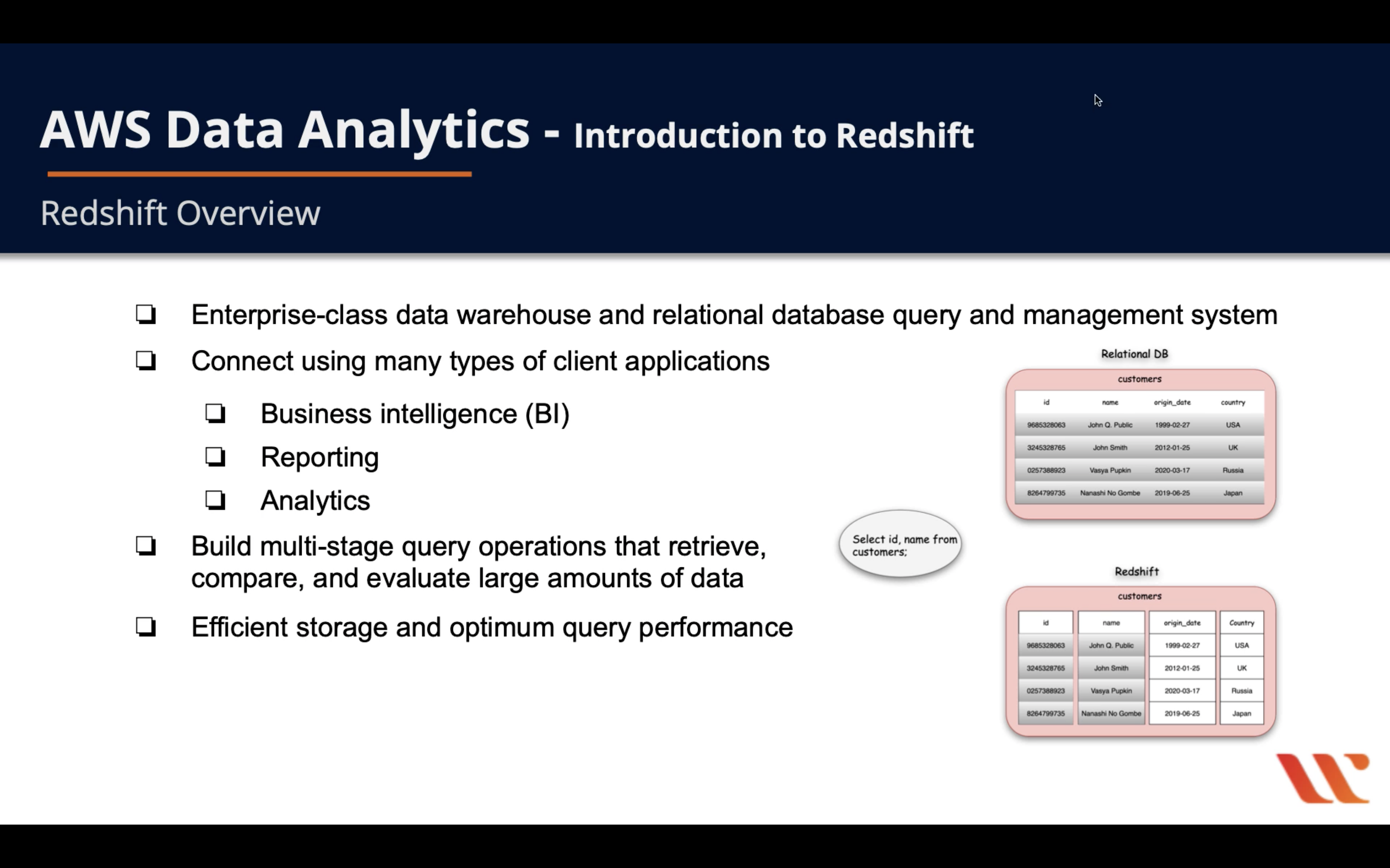
Redshift Architecture
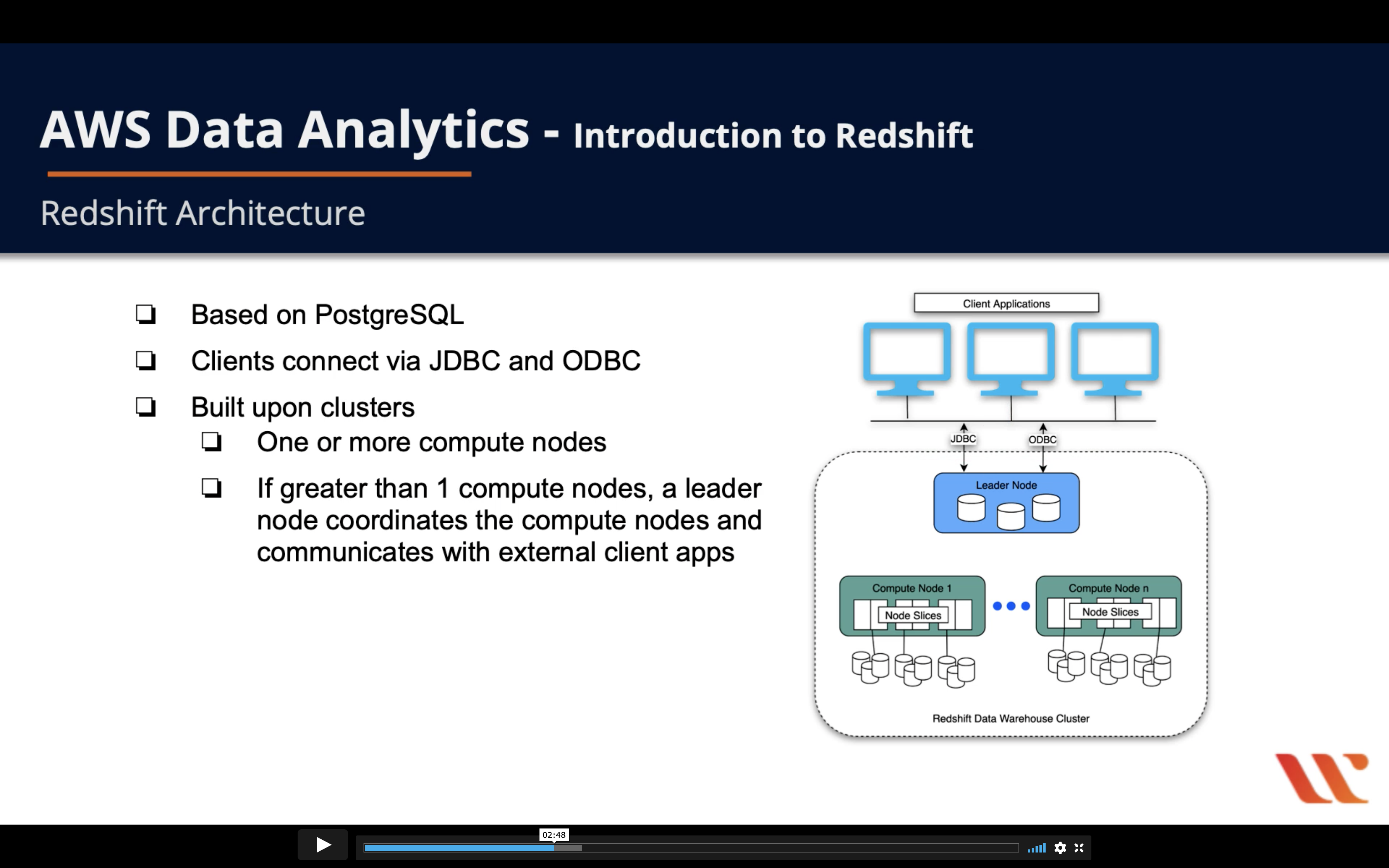
- Based on PostgreSQL
- Clients connect via JDBC and ODBC
- Built upon clusters
- One or more compute nodes
- If greater than 1 compute nodes, a leader node coordinates the compute nodes and communicates with external client apps
Leader Node & Compute Nodes
- Leader node
- Build execution plans to execute database operations - complex queries
- Compiles code and distributes it to the compute nodes, also assigns a portion of the data to each compute node
- Compute node
- Executes the compiled code and sends intermediate results back to the leader node for final aggregation
- Has dedicated CPU, memory, and attached disk storage, which are determined by the node type
- Node types: RA3, DC2, DS2
Node Slices
- Node Slices
- Compute node are partitioned into slices
- Slices are allocated a portion of the node’s memory and disk space
- Processes a part of the workload assigned to the node
- Leader node distributes data to the slices, divides query workload to the slices
- Slices work in parallel to compute your queries
- Assign a column as a distribution key when you create your table on Redshift
- When you load data into your table, rows are distributed to the node slices by the table distribution key - facilitates parallel processing
Columnar Storage
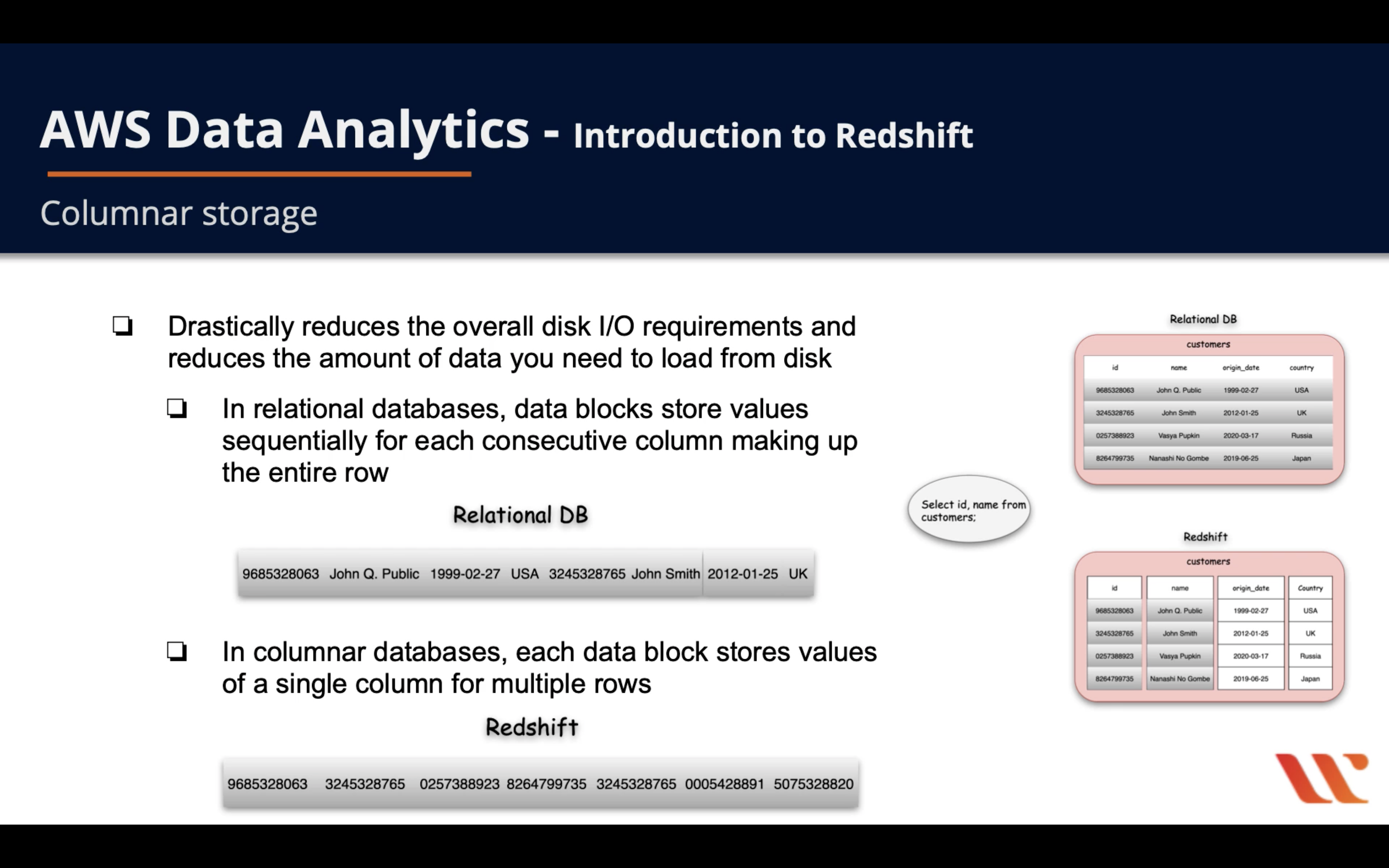
- Drastically reduces the overall disk I/O requirements and reduces the amount of data you need to load from disk
- In relational databases, data blocks store values sequentially for each consecutive column making up the entire row
- In columnar databases, each data block stores values of a single column for multiple rows
- 4~5 times better performance
Data Write & Read
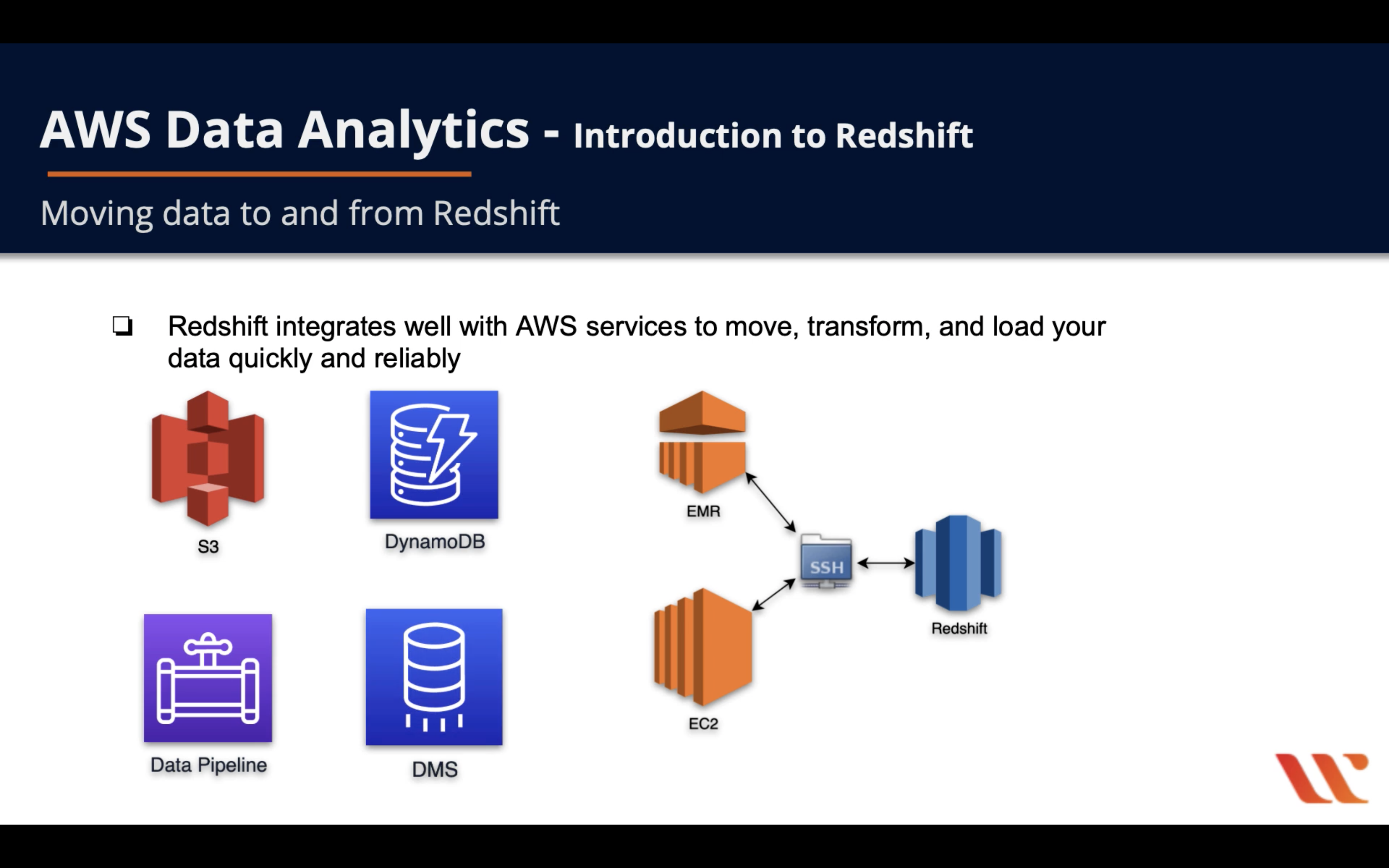
- Redshift integrates well with AWS services to move, transform, and load your data quickly and reliably
Performance
CPU
Memory
Storage
IOPS
Manageability
Security
Access Control
Encryption
Encryption at-rest
Amazon Redshift database encryption
Copying AWS KMS–encrypted snapshots to another AWS Region
Copying snapshots to another AWS Region
Copying AWS KMS–encrypted snapshots to another AWS Region
After a snapshot is copied to the destination AWS Region, it becomes active and available for restoration purposes.
To copy snapshots for AWS KMS–encrypted clusters to another AWS Region, create a grant for Amazon Redshift to use a KMS customer master key (CMK) in the destination AWS Region. Then choose that grant when you enable copying of snapshots in the source AWS Region. For more information about configuring snapshot copy grants, see Copying AWS KMS–encrypted snapshots to another AWS Region.
Note:
If you enable copying of snapshots from an encrypted cluster and use AWS KMS for your master key, you cannot rename your cluster because the cluster name is part of the encryption context. If you must rename your cluster, you can disable copying of snapshots in the source AWS Region, rename the cluster, and then configure and enable copying of snapshots again.
The process to configure the grant for copying snapshots is as follows.
- In the destination AWS Region, create a snapshot copy grant by doing the following:
- If you do not already have an AWS KMS key to use, create one. For more information about creating AWS KMS keys, see Creating Keys in the AWS Key Management Service Developer Guide.
- Specify a name for the snapshot copy grant. This name must be unique in that AWS Region for your AWS account.
- Specify the AWS KMS key ID for which you are creating the grant. If you do not specify a key ID, the grant applies to your default key.
- In the source AWS Region, enable copying of snapshots and specify the name of the snapshot copy grant that you created in the destination AWS Region.
Before the snapshot is copied to the destination AWS Region, Amazon Redshift decrypts the snapshot using the master key in the source AWS Region and re-encrypts it temporarily using a randomly generated RSA key that Amazon Redshift manages internally. Amazon Redshift then copies the snapshot over a secure channel to the destination AWS Region, decrypts the snapshot using the internally managed RSA key, and then re-encrypts the snapshot using the master key in the destination AWS Region.
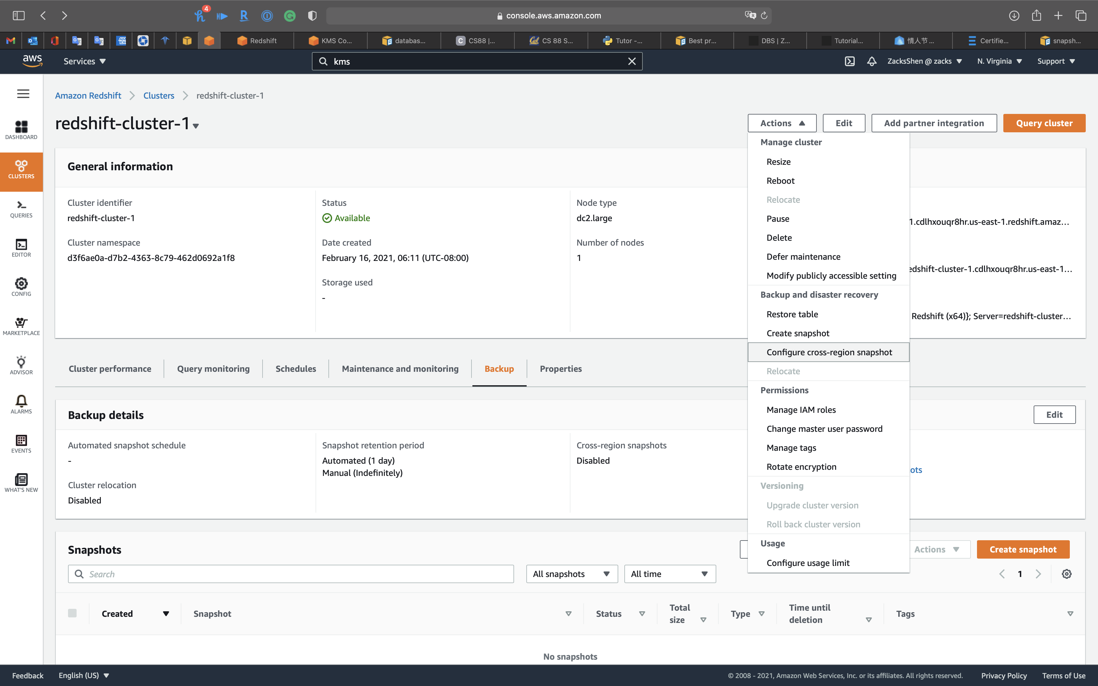
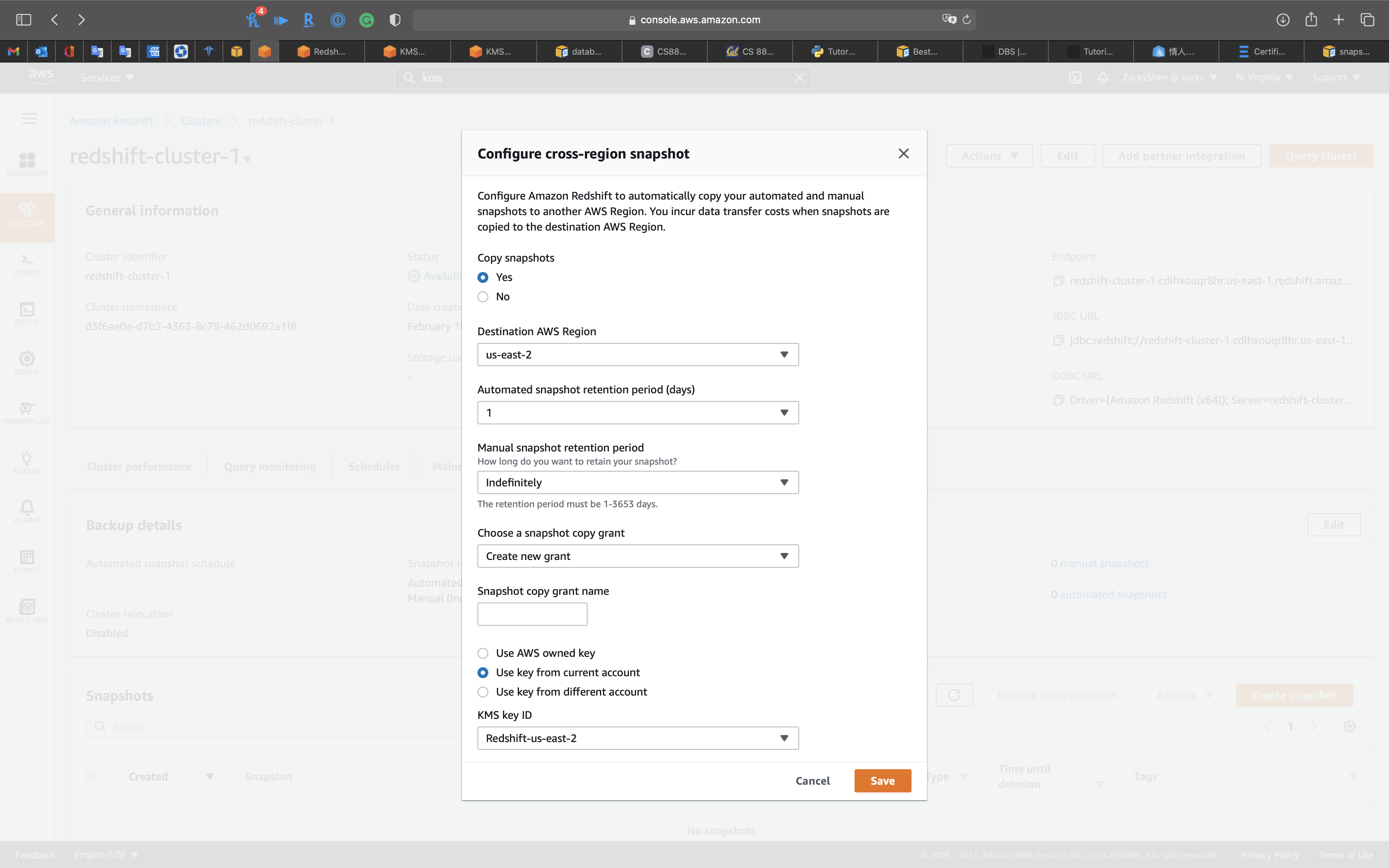
The following example shows copy a snapshot of Redshift cluster in us-east-1 to us-east-2 and grant the copy
- Create a new KMS customer master key in the destination Region and create a new IAM role with access to the new KMS key.
- Enable Amazon Redshift cross-Region replication in the source Region and use the KMS key of the destination Region.
Availability and Durability
Automated Backup
Manual Snapshot
Multi-AZs
Read Replica
Diaster Recovery
RTO & RPO
Disaster Recovery (DR) Objectives
Plan for Disaster Recovery (DR)
Implementing a disaster recovery strategy with Amazon RDS
| Feature | RTO | RPO | Cost | Scope |
|---|---|---|---|---|
| Automated backups(once a day) | Good | Better | Low | Single Region |
| Manual snapshots | Better | Good | Medium | Cross-Region |
| Read replicas | Best | Best | High | Cross-Region |
In addition to availability objectives, your resiliency strategy should also include Disaster Recovery (DR) objectives based on strategies to recover your workload in case of a disaster event. Disaster Recovery focuses on one-time recovery objectives in response natural disasters, large-scale technical failures, or human threats such as attack or error. This is different than availability which measures mean resiliency over a period of time in response to component failures, load spikes, or software bugs.
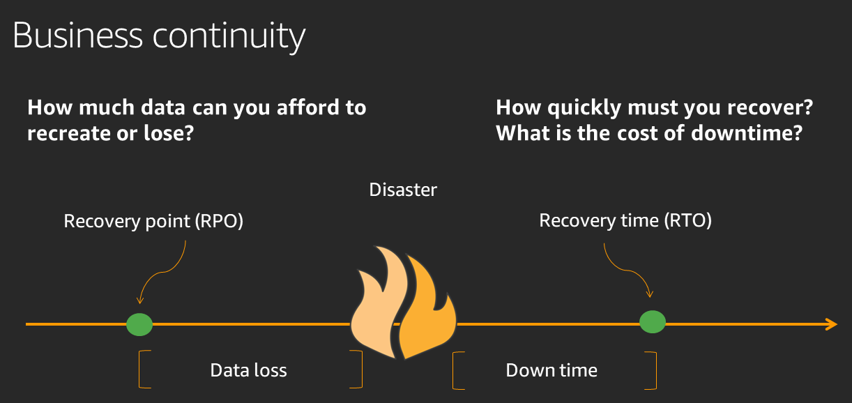
Define recovery objectives for downtime and data loss: The workload has a recovery time objective (RTO) and recovery point objective (RPO).
- Recovery Time Objective (RTO) is defined by the organization. RTO is the maximum acceptable delay between the interruption of service and restoration of service. This determines what is considered an acceptable time window when service is unavailable.
- Recovery Point Objective (RPO) is defined by the organization. RPO is the maximum acceptable amount of time since the last data recovery point. This determines what is considered an acceptable loss of data between the last recovery point and the interruption of service.
Recovery Strategies
Use defined recovery strategies to meet the recovery objectives: A disaster recovery (DR) strategy has been defined to meet objectives. Choose a strategy such as: backup and restore, active/passive (pilot light or warm standby), or active/active.
When architecting a multi-region disaster recovery strategy for your workload, you should choose one of the following multi-region strategies. They are listed in increasing order of complexity, and decreasing order of RTO and RPO. DR Region refers to an AWS Region other than the one primary used for your workload (or any AWS Region if your workload is on premises).
- Backup and restore (RPO in hours, RTO in 24 hours or less): Back up your data and applications using point-in-time backups into the DR Region. Restore this data when necessary to recover from a disaster.
- Pilot light (RPO in minutes, RTO in hours): Replicate your data from one region to another and provision a copy of your core workload infrastructure. Resources required to support data replication and backup such as databases and object storage are always on. Other elements such as application servers are loaded with application code and configurations, but are switched off and are only used during testing or when Disaster Recovery failover is invoked.
- Warm standby (RPO in seconds, RTO in minutes): Maintain a scaled-down but fully functional version of your workload always running in the DR Region. Business-critical systems are fully duplicated and are always on, but with a scaled down fleet. When the time comes for recovery, the system is scaled up quickly to handle the production load. The more scaled-up the Warm Standby is, the lower RTO and control plane reliance will be. When scaled up to full scale this is known as a Hot Standby.
- Multi-region (multi-site) active-active (RPO near zero, RTO potentially zero): Your workload is deployed to, and actively serving traffic from, multiple AWS Regions. This strategy requires you to synchronize data across Regions. Possible conflicts caused by writes to the same record in two different regional replicas must be avoided or handled. Data replication is useful for data synchronization and will protect you against some types of disaster, but it will not protect you against data corruption or destruction unless your solution also includes options for point-in-time recovery. Use services like Amazon Route 53 or AWS Global Accelerator to route your user traffic to where your workload is healthy. For more details on AWS services you can use for active-active architectures see the AWS Regions section of Use Fault Isolation to Protect Your Workload.
Recommendation
The difference between Pilot Light and Warm Standby can sometimes be difficult to understand. Both include an environment in your DR Region with copies of your primary region assets. The distinction is that Pilot Light cannot process requests without additional action taken first, while Warm Standby can handle traffic (at reduced capacity levels) immediately. Pilot Light will require you to turn on servers, possibly deploy additional (non-core) infrastructure, and scale up, while Warm Standby only requires you to scale up (everything is already deployed and running). Choose between these based on your RTO and RPO needs.
Tips
Test disaster recovery implementation to validate the implementation: Regularly test failover to DR to ensure that RTO and RPO are met.
A pattern to avoid is developing recovery paths that are rarely executed. For example, you might have a secondary data store that is used for read-only queries. When you write to a data store and the primary fails, you might want to fail over to the secondary data store. If you don’t frequently test this failover, you might find that your assumptions about the capabilities of the secondary data store are incorrect. The capacity of the secondary, which might have been sufficient when you last tested, may be no longer be able to tolerate the load under this scenario. Our experience has shown that the only error recovery that works is the path you test frequently. This is why having a small number of recovery paths is best. You can establish recovery patterns and regularly test them. If you have a complex or critical recovery path, you still need to regularly execute that failure in production to convince yourself that the recovery path works. In the example we just discussed, you should fail over to the standby regularly, regardless of need.
Manage configuration drift at the DR site or region: Ensure that your infrastructure, data, and configuration are as needed at the DR site or region. For example, check that AMIs and service quotas are up to date.
AWS Config continuously monitors and records your AWS resource configurations. It can detect drift and trigger AWS Systems Manager Automation to fix it and raise alarms. AWS CloudFormation can additionally detect drift in stacks you have deployed.
Automate recovery: Use AWS or third-party tools to automate system recovery and route traffic to the DR site or region.
Based on configured health checks, AWS services, such as Elastic Load Balancing and AWS Auto Scaling, can distribute load to healthy Availability Zones while services, such as Amazon Route 53 and AWS Global Accelerator, can route load to healthy AWS Regions.
For workloads on existing physical or virtual data centers or private clouds CloudEndure Disaster Recovery, available through AWS Marketplace, enables organizations to set up an automated disaster recovery strategy to AWS. CloudEndure also supports cross-region / cross-AZ disaster recovery in AWS.
Migration
Monitoring
Redshift Data Storage and Retrieval Patterns
Redshift Node Types
- Three different node types: RA3, DC2, DS2
- Node type defines CPU, memory, storage capacity and drive type
RA3
- RA3: compute and manged storage independently
- Managed storage
- Optimize by scaling and paying for compute and manged storage independently
- Select number of nodes for your performance requirements; pay for the manged storage that you use
- Configure RA3 cluster based on daily amount of processed data
- Launch RA3 node type clusters in VPC
- RA3s use SSD for fast local storage and S3 for longer-term durable storage
- If node data outgrows the size of local SSDs, Redshift managed storage automatically offloads that data to S3
- Scale storage capacity without adding and paying for additional nodes
- Use high bandwidth networking built on the AWS Nitro System
- RA3 scenarios
- Scale compute separate from storage
- Typically query a small amount of your total data
- Data volume growing quickly or is expected to grow quickly
- Size cluster based on performance needs
DC2
- DC2: compute and manged storage dependently
- Compute-intensive warehouse with local SSD storage included
- Choose the number of nodes needed for data size and performance requirements (cannot manage the storage separately)
- Store data locally for high performance
- When data requirements increase, add more compute nodes to increase the storage capacity of the cluster
- Recommended for datasets under 1 TB (compressed), for best price and performance
- If data is expected to grow, use RA3 to take advantage of sizing compute and storage separately for best price and performance
- Launch DC2 node type clusters in VPC
DS2
- DS2: legacy
- Build large data warehouses using HDDs
- AWS recommends using RA3 nodes instead
- AWS supplies an upgrade path from DC2 nodes to RA3 nodes
- RA3 nodes give 2x more storage and improved performance for equal cost when using on-demand
Other compute node considerations
- Redshift distributes and executes your queries in parallel across all of your compute nodes
- Increase performance by adding compute nodes
- Clusters with more than one compute node, Redshift mirrors on each node to another node, making data durable
- Increase or decrease nodes for price/performance balance
- When nodes are added, Redshift deploys and load balances for you
- Can purchase reserved nodes to save on cost
Redshift Data Layout, Schema, Structure
Distribution Styles
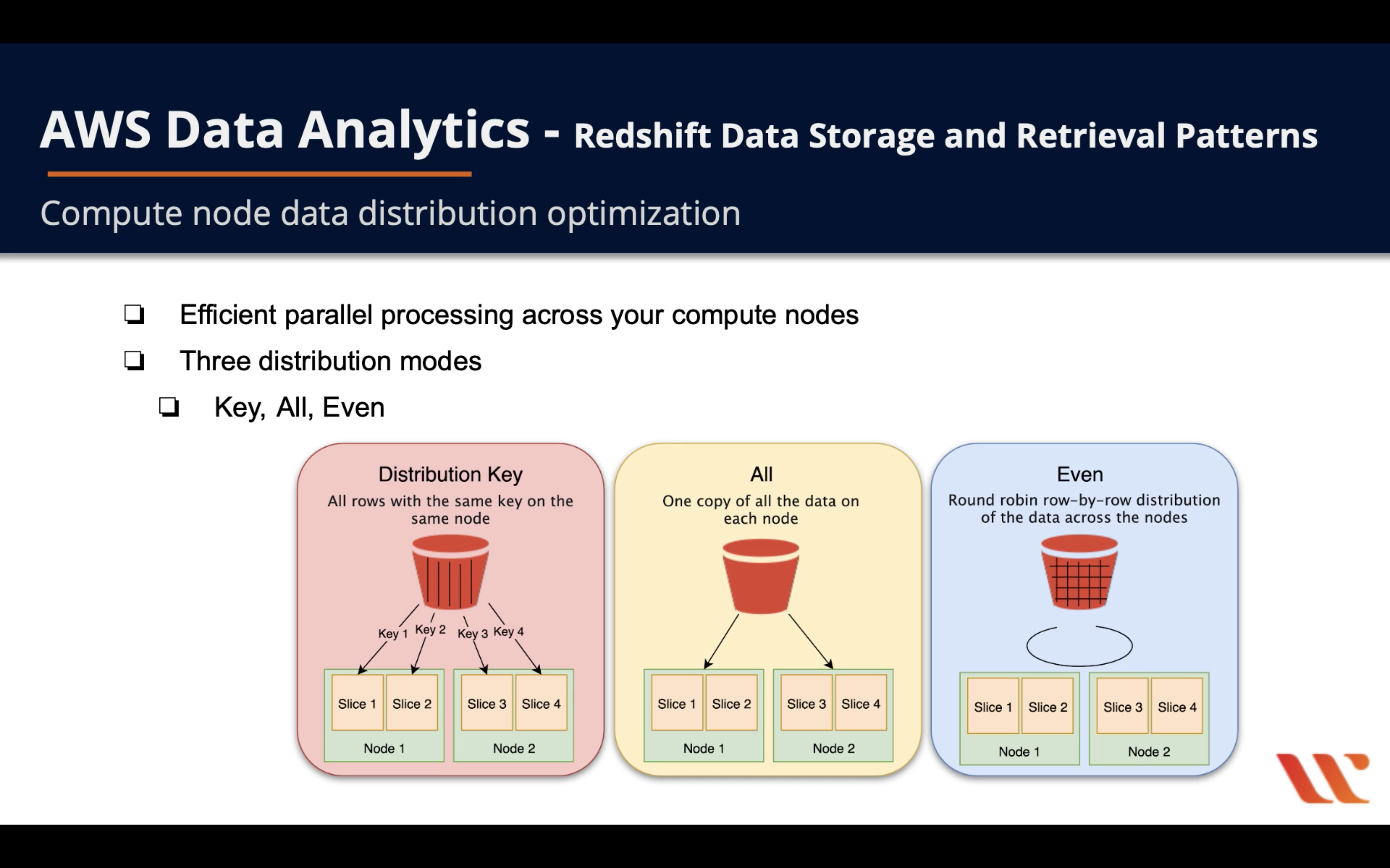
- Efficient parallel processing across your compute nodes
- Three distribution modes
- Key: All rows with the same key on the same node (for huge workload of join)
- All: Once copy of all the data on each node
- Even: Round robin row-by-row distribution of the data across the nodes
AUTO distribution
- With AUTO distribution, Amazon Redshift assigns an optimal distribution style based on the size of the table data. For example, Amazon Redshift initially assigns ALL distribution to a small table, then changes to EVEN distribution when the table grows larger. When a table is changed from ALL to EVEN distribution, storage utilization might change slightly. The change in distribution occurs in the background, in a few seconds.
EVEN distribution
- The leader node distributes the rows across the slices in a round-robin fashion, regardless of the values in any particular column. EVEN distribution is appropriate when a table doesn’t participate in joins. It’s also appropriate when there isn’t a clear choice between KEY distribution and ALL distribution.
KEY distribution
- The rows are distributed according to the values in one column. The leader node places matching values on the same node slice. If you distribute a pair of tables on the joining keys, the leader node collocates the rows on the slices according to the values in the joining columns. This way, matching values from the common columns are physically stored together.
ALL distribution
- A copy of the entire table is distributed to every node. Where EVEN distribution or KEY distribution place only a portion of a table’s rows on each node, ALL distribution ensures that every row is collocated for every join that the table participates in.
Redshift sort keys
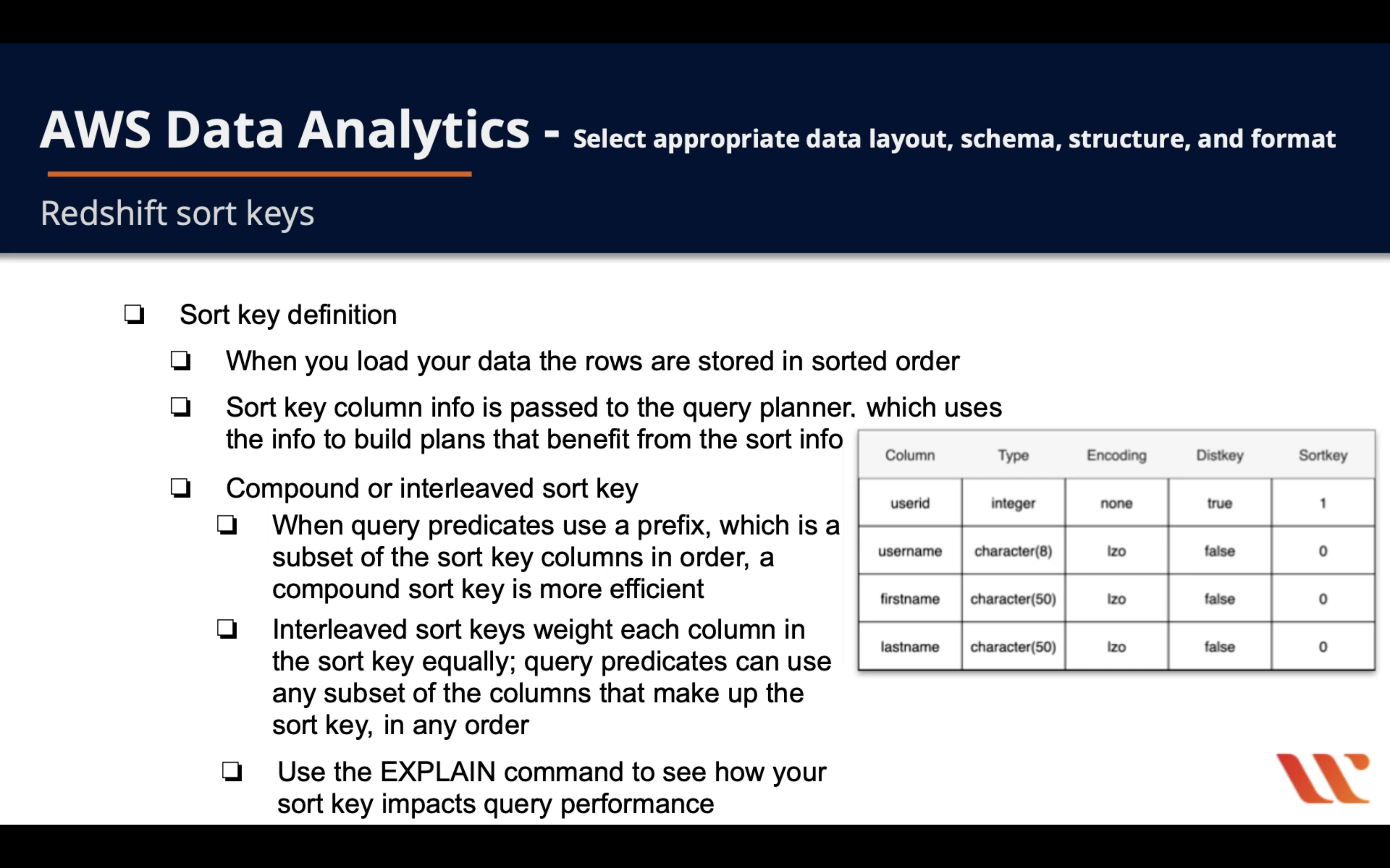
- Sort key definition
- When you load your data the rows are stored in sorted order
- Sort key column info is passed to the query planner, which uses the info to build plans that benefit from the sort info
- Compound or Interleaved sort key
- When query predicates use a prefix, which is a subset of the sort key columns in order, a compound sort key is more efficient
- Interleaved sort keys weight each column in the sort key equally; query predicates can use any subset of the columns that make up the sort key, in any order
- Use the EXPLAIN command to see how your sort key impacts query performance
Redshift COPY Command
- COPY command is the most efficient way to load a Redshift table
- Read from multiple data files or multiple data streams simultaneously
- Redshift assigns the workload to the cluster nodes and loads the data in parallel, including sorting the rows and distributing data across node slices
- Can’t COPY into Redshift Spectrum tables
- Use VACUUM command to reorganize your data in your tables
Redshift Compression Types
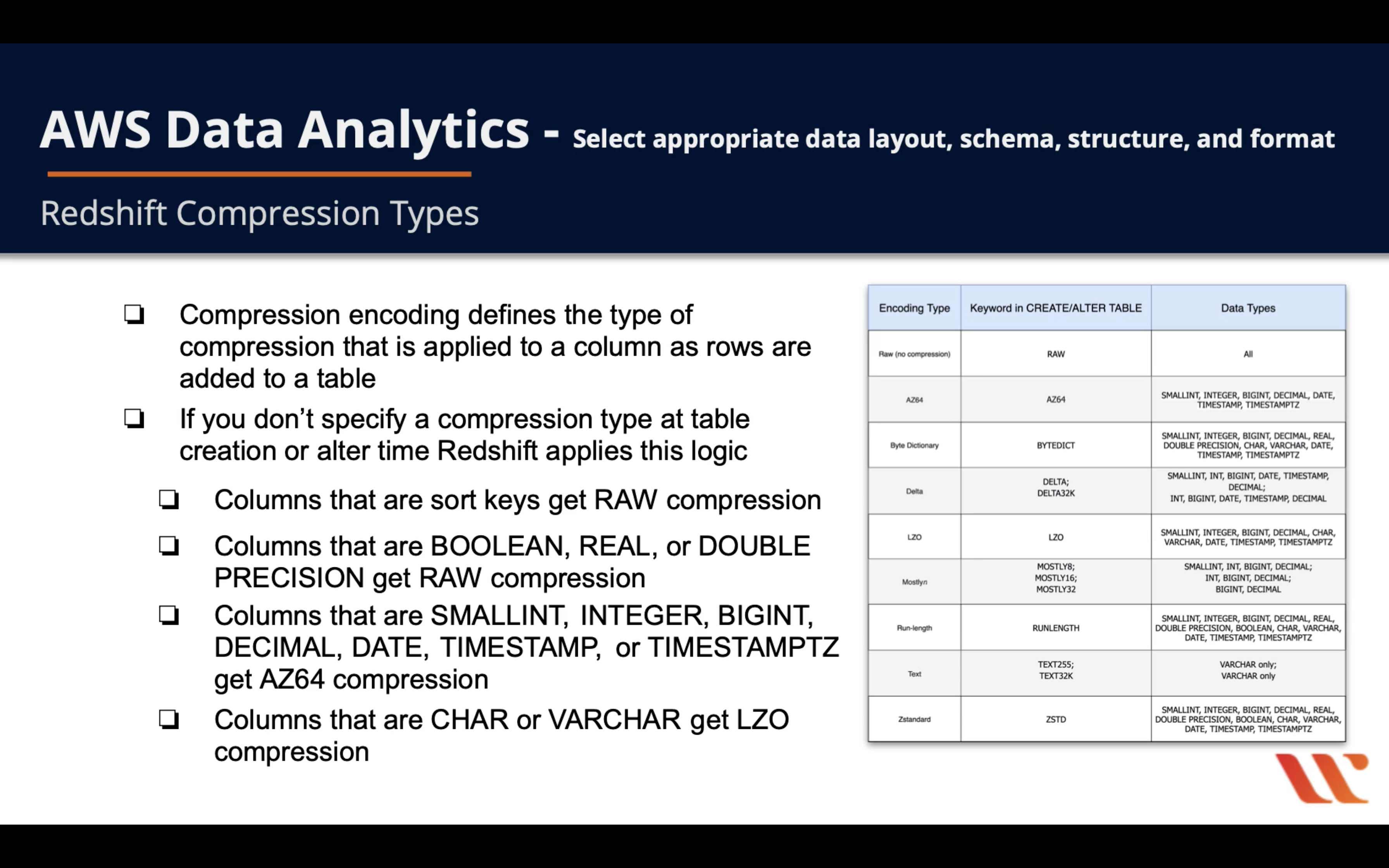
- Compression encoding defines the type of compression that is applied to a column as rows are added to a table
- If you don’t specify a compression type ate table creation or alter time Redshift applies this logic
- Columns that are sort keys get RAW compression
- Columns that are BOOLEAN, REAL, or DOUBLE PRECISION get RAW compression
- Columns that are SMALLINT, INTEGER, BIGINT, DECIMAL, DATE, TIMESTAMP, or TIMESTAMPTZ get AZ64 compression
- Columns that area CHAR or VARCHAR get LZO compression
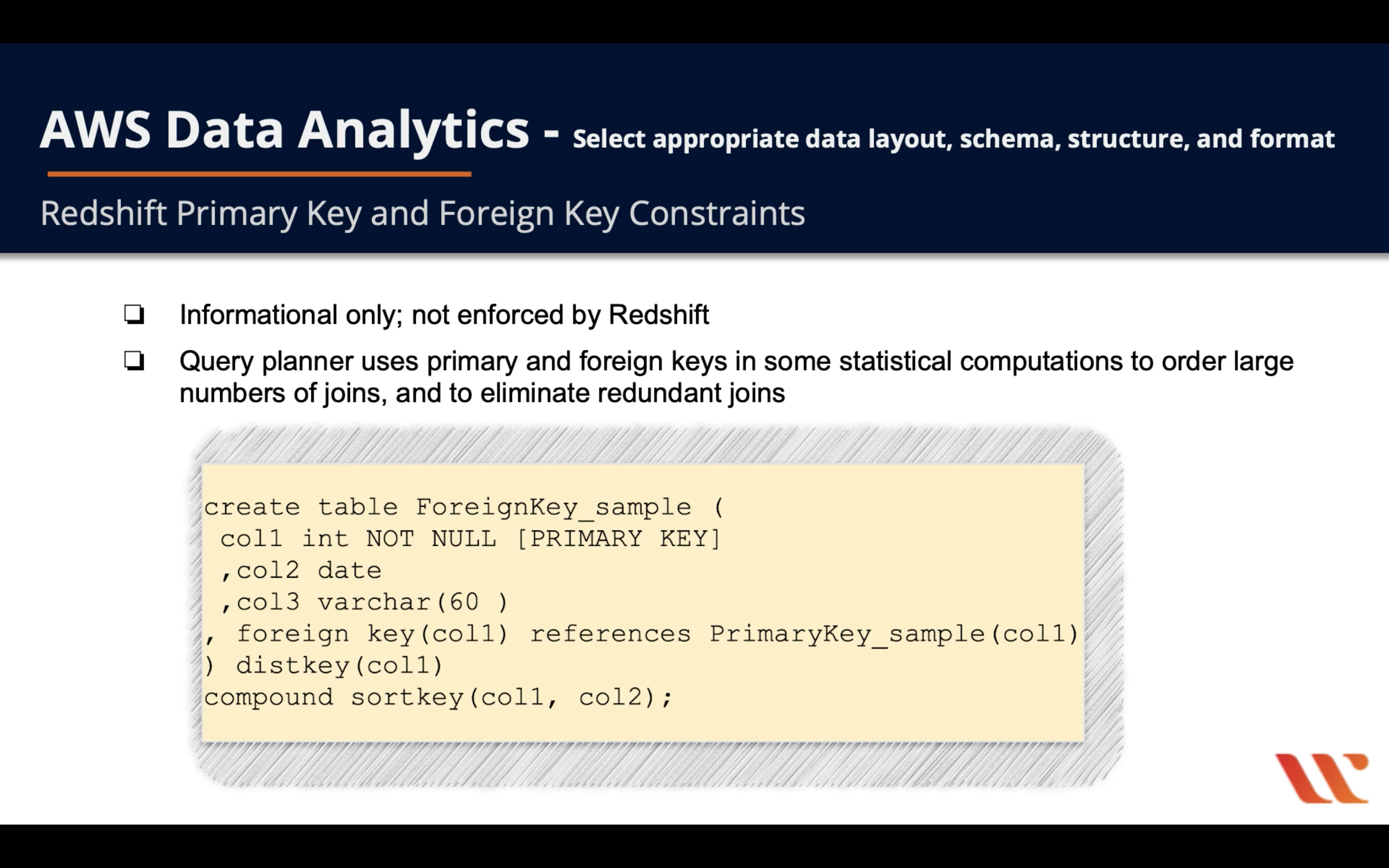
Redshift Primary Key and Foreign Key Constraints
- Informational only; not enforced by Redshift
- Query planner uses primary and foreign keys in some statistical computations to order large number of joins and to eliminate redundant joins.
- Don’t make Primary key and Foreign key constraints unless your application enforce it. Because Redshift doesn’t enforce unique Primary key and Foreign key constraints.