AWS DynamoDB
Introduction
Fast and flexible NoSQL database service for any scale
Amazon DynamoDB
Introduction to AWS DynamoDB Lab
DynamoDB & Global Secondary Index
DynamoDB Global Table & Load Data from S3 Lab
Best Practices for Designing and Using Partition Keys Effectively
AWS Databases for Real-Time Applications
Amazon DynamoDB is a key-value and document database that delivers single-digit millisecond performance at any scale. It’s a fully managed, multi-region, multi-active, durable database with built-in security, backup and restore, and in-memory caching for internet-scale applications. DynamoDB can handle more than 10 trillion requests per day and can support peaks of more than 20 million requests per second.
Many of the world’s fastest growing businesses such as Lyft, Airbnb, and Redfin as well as enterprises such as Samsung, Toyota, and Capital One depend on the scale and performance of DynamoDB to support their mission-critical workloads.
Hundreds of thousands of AWS customers have chosen DynamoDB as their key-value and document database for mobile, web, gaming, ad tech, IoT, and other applications that need low-latency data access at any scale. Create a new table for your application and let DynamoDB handle the rest.
DynamoDB Basic Features
What is AWS DynamoDB?
- Definition
- DynamoDB is a fast and flexible NoSQL database designed for applications that need consistent, single-digit millisecond latency at any scale. It is a fully managed database and it supports both document and key value data models.
- It has a very flexible data model. This means that you don’t need to define your database schema upfront. It also has reliable performance.
- DynamoDB is a good fit for mobile gaming, ad-tech, IoT and many other applications.
DynamoDB Tables
DynamoDB tables consist of
- Items (Think of a row of data in a table).
- Attributes (Think of a column of data in a table).
- Supports key-value and document data structures.
Key= the name of the data.Value= the data itself.Documentcan be written in JSON, HTML or XML.
DynamoDB - Primary Keys
- DynamoDB stores and retrieves data based on a Primary key.
- DynamoDB also uses Partition keys to determine the physical location data is stored.
- If you are using a partition key as your Primary key, then no items will have the same Partition key.
- All items with the same partition key are stored together and then sorted according to the sort key value.
- Composite Keys (Partition Key + Sort Key) can be used in combination.
- Two items may have the same partition key, but must have a different sort key.
What is an Index in DynamoDB
- In SQL databases, an index is a data structure which allows you to perform queries on specific columns in a table.
- You select the column that is required to include in the index and run the searches on the index instead of on the entire dataset.
In DynamoDB, two types of indexes are supported to help speed-up your queries.
- Local secondary Index.
- Global Secondary Index.
Local Secondary Index
- Can only be created when you are creating the table.
- Cannot be removed, added or modified later.
- It has the same partition key as the original table.
- Has a different Sort key.
- Gives you a different view of your data, organized according to an alternate sort key.
- Any queries based on Sort key are much faster using the index than the main table.
Global Secondary Index
- You can create a GSI on creation or you can add it later.
- Different partition key as well as different sort key.
- It gives a completely different view of the data.
- Speeds up the queries relating to this alternative Partition or Sort Key.
| No. | LSI | GSI |
|---|---|---|
| 1 | Key = hash key and a range key | Key = hash or hash-and-range |
| 2 | Hash same attribute as that of the table. Rage key can be any scalar table attribute | The index hash key and range key (if present) can be any scalar table attributes. |
| 3 | For each hash key, the total size of all indexed items must be 10GB or less. | No size restrictions for global secondary indexes. |
| 4 | Query over a single partition, as specified by the hash key value in the query. | Query over the entire table, across all partitions. |
| 5 | Eventual consistency or strong consistency. | Eventual consistency only. |
| 6 | Read and write capacity units consumed from the table. | Every global secondary index has its own provisioned read and write capacity units. |
| 7 | Query will automatically fetch non-projected attributes from the table. | Query can only request projected attributes. It will not fetch attributes from the table. |
Eventual Consistency vs Strong Consistency
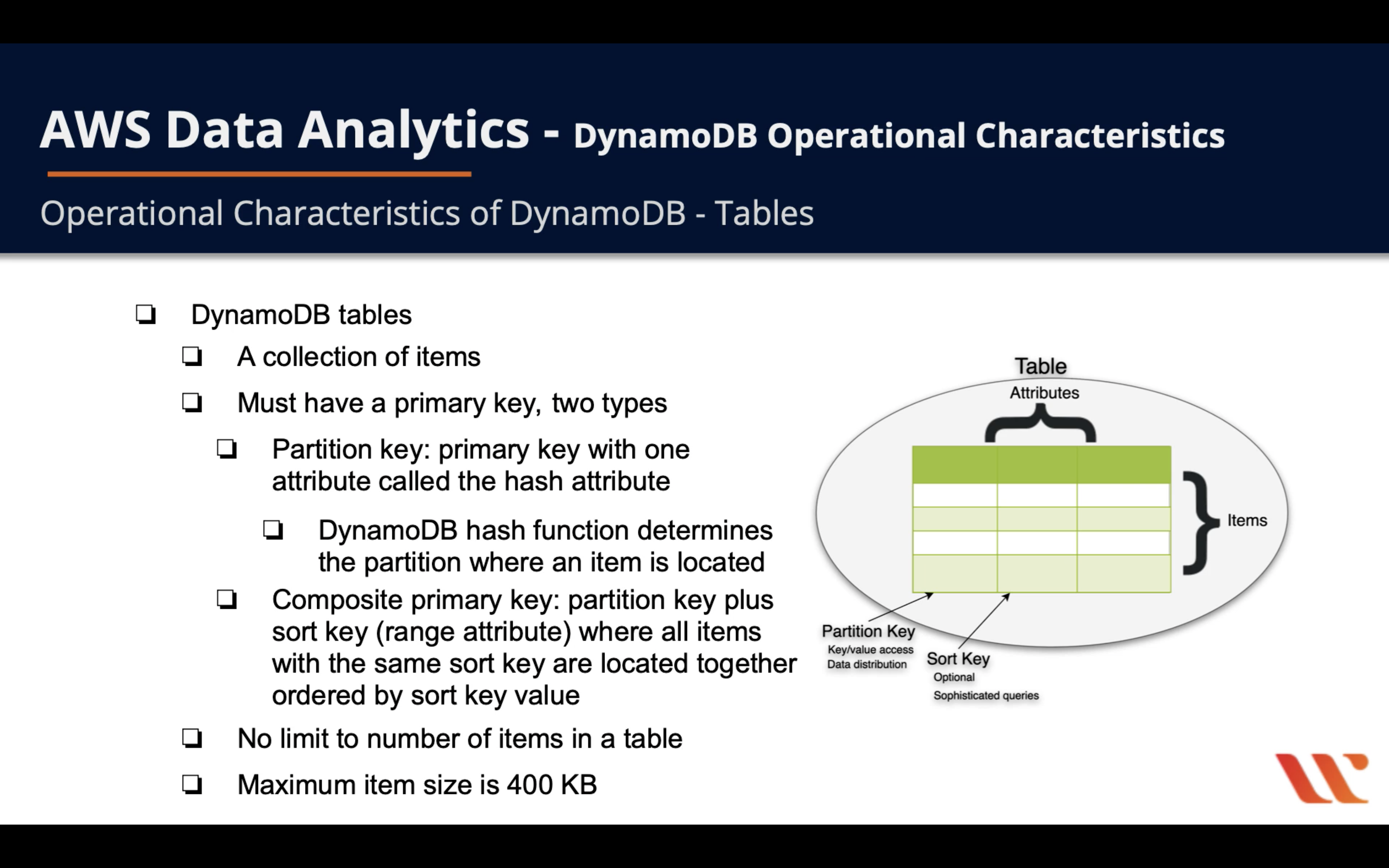
DynamoDB Tables
- DynamoDB Tables
- A collection of items
- Must have a primary key, two types
- Partition key: primary key with one attribute called the hash attribute
- DynamoDB hash function determines the partition where an item is located
- Composite primary key: partition key plus sort key (range attribute) where all items with the same sort key are located together ordered by sort key value
- Partition key: primary key with one attribute called the hash attribute
- No limit to number of items in a table
- Maximum item size is 400 KB
DynamoDB Two Read Models
- DynamoDB: Two Read Modes
- Eventually consistent reads for higher performance but lower accuracy (default)
- Achieves maximum read throughput
- May return stale data
- Strongly consistent reads for lower performance but higher accuracy
- Return result representing all prior write operations
- Always accurate data returned (no stale data)
- Increased latency with this option
- Eventually consistent reads for higher performance but lower accuracy (default)
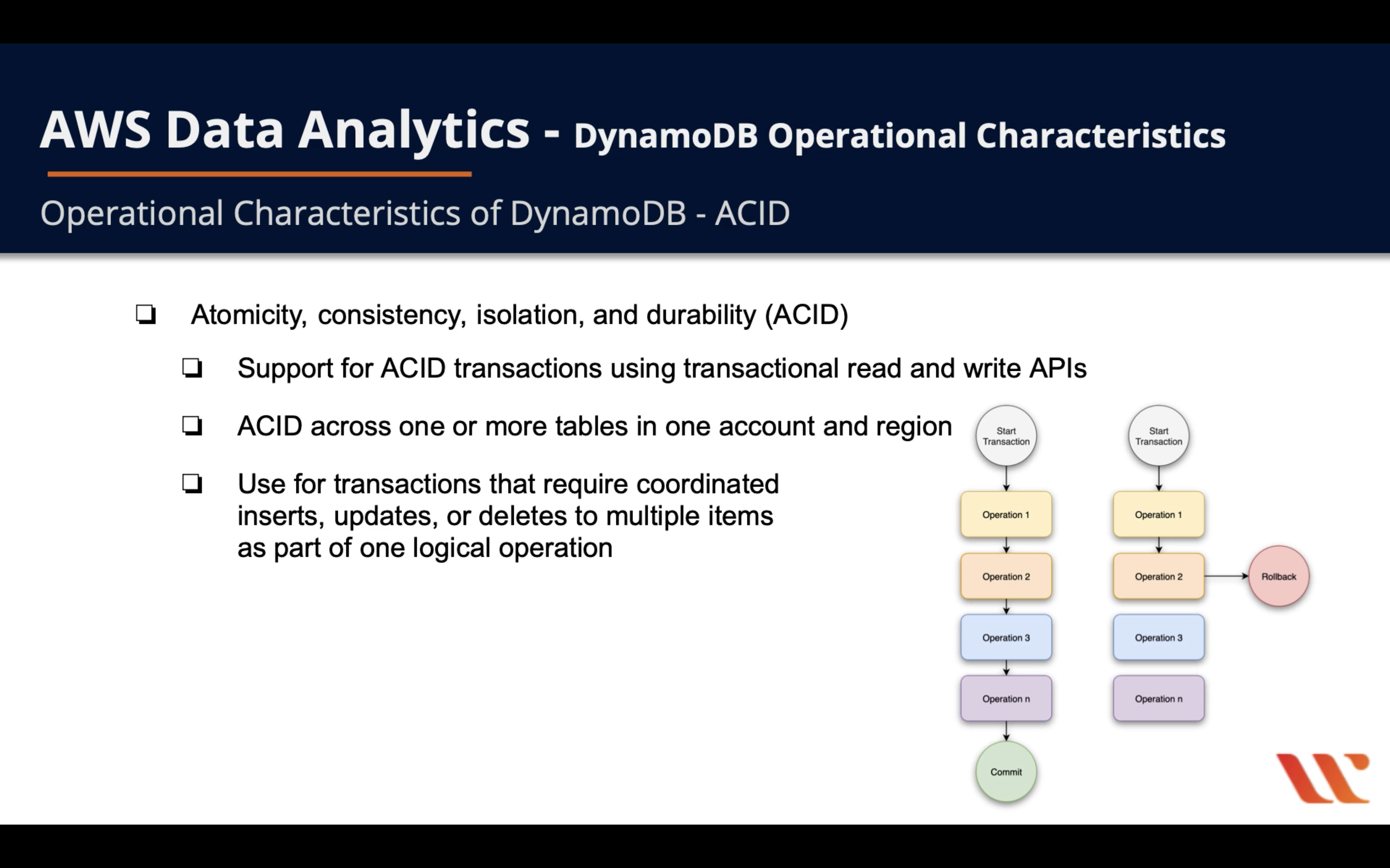
Atomicity, Consistency, Isolation, and Durability (ACID)
- Atomicity, Consistency, Isolation, and Durability (ACID)
- Support operation rollback
- Support for ACID transactions using transactional read and write APIs
- ACID across one or more tables in one account and region
- Use for transactions that require coordinated inserts, updates, or deletes to multiple items as part of one logical operation
Cost vs. Performance - Two Capacity Modes
- Cost vs. Performance - Two Capacity Modes
- On-demand capacity
- DynamoDB automatically provisions capacity based on your workload, up or down
- Provisioned capacity
- Specify read capacity units (RCUs) and write capacity units (WCUs) per second for your application
- For Avg. item size up to 4 KB, every 4 KB of Avg. item will be counted as a coefficient
- 1 RCU = 1 read/sec strongly consistent
- 1 RCU = 2 read/rec eventually consistent
- 2 RCU = 1 read/rec transactional
- For Avg. item size up to 1 KB, every 1 KB of Avg. item will be counted as a coefficient
- 1 WCU = 1 write/sec
- Can use auto scaling to automatically calibrate your table’s capacity
- Helps manage cost
- On-demand capacity
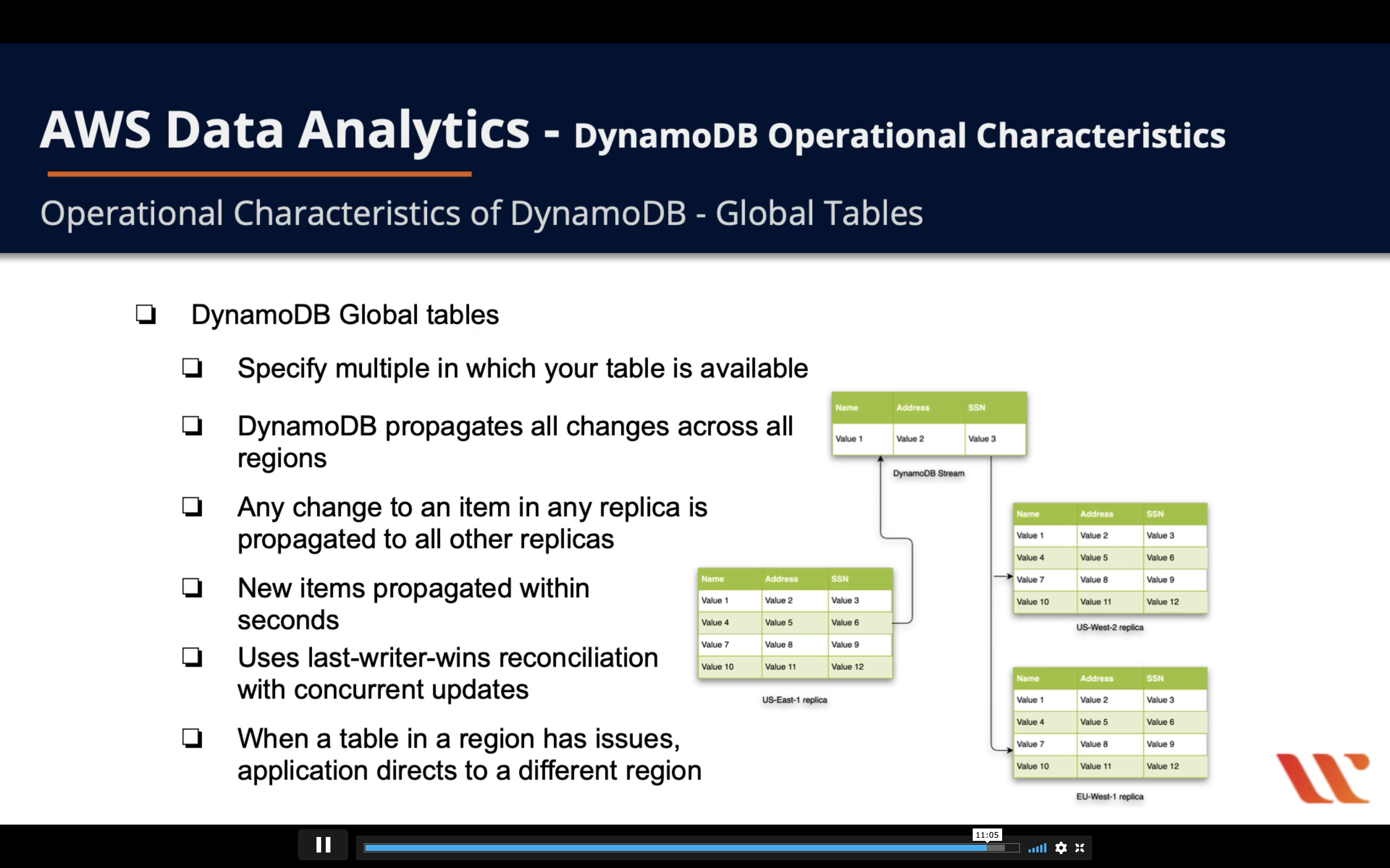
DynamoDB Global Tables
- DynamoDB Global Tables
- Global Table is fully managed service with multi-region and multi-master database delivering fast, local, read, and write performance for massive scaled global applications.
- Specify multiple in which your table is available
- DynamoDB propagates all changes across all regions
- Any change to an item in ay replica is propagated to all other replicas
- New items propagated within seconds
- Uses last-writer-wins reconciliation with concurrent update
- When a table in a region has issues, application directs to a different region
DynamoDB Layout, Schema, Structure
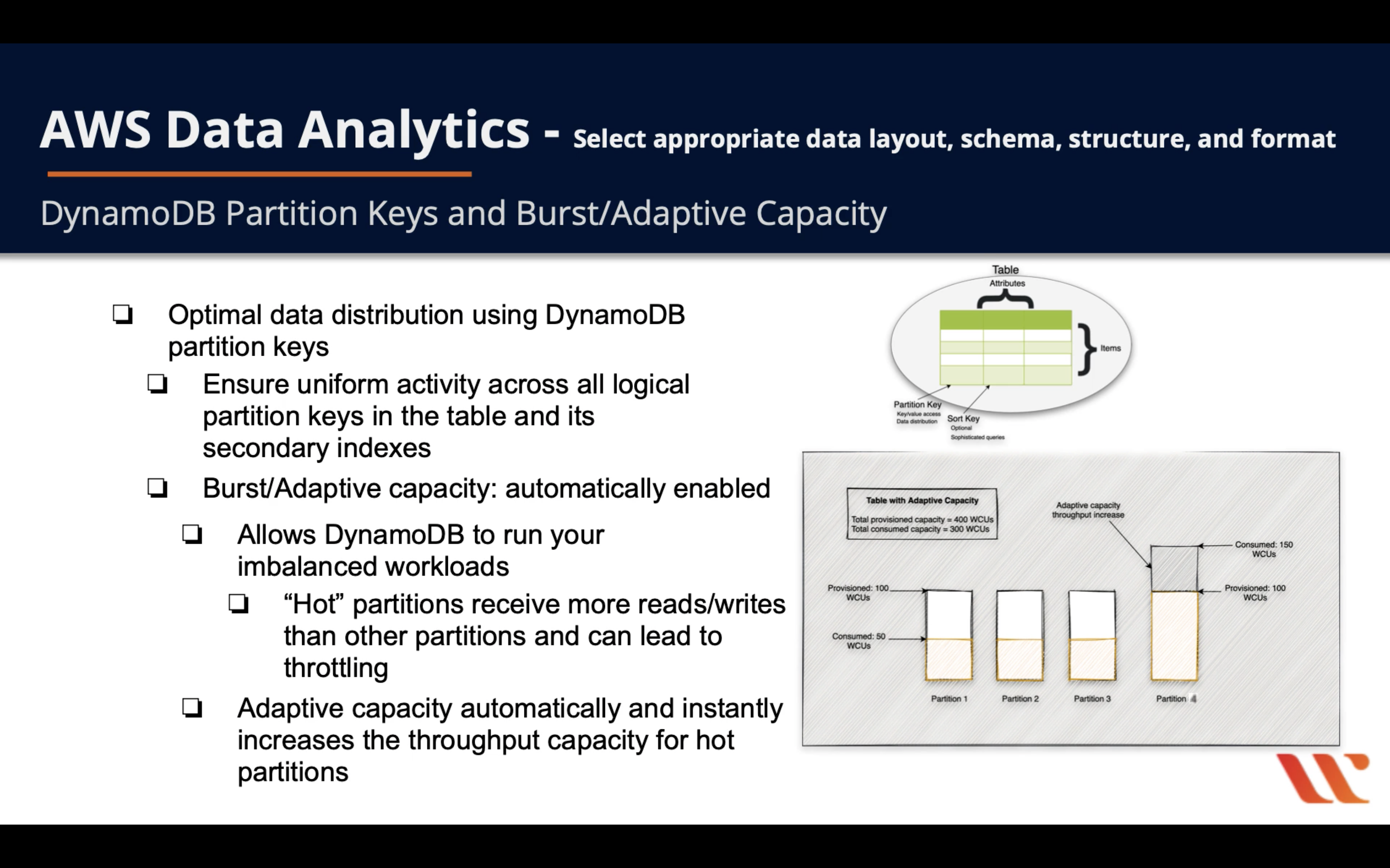
DynamoDB Partition Keys and Burst/Adaptive Capacity
- Optimal data distribution using DynamoDB partition keys
- Ensure uniform activity across all logical partition keys in the table and its secondary indexes
- Burst/Adaptive capacity: automatically enabled
- Allow DynamoDB to run your imbalanced workloads
- “Hot” partitions receive more reads/writes than other partitions and can lead to throttling
- Adaptive capacity automatically and instantly increases the throughput capacity for hot partitions
- Whenever you are not fully using your partition’s throughput, DynamoDB reserves a portion of that unused capacity for Burst capacity
- Allow DynamoDB to run your imbalanced workloads
For example, a DynamoDB contains student_id, student_name, student_gender, and student_gpa.
If student_id is the primary key, obviously student_name have a higher read request and student_gpa has both higher read/write request.
Choosing the Right DynamoDB Partition Key
Recommendations for partition keys
- Use high-cardinality attributes. These are attributes that have distinct values for each item, like
e-mailid,employee_no,customerid,sessionid,orderid, and so on. - Use composite attributes. Try to combine more than one attribute to form a unique key, if that meets your access pattern. For example, consider an orders table with
customerid+productid+countrycodeas the partition key andorder_dateas the sort key. - Cache the popular items when there is a high volume of read traffic using Amazon DynamoDB Accelerator (DAX). The cache acts as a low-pass filter, preventing reads of unusually popular items from swamping partitions. For example, consider a table that has deals information for products. Some deals are expected to be more popular than others during major sale events like Black Friday or Cyber Monday. DAX is a fully managed, in-memory cache for DynamoDB that doesn’t require developers to manage cache invalidation, data population, or cluster management. DAX also is compatible with DynamoDB API calls, so developers can incorporate it more easily into existing applications.
- Add random numbers or digits from a predetermined range for write-heavy use cases. Suppose that you expect a large volume of writes for a partition key (for example, greater than 1000 1 K writes per second). In this case, use an additional prefix or suffix (a fixed number from predetermined range, say 1–10) and add it to the partition key.
For example, consider a table of invoice transactions. A single invoice can contain thousands of transactions per client. How do we enforce uniqueness and ability to query and update the invoice details for high-volumetric clients?
Following is the recommended table layout for this scenario:
- Partition key: Add a random suffix (1–10 or 1–100) with the
InvoiceNumber, depending on the number of transactions perInvoiceNumber. For example, assume that a singleInvoiceNumbercontains up to 50,000 1K items and that you expect 5000 writes per second. In this case, you can use the following formula to estimate the suffix range: (Number of writes per second * (roundup (item size in KB),0)* 1KB ) /1000). Using this formula requires a minimum of five partitions to distribute writes, and hence you might want to set the range as 1-5. - Sort key:
ClientTransactionid
| Partition Key | Sort Key | Attribute1 |
|---|---|---|
| InvoiceNumber+Randomsuffix | ClientTransactionid | Invoice_Date |
| 121212-1 | Client1_trans1 | 2016-05-17 01.36.45 |
| 121212-1 | Client1-trans2 | 2016-05-18 01.36.30 |
| 121212-2 | Client2_trans1 | 2016-06-15 01.36.20 |
| 121212-2 | Client2_trans2 | 2016-07-1 01.36.15 |
- This combination gives us a good spread through the partitions. You can use the sort key to filter for a specific client (for example, where
InvoiceNumber=121212-1andClientTransactionidbegins withClient1). - Because we have a random number appended to our partition key (1–5), we need to query the table five times for a given
InvoiceNumber. Our partition key could be 121212-[1-5], so we need to query where partition key is 121212-1 andClientTransactionidbegins_with Client1. We need to repeat this for 121212-2, on up to 121212-5 and then merge the results.
Performance
Read/Write Capacity Mode
Read/Write Capacity Mode
Amazon DynamoDB pricing
Cost savings with DynamoDB On-Demand: Lessons learned
Amazon DynamoDB has two read/write capacity modes for processing reads and writes on your tables:
- On-demand
- Provisioned (default, free-tier eligible)
The read/write capacity mode controls how you are charged for read and write throughput and how you manage capacity. You can set the read/write capacity mode when creating a table or you can change it later.
Local secondary indexes inherit the read/write capacity mode from the base table. For more information, see Considerations When Changing Read/Write Capacity Mode.
Economics
There are cases where on-demand is significantly more expensive compared to provisioned with Auto Scaling. My rule of thumb: The spikier your workload, the higher the savings with on-demand. Workloads with zero requests also benefit. The reason why we saw such significant savings with marbot is our workload that goes down to almost zero requests/second for half of the day in production and is mostly zero for 24/7 in our test environment. My suggestion is to switch to on-demand for one day and compare your costs with the day before.
With Auto scaling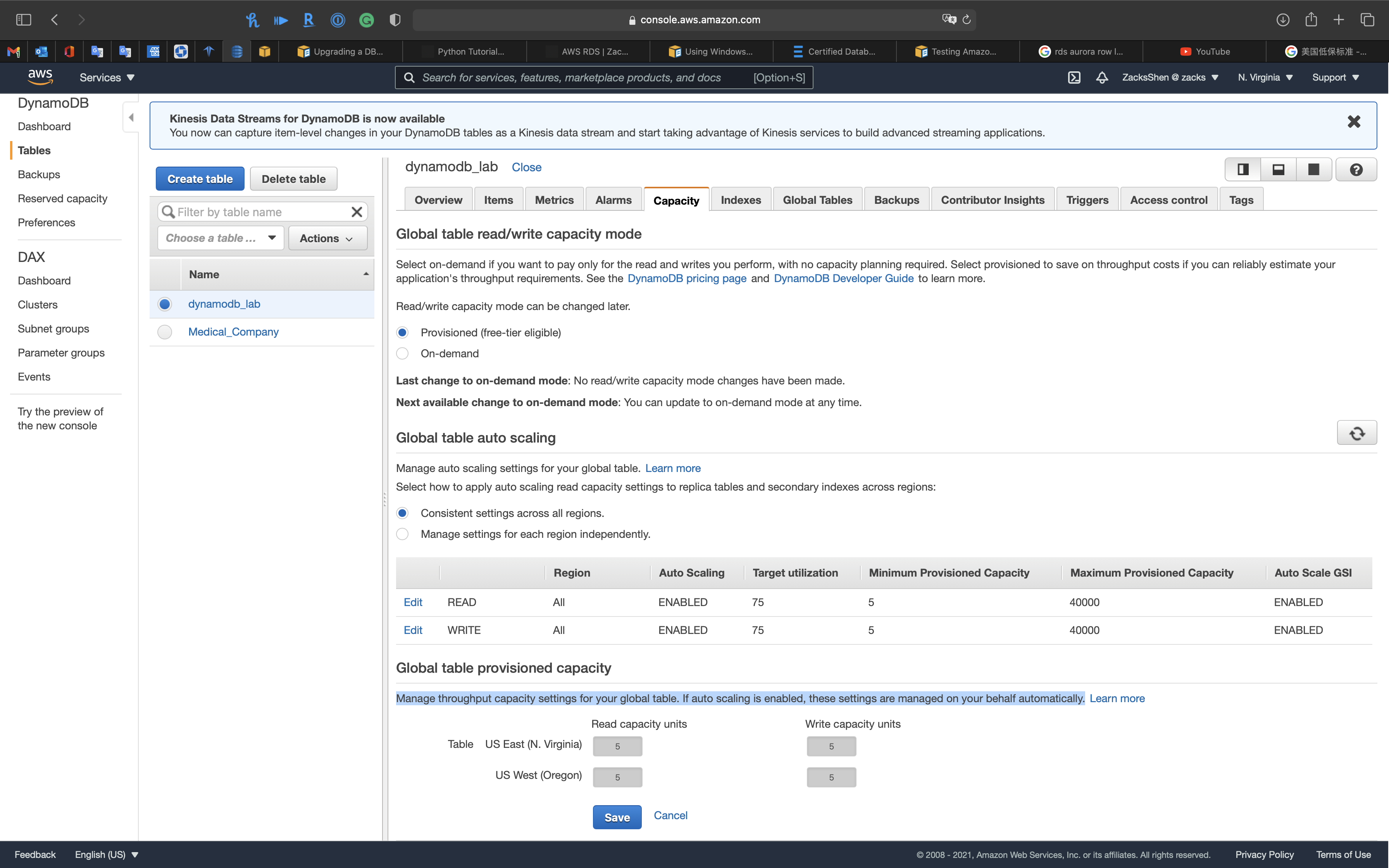
Without Auto scaling: you can customize read/write capacity for each table manually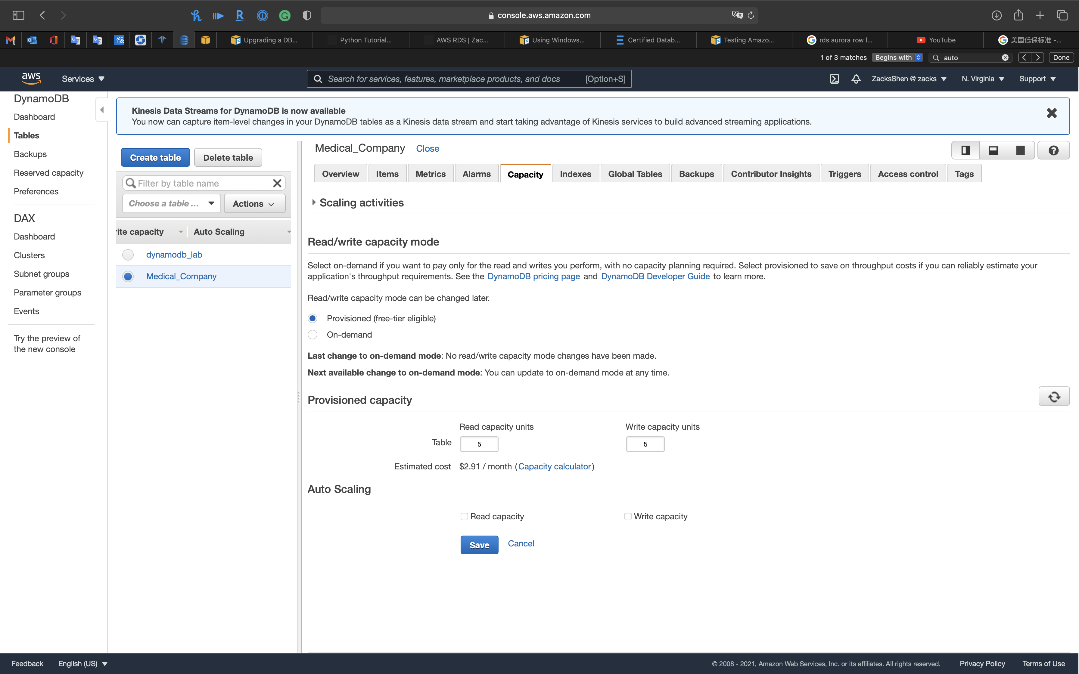
On-Demand Mode
Amazon DynamoDB on-demand is a flexible billing option capable of serving thousands of requests per second without capacity planning. DynamoDB on-demand offers pay-per-request pricing for read and write requests so that you pay only for what you use.
When you choose on-demand mode, DynamoDB instantly accommodates your workloads as they ramp up or down to any previously reached traffic level. If a workload’s traffic level hits a new peak, DynamoDB adapts rapidly to accommodate the workload. Tables that use on-demand mode deliver the same single-digit millisecond latency, service-level agreement (SLA) commitment, and security that DynamoDB already offers. You can choose on-demand for both new and existing tables and you can continue using the existing DynamoDB APIs without changing code.
On-demand mode is a good option if any of the following are true:
- You create new tables with unknown workloads.
- You have unpredictable application traffic.
- You prefer the ease of paying for only what you use.
With on-demand capacity mode, DynamoDB charges you for the data reads and writes your application performs on your tables. You do not need to specify how much read and write throughput you expect your application to perform because DynamoDB instantly accommodates your workloads as they ramp up or down.
Provisioned Mode
If you choose provisioned mode, you specify the number of reads and writes per second that you require for your application. You can use auto scaling to adjust your table’s provisioned capacity automatically in response to traffic changes. This helps you govern your DynamoDB use to stay at or below a defined request rate in order to obtain cost predictability.
Provisioned mode is a good option if any of the following are true:
- You have predictable application traffic.
- You run applications whose traffic is consistent or ramps gradually.
- You can forecast capacity requirements to control costs.
With provisioned capacity mode, you specify the number of reads and writes per second that you expect your application to require. You can use auto scaling to automatically adjust your table’s capacity based on the specified utilization rate to ensure application performance while reducing costs.
DynamoDB Auto Scaling
DynamoDB auto scaling actively manages throughput capacity for tables and global secondary indexes. With auto scaling, you define a range (upper and lower limits) for read and write capacity units. You also define a target utilization percentage within that range. DynamoDB auto scaling seeks to maintain your target utilization, even as your application workload increases or decreases.
With DynamoDB auto scaling, a table or a global secondary index can increase its provisioned read and write capacity to handle sudden increases in traffic, without request throttling. When the workload decreases, DynamoDB auto scaling can decrease the throughput so that you don’t pay for unused provisioned capacity.
Manageability
TTL
Amazon DynamoDB Time to Live (TTL) allows you to define a per-item timestamp to determine when an item is no longer needed. Shortly after the date and time of the specified timestamp, DynamoDB deletes the item from your table without consuming any write throughput. TTL is provided at no extra cost as a means to reduce stored data volumes by retaining only the items that remain current for your workload’s needs.
TTL is useful if you store items that lose relevance after a specific time. The following are example TTL use cases:
- Remove user or sensor data after one year of inactivity in an application.
- Archive expired items to an Amazon S3 data lake via DynamoDB Streams and AWS Lambda.
- Retain sensitive data for a certain amount of time according to contractual or regulatory obligations.
Security
Access Control
Encryption
Availability and Durability
DynamoDB Backups
On-Demand Backup and Restore for DynamoDB
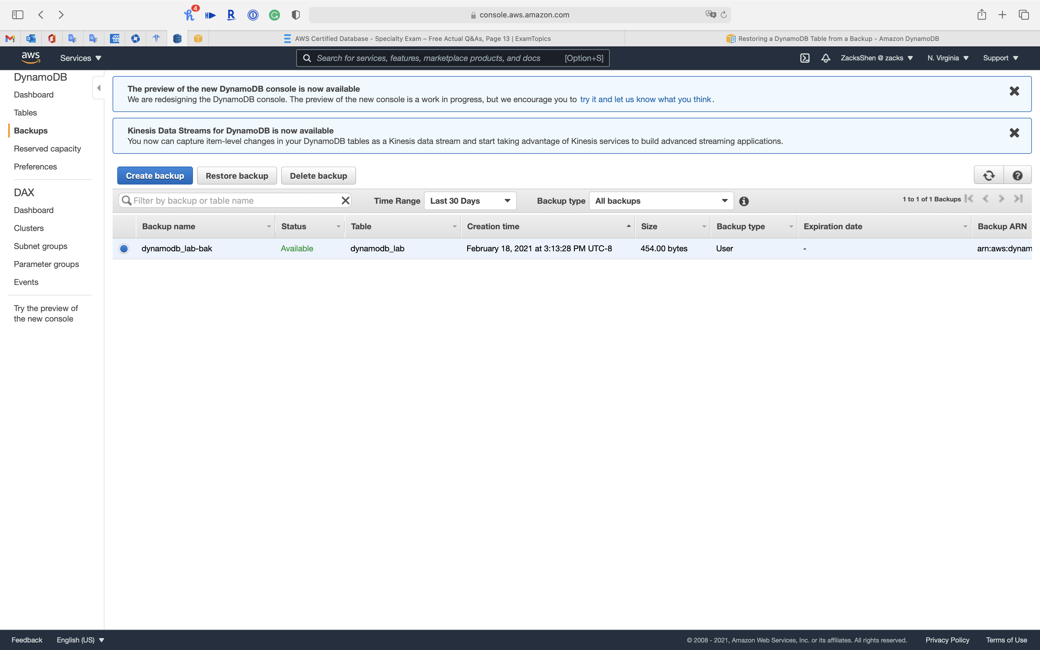
You can create on-demand backups for your Amazon DynamoDB tables or enable continuous backups with point-in-time recovery.
You can use the DynamoDB on-demand backup capability to create full backups of your tables for long-term retention and archival for regulatory compliance needs. You can back up and restore your table data anytime with a single click on the AWS Management Console or with a single API call. Backup and restore actions run with zero impact on table performance or availability.
The on-demand backup and restore process scales without degrading the performance or availability of your applications. It uses a new and unique distributed technology that lets you complete backups in seconds regardless of table size. You can create backups that are consistent within seconds across thousands of partitions without worrying about schedules or long-running backup processes. All on-demand backups are cataloged, discoverable, and retained until explicitly deleted.
In addition, on-demand backup and restore operations don’t affect performance or API latencies. Backups are preserved regardless of table deletion.
Back Up and Restore DynamoDB Tables: How It Works
You can use the on-demand backup feature to create full backups of your Amazon DynamoDB tables. This section provides an overview of what happens during the backup and restore process.
You can schedule periodic or future backups by using AWS Lambda functions.
Backing Up a DynamoDB Table
Backup a DynamoDB Table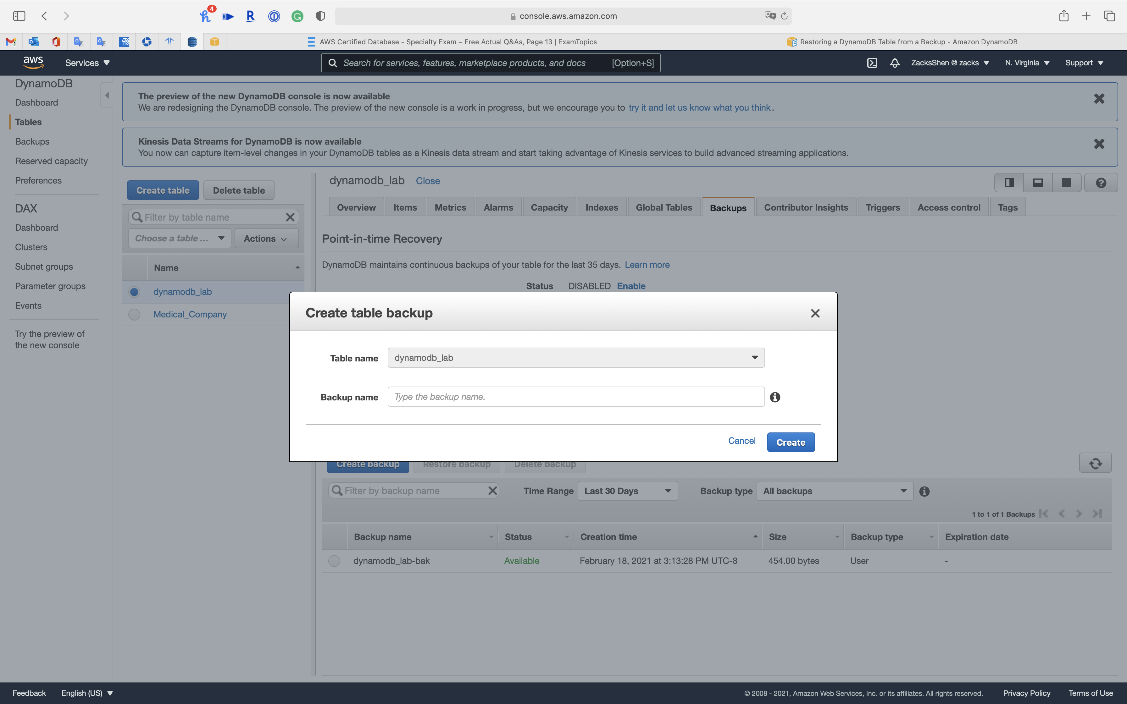
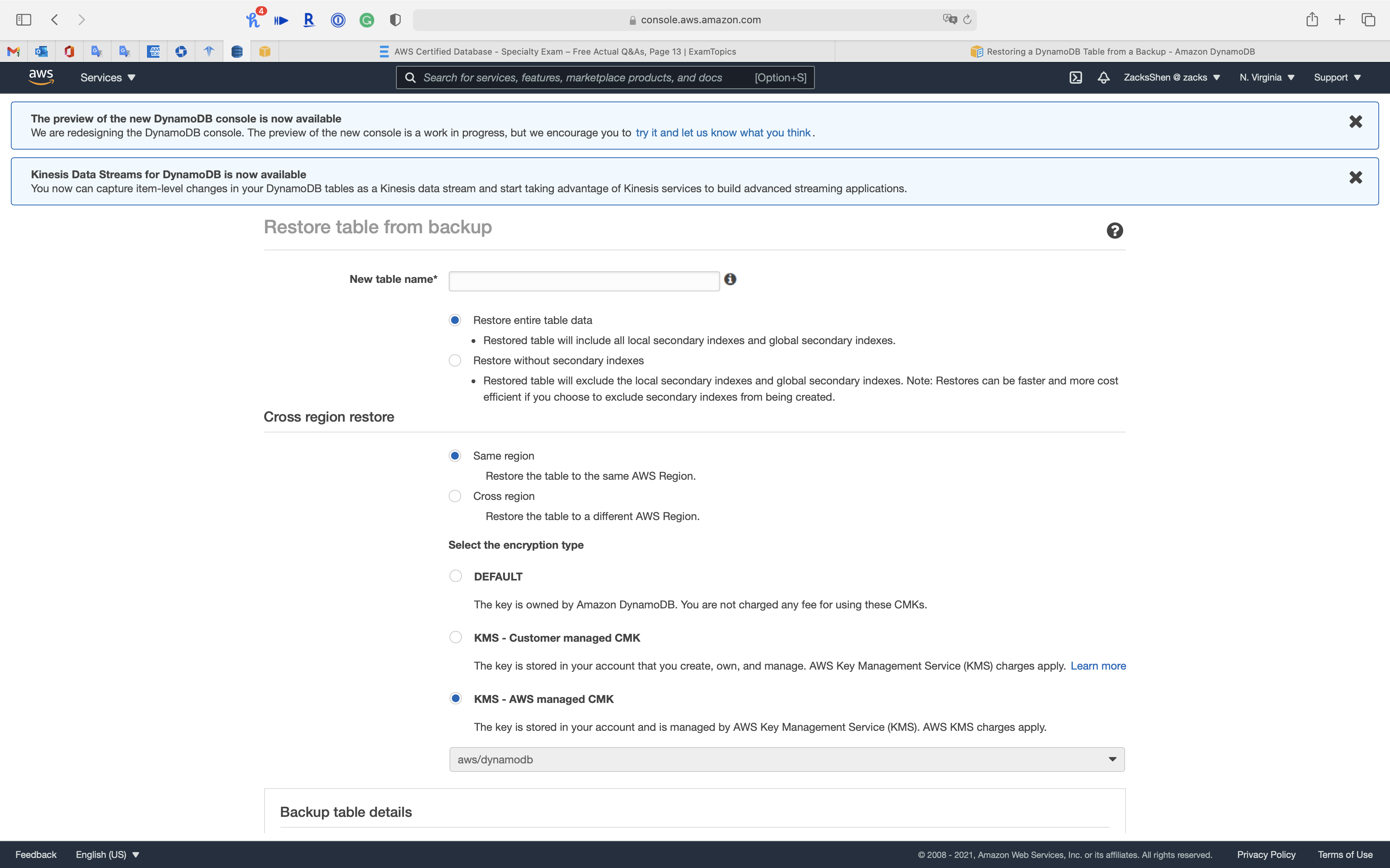
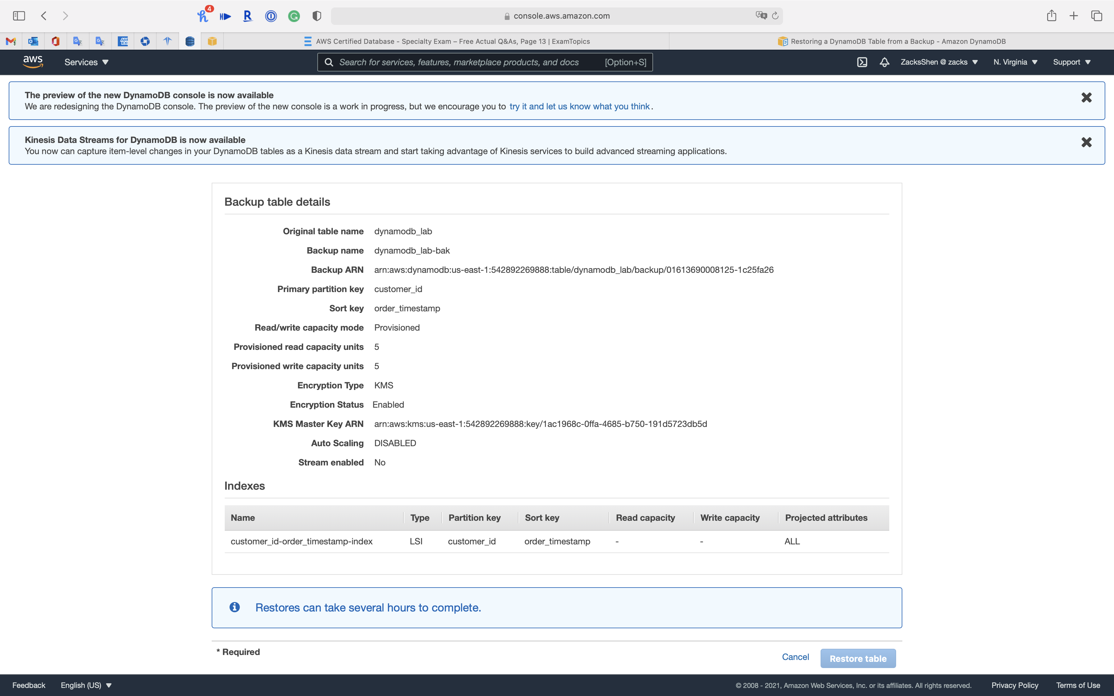
Restoring a DynamoDB Table from a Backup
This section describes how to restore a table from a backup using the Amazon DynamoDB console or the AWS Command Line Interface (AWS CLI).
Deleting a DynamoDB Table Backup
Using IAM with DynamoDB Backup and Restore
Point-in-Time Recovery for DynamoDB
You can create on-demand backups for your Amazon DynamoDB tables or enable continuous backups with point-in-time recovery.
Multi-AZs
A global company wants to run an application in several AWS Regions to support a global user base. The application will need a database that can support a high volume of low-latency reads and writes that is expected to vary over time. The data must be shared across all of the Regions to support dynamic company-wide reports.
Amazon DynamoDB global tables provide a multi-Region, multi-master database in the AWS Regions you specify. DynamoDB performs all of the necessary tasks to create identical tables in these Regions and propagate ongoing data changes to all of them. DynamoDB auto scaling cost effectively adjusts provisioned throughput to actual traffic patterns.
Read Replica
Diaster Recovery
RTO & RPO
Disaster Recovery (DR) Objectives
Plan for Disaster Recovery (DR)
Implementing a disaster recovery strategy with Amazon RDS
| Feature | RTO | RPO | Cost | Scope |
|---|---|---|---|---|
| Automated backups(once a day) | Good | Better | Low | Single Region |
| Manual snapshots | Better | Good | Medium | Cross-Region |
| Read replicas | Best | Best | High | Cross-Region |
In addition to availability objectives, your resiliency strategy should also include Disaster Recovery (DR) objectives based on strategies to recover your workload in case of a disaster event. Disaster Recovery focuses on one-time recovery objectives in response natural disasters, large-scale technical failures, or human threats such as attack or error. This is different than availability which measures mean resiliency over a period of time in response to component failures, load spikes, or software bugs.
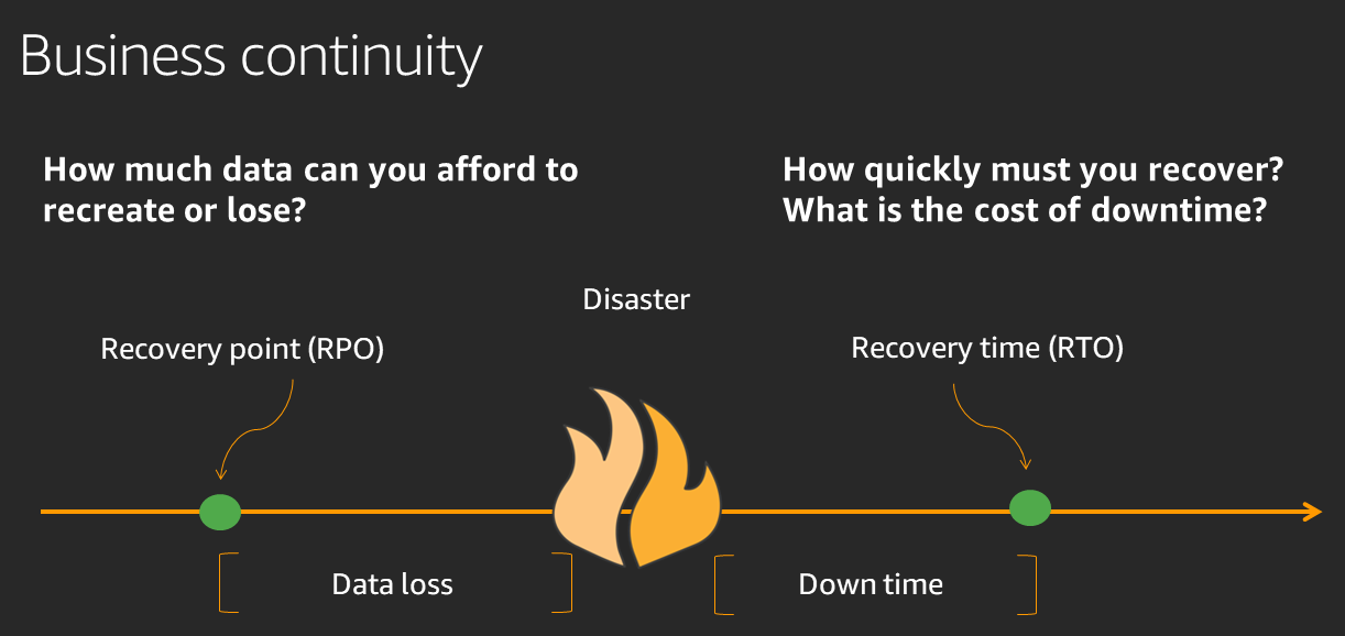
Define recovery objectives for downtime and data loss: The workload has a recovery time objective (RTO) and recovery point objective (RPO).
- Recovery Time Objective (RTO) is defined by the organization. RTO is the maximum acceptable delay between the interruption of service and restoration of service. This determines what is considered an acceptable time window when service is unavailable.
- Recovery Point Objective (RPO) is defined by the organization. RPO is the maximum acceptable amount of time since the last data recovery point. This determines what is considered an acceptable loss of data between the last recovery point and the interruption of service.
Recovery Strategies
Use defined recovery strategies to meet the recovery objectives: A disaster recovery (DR) strategy has been defined to meet objectives. Choose a strategy such as: backup and restore, active/passive (pilot light or warm standby), or active/active.
When architecting a multi-region disaster recovery strategy for your workload, you should choose one of the following multi-region strategies. They are listed in increasing order of complexity, and decreasing order of RTO and RPO. DR Region refers to an AWS Region other than the one primary used for your workload (or any AWS Region if your workload is on premises).
- Backup and restore (RPO in hours, RTO in 24 hours or less): Back up your data and applications using point-in-time backups into the DR Region. Restore this data when necessary to recover from a disaster.
- Pilot light (RPO in minutes, RTO in hours): Replicate your data from one region to another and provision a copy of your core workload infrastructure. Resources required to support data replication and backup such as databases and object storage are always on. Other elements such as application servers are loaded with application code and configurations, but are switched off and are only used during testing or when Disaster Recovery failover is invoked.
- Warm standby (RPO in seconds, RTO in minutes): Maintain a scaled-down but fully functional version of your workload always running in the DR Region. Business-critical systems are fully duplicated and are always on, but with a scaled down fleet. When the time comes for recovery, the system is scaled up quickly to handle the production load. The more scaled-up the Warm Standby is, the lower RTO and control plane reliance will be. When scaled up to full scale this is known as a Hot Standby.
- Multi-region (multi-site) active-active (RPO near zero, RTO potentially zero): Your workload is deployed to, and actively serving traffic from, multiple AWS Regions. This strategy requires you to synchronize data across Regions. Possible conflicts caused by writes to the same record in two different regional replicas must be avoided or handled. Data replication is useful for data synchronization and will protect you against some types of disaster, but it will not protect you against data corruption or destruction unless your solution also includes options for point-in-time recovery. Use services like Amazon Route 53 or AWS Global Accelerator to route your user traffic to where your workload is healthy. For more details on AWS services you can use for active-active architectures see the AWS Regions section of Use Fault Isolation to Protect Your Workload.
Recommendation
The difference between Pilot Light and Warm Standby can sometimes be difficult to understand. Both include an environment in your DR Region with copies of your primary region assets. The distinction is that Pilot Light cannot process requests without additional action taken first, while Warm Standby can handle traffic (at reduced capacity levels) immediately. Pilot Light will require you to turn on servers, possibly deploy additional (non-core) infrastructure, and scale up, while Warm Standby only requires you to scale up (everything is already deployed and running). Choose between these based on your RTO and RPO needs.
Tips
Test disaster recovery implementation to validate the implementation: Regularly test failover to DR to ensure that RTO and RPO are met.
A pattern to avoid is developing recovery paths that are rarely executed. For example, you might have a secondary data store that is used for read-only queries. When you write to a data store and the primary fails, you might want to fail over to the secondary data store. If you don’t frequently test this failover, you might find that your assumptions about the capabilities of the secondary data store are incorrect. The capacity of the secondary, which might have been sufficient when you last tested, may be no longer be able to tolerate the load under this scenario. Our experience has shown that the only error recovery that works is the path you test frequently. This is why having a small number of recovery paths is best. You can establish recovery patterns and regularly test them. If you have a complex or critical recovery path, you still need to regularly execute that failure in production to convince yourself that the recovery path works. In the example we just discussed, you should fail over to the standby regularly, regardless of need.
Manage configuration drift at the DR site or region: Ensure that your infrastructure, data, and configuration are as needed at the DR site or region. For example, check that AMIs and service quotas are up to date.
AWS Config continuously monitors and records your AWS resource configurations. It can detect drift and trigger AWS Systems Manager Automation to fix it and raise alarms. AWS CloudFormation can additionally detect drift in stacks you have deployed.
Automate recovery: Use AWS or third-party tools to automate system recovery and route traffic to the DR site or region.
Based on configured health checks, AWS services, such as Elastic Load Balancing and AWS Auto Scaling, can distribute load to healthy Availability Zones while services, such as Amazon Route 53 and AWS Global Accelerator, can route load to healthy AWS Regions.
For workloads on existing physical or virtual data centers or private clouds CloudEndure Disaster Recovery, available through AWS Marketplace, enables organizations to set up an automated disaster recovery strategy to AWS. CloudEndure also supports cross-region / cross-AZ disaster recovery in AWS.
Migration
Monitoring
Logging and Monitoring
Amazon DocumentDB (with MongoDB compatibility) provides a variety of Amazon CloudWatch metrics that you can monitor to determine the health and performance of your Amazon DocumentDB clusters and instances. You can view Amazon DocumentDB metrics using various tools, including the Amazon DocumentDB console, the AWS CLI, the Amazon CloudWatch console, and the CloudWatch API. For more information about monitoring, see Monitoring Amazon DocumentDB.
In addition to Amazon CloudWatch metrics, you can use the profiler to log the execution time and details of operations that were performed on your cluster. Profiler is useful for monitoring the slowest operations on your cluster to help you improve individual query performance and overall cluster performance. When enabled, operations are logged to Amazon CloudWatch Logs and you can use CloudWatch Insight to analyze, monitor, and archive your Amazon DocumentDB profiling data. For more information, see Profiling Amazon DocumentDB Operations.
Amazon DocumentDB also integrates with AWS CloudTrail, a a service that provides a record of actions taken by IAM users, IAM roles, or an AWS service in Amazon DocumentDB (with MongoDB compatibility). CloudTrail captures all AWS CLI API calls for Amazon DocumentDB as events, including calls from the Amazon DocumentDB AWS Management Console and from code calls to the Amazon DocumentDB SDK. For more information, see Logging Amazon DocumentDB API Calls with AWS CloudTrail.
With Amazon DocumentDB, you can audit events that were performed in your cluster. Examples of logged events include successful and failed authentication attempts, dropping a collection in a database, or creating an index. By default, auditing is disabled on Amazon DocumentDB and requires that you opt in to this feature. For more information, see Auditing Amazon DocumentDB Events.
Auditing Amazon DocumentDB Events
With Amazon DocumentDB (with MongoDB compatibility), you can audit events that were performed in your cluster. Examples of logged events include successful and failed authentication attempts, dropping a collection in a database, or creating an index. By default, auditing is disabled on Amazon DocumentDB and requires that you opt in to use this feature.
When auditing is enabled, Amazon DocumentDB records Data Definition Language (DDL), authentication, authorization, and user management events to Amazon CloudWatch Logs. When auditing is enabled, Amazon DocumentDB exports your cluster’s auditing records (JSON documents) to Amazon CloudWatch Logs. You can use Amazon CloudWatch Logs to analyze, monitor, and archive your Amazon DocumentDB auditing events.
Amazon DynamoDB Accelerator (DAX)
Amazon DynamoDB Accelerator (DAX) is a fully managed, highly available, in-memory cache for Amazon DynamoDB that delivers up to a 10 times performance improvement—from milliseconds to microseconds—even at millions of requests per second.
DAX does all the heavy lifting required to add in-memory acceleration to your DynamoDB tables, without requiring developers to manage cache invalidation, data population, or cluster management.
Now you can focus on building great applications for your customers without worrying about performance at scale. You do not need to modify application logic because DAX is compatible with existing DynamoDB API calls. Learn more in the DynamoDB Developer Guide.
You can enable DAX with just a few clicks in the AWS Management Console or by using the AWS SDK. Just as with DynamoDB, you only pay for the capacity you provision. Learn more about DAX pricing on the pricing page.
In-Memory Acceleration with DynamoDB Accelerator (DAX)
Amazon DynamoDB is designed for scale and performance. In most cases, the DynamoDB response times can be measured in single-digit milliseconds. However, there are certain use cases that require response times in microseconds. For these use cases, DynamoDB Accelerator (DAX) delivers fast response times for accessing eventually consistent data.
DAX is a DynamoDB-compatible caching service that enables you to benefit from fast in-memory performance for demanding applications. DAX addresses three core scenarios:
- As an in-memory cache, DAX reduces the response times of eventually consistent read workloads by an order of magnitude from single-digit milliseconds to microseconds.
- DAX reduces operational and application complexity by providing a managed service that is API-compatible with DynamoDB. Therefore, it requires only minimal functional changes to use with an existing application.
- For read-heavy or bursty workloads, DAX provides increased throughput and potential operational cost savings by reducing the need to overprovision read capacity units. This is especially beneficial for applications that require repeated reads for individual keys.
DAX supports server-side encryption. With encryption at rest, the data persisted by DAX on disk will be encrypted. DAX writes data to disk as part of propagating changes from the primary node to read replicas. For more information, see DAX Encryption at Rest.
DAX: How It Works
Amazon DynamoDB Accelerator (DAX) is designed to run within an Amazon Virtual Private Cloud (Amazon VPC) environment. The Amazon VPC service defines a virtual network that closely resembles a traditional data center. With a VPC, you have control over its IP address range, subnets, routing tables, network gateways, and security settings. You can launch a DAX cluster in your virtual network and control access to the cluster by using Amazon VPC security groups.
The following diagram shows a high-level overview of DAX.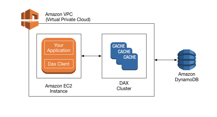
To create a DAX cluster, you use the AWS Management Console. Unless you specify otherwise, your DAX cluster runs within your default VPC. To run your application, you launch an Amazon EC2 instance into your Amazon VPC. You then deploy your application (with the DAX client) on the EC2 instance.
At runtime, the DAX client directs all of your application’s DynamoDB API requests to the DAX cluster. If DAX can process one of these API requests directly, it does so. Otherwise, it passes the request through to DynamoDB.
Finally, the DAX cluster returns the results to your application.
Best Practices
Modeling Game Player Data with Amazon DynamoDB
Modeling Game Player Data with Amazon DynamoDB
Amazon DynamoDB: Gaming use cases and design patterns
Choosing the Right DynamoDB Partition Key
| Use case | Design pattern |
|---|---|
| Game state, player data store | 1:1 modeling, 1:M modeling |
| Player session history data store | 1:1 modeling, 1:M modeling |
| Leaderboard | N:M modeling |
Game state, player data store | 1:1 modeling, 1:M modeling
EA uses DynamoDB to store game state, user data, and game inventory data in multiple tables. EA uses the user ID as the partition key and primary key (a 1:1 modeling pattern).
Design patterns: To store data in DynamoDB, gaming companies partition game state and other player data using player ID, and use the key-value access pattern (1:1 modeling). In cases when more fine-grained access is called for, these companies use a sort key (1:M modeling). This allows them to access and update different properties or subsets of a player’s dataset separately. This way, they don’t have to retrieve an entire dataset. In this approach, multiple items that store different properties can be updated transactionally by using the DynamoDB transactional API. Some companies compress user data to reduce cost. PennyPop, for example, uses gzip to compress player data and store it as a base64 string, reducing the player data to 10 percent of its original size.
Player session history data store | 1:1 modeling, 1:M modeling
Design patterns: To store player session history and other time-oriented data in DynamoDB, gaming companies usually use the player ID as the partition key and the date and time, such as last login, as the sort key (1:M modeling). This schema allows these companies to access each player’s data efficiently by using the player ID and date and time. Queries can be easily tailored to select a single record for a specific date and time, or a set of records for a given range of date and time.
Leaderboard | N:M modeling
Design patterns: With a table partitioned by player ID that stores players’ game state, including the top score as an attribute, a leaderboard can be implemented with a global secondary index. The index would use the game ID or name as the partition key, and the top-score attribute as the sort key (N:M modeling). This is described in the Global Secondary Indexes section of the DynamoDB Developer Guide.
Best Practices for Designing and Using Partition Keys Effectively
Best Practices for Designing and Using Partition Keys Effectively
Modify auto scaling for read or write capacity of provisioned table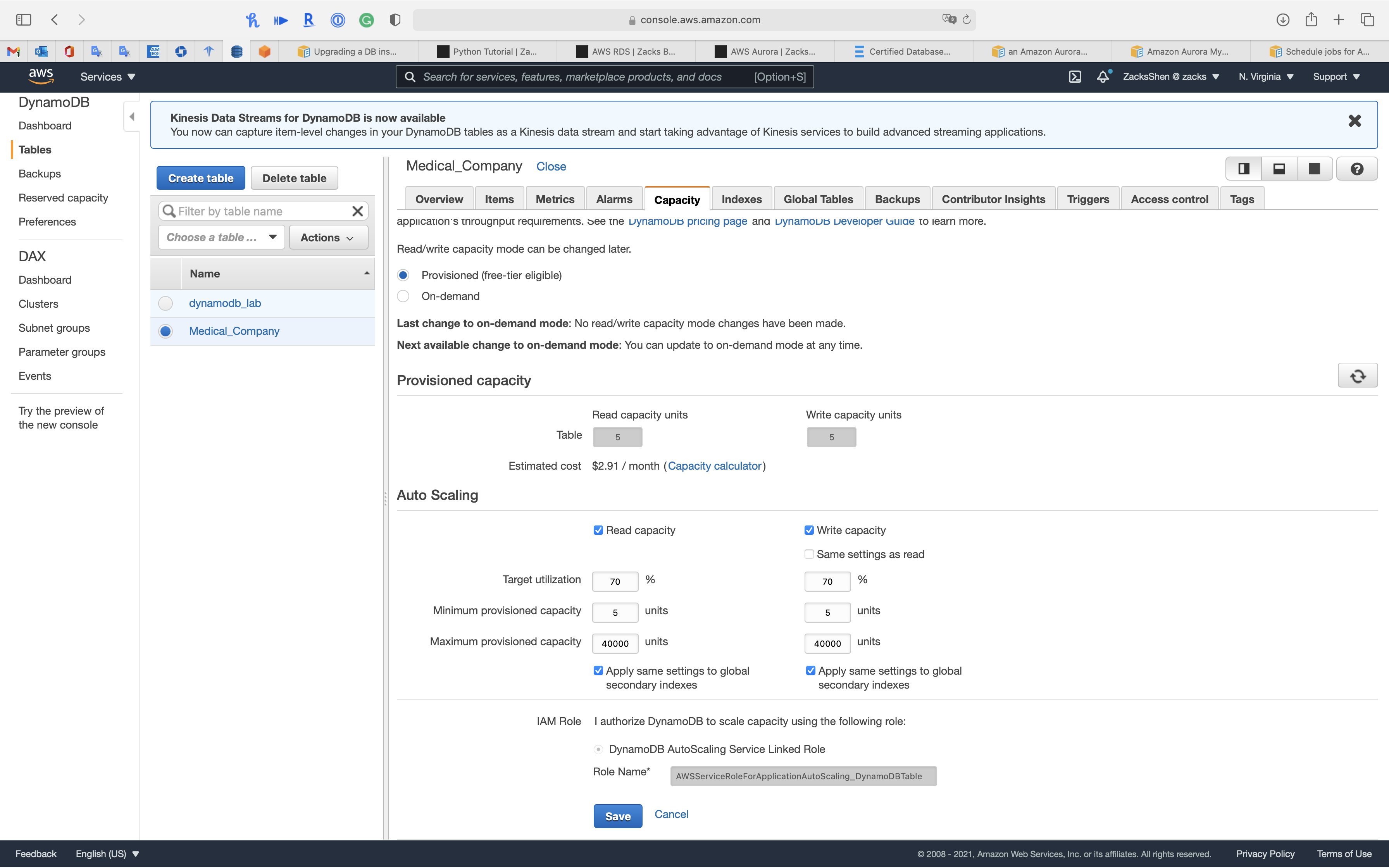
Using Burst Capacity Effectively
DynamoDB provides some flexibility in your per-partition throughput provisioning by providing burst capacity. Whenever you’re not fully using a partition’s throughput, DynamoDB reserves a portion of that unused capacity for later bursts of throughput to handle usage spikes.
DynamoDB currently retains up to 5 minutes (300 seconds) of unused read and write capacity. During an occasional burst of read or write activity, these extra capacity units can be consumed quickly—even faster than the per-second provisioned throughput capacity that you’ve defined for your table.
DynamoDB can also consume burst capacity for background maintenance and other tasks without prior notice.
Note that these burst capacity details might change in the future.
Understanding DynamoDB Adaptive Capacity
Adaptive capacity is a feature that enables DynamoDB to run imbalanced workloads indefinitely. It minimizes throttling due to throughput exceptions. It also helps you reduce costs by enabling you to provision only the throughput capacity that you need.
Adaptive capacity is enabled automatically for every DynamoDB table, at no additional cost. You don’t need to explicitly enable or disable it.
Boost Throughput Capacity to High-Traffic Partitions
It’s not always possible to distribute read and write activity evenly. When data access is imbalanced, a “hot” partition can receive a higher volume of read and write traffic compared to other partitions. In extreme cases, throttling can occur if a single partition receives more than 3,000 RCUs or 1,000 WCUs.
To better accommodate uneven access patterns, DynamoDB adaptive capacity enables your application to continue reading and writing to hot partitions without being throttled, provided that traffic does not exceed your table’s total provisioned capacity or the partition maximum capacity. Adaptive capacity works by automatically and instantly increasing throughput capacity for partitions that receive more traffic.
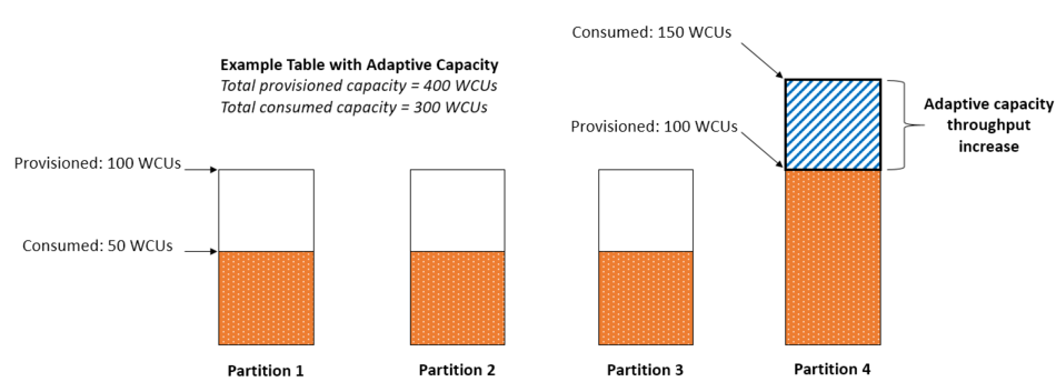
The following diagram illustrates how adaptive capacity works. The example table is provisioned with 400 WCUs evenly shared across four partitions, allowing each partition to sustain up to 100 WCUs per second. Partitions 1, 2, and 3 each receives write traffic of 50 WCU/sec. Partition 4 receives 150 WCU/sec. This hot partition can accept write traffic while it still has unused burst capacity, but eventually it throttles traffic that exceeds 100 WCU/sec.
DynamoDB adaptive capacity responds by increasing partition 4’s capacity so that it can sustain the higher workload of 150 WCU/sec without being throttled.
Isolate Frequently Accessed Items
If your application drives disproportionately high traffic to one or more items, adaptive capacity rebalances your partitions such that frequently accessed items don’t reside on the same partition. This isolation of frequently accessed items reduces the likelihood of request throttling due to your workload exceeding the throughput quota on a single partition.
If your application drives consistently high traffic to a single item, adaptive capacity might rebalance your data such that a partition contains only that single, frequently accessed item. In this case, DynamoDB can deliver throughput up to the partition maximum of 3,000 RCUs or 1,000 WCUs to that single item’s primary key.
Example of Modeling Relational Data in DynamoDB
This example describes how to model relational data in Amazon DynamoDB. A DynamoDB table design corresponds to the relational order entry schema that is shown in Relational Modeling. It follows the Adjacency List Design Pattern, which is a common way to represent relational data structures in DynamoDB.
The design pattern requires you to define a set of entity types that usually correlate to the various tables in the relational schema. Entity items are then added to the table using a compound (partition and sort) primary key. The partition key of these entity items is the attribute that uniquely identifies the item and is referred to generically on all items as PK. The sort key attribute contains an attribute value that you can use for an inverted index or global secondary index. It is generically referred to as SK.
You define the following entities, which support the relational order entry schema.
- HR-Employee - PK: EmployeeID, SK: Employee Name
- HR-Region - PK: RegionID, SK: Region Name
- HR-Country - PK: CountryId, SK: Country Name
- HR-Location - PK: LocationID, SK: Country Name
- HR-Job - PK: JobID, SK: Job Title
- HR-Department - PK: DepartmentID, SK: DepartmentID
- OE-Customer - PK: CustomerID, SK: AccountRepID
- OE-Order - PK OrderID, SK: CustomerID
- OE-Product - PK: ProductID, SK: Product Name
- OE-Warehouse - PK: WarehouseID, SK: Region Name
After adding these entity items to the table, you can define the relationships between them by adding edge items to the entity item partitions. The following table demonstrates this step.
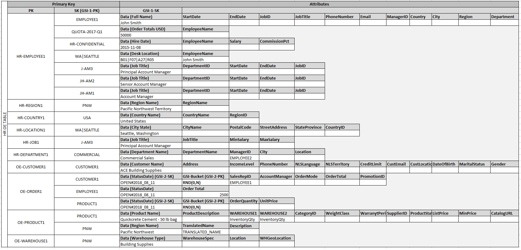
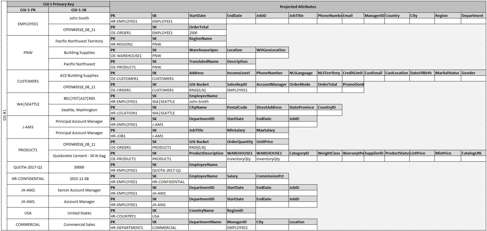
In this example, the Employee, Order, and Product Entity partitions on the table have additional edge items that contain pointers to other entity items on the table. Next, define a few global secondary indexes (GSIs) to support all the access patterns defined previously. The entity items don’t all use the same type of value for the primary key or the sort key attribute. All that is required is to have the primary key and sort key attributes present to be inserted on the table.
The fact that some of these entities use proper names and others use other entity IDs as sort key values allows the same global secondary index to support multiple types of queries. This technique is called GSI overloading. It effectively eliminates the default limit of 20 global secondary indexes for tables that contain multiple item types. This is shown in the following diagram as GSI 1.
GSI 2 is designed to support a fairly common application access pattern, which is to get all the items on the table that have a certain state. For a large table with an uneven distribution of items across available states, this access pattern can result in a hot key, unless the items are distributed across more than one logical partition that can be queried in parallel. This design pattern is called write sharding.
To accomplish this for GSI 2, the application adds the GSI 2 primary key attribute to every Order item. It populates that with a random number in a range of 0–N, where N can generically be calculated using the following formula, unless there is a specific reason to do otherwise.
1 | ItemsPerRCU = 4KB / AvgItemSize |
For example, assume that you expect the following:
- Up to 2 million orders will be in the system, growing to 3 million in 5 years.
- Up to 20 percent of these orders will be in an OPEN state at any given time.
- The average order record is around 100 bytes, with three OrderItem records in the order partition that are around 50 bytes each, giving you an average order entity size of 250 bytes.
For that table, the N factor calculation would look like the following.
1 | ItemsPerRCU = 4KB / 250B = 16 |
In this case, you need to distribute all the orders across at least 13 logical partitions on GSI 2 to ensure that a read of all Order items with an OPEN status doesn’t cause a hot partition on the physical storage layer. It is a good practice to pad this number to allow for anomalies in the dataset. So a model using N = 15 is probably fine. As mentioned earlier, you do this by adding the random 0–N value to the GSI 2 PK attribute of each Order and OrderItem record that is inserted on the table.
This breakdown assumes that the access pattern that requires gathering all OPEN invoices occurs relatively infrequently so that you can use burst capacity to fulfill the request. You can query the following global secondary index using a State and Date Range Sort Key condition to produce a subset or all Orders in a given state as needed.
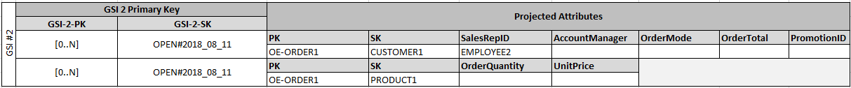
In this example, the items are randomly distributed across the 15 logical partitions. This structure works because the access pattern requires a large number of items to be retrieved. Therefore, it’s unlikely that any of the 15 threads will return empty result sets that could potentially represent wasted capacity. A query always uses 1 read capacity unit (RCU) or 1 write capacity unit (WCU), even if nothing is returned or no data is written.
If the access pattern requires a high velocity query on this global secondary index that returns a sparse result set, it’s probably better to use a hash algorithm to distribute the items rather than a random pattern. In this case, you might select an attribute that is known when the query is run at runtime and hash that attribute into a 0–14 key space when the items are inserted. Then they can be efficiently read from the global secondary index.
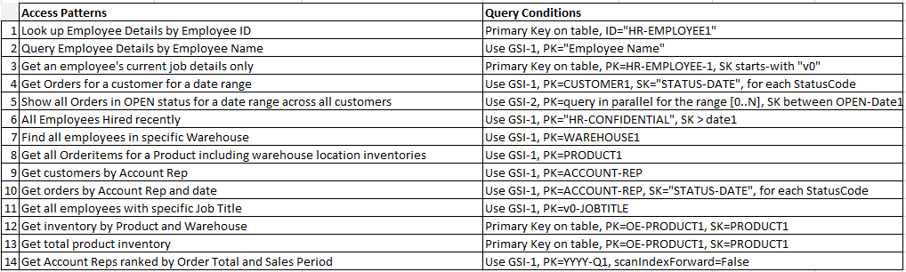
Finally, you can revisit the access patterns that were defined earlier. Following is the list of access patterns and the query conditions that you will use with the new DynamoDB version of the application to accommodate them.