Udacity Software Engineering
Home Page
References
Introduction
Corse Overview
How this Course is Organized
- Software Engineering Practices Part 1 covers how to write well documented, modularized code.
- Software Engineering Practices Part 2 discusses testing your code and logging.
- Introduction to Object-Oriented Programming gives you an overview of this programming style and prepares you to write your own Python package.
- Introduction to Web Development covers building a web application data dashboard.
Course Portfolio Exercises
The software engineering course has two portfolio exercises: building a Python package and developing a web data dashboard. These exercises are NOT reviewed and are NOT required to graduate from the data scientist nanodegree program. In other words, you will not submit either of the portfolio projects to the Udacity review system. Instead, you can use these projects to practice your software engineering skills and then add the projects to your professional portfolio.
Having said that, the skills covered in this course will set you up for success in other Udacity courses with required projects. For example, the data engineering for data scientists course has a required project where you are expected to write clean, concise and well-documented code. You will also have an easier time with that project if you understand the fundamentals of object-oriented programming and a basic understanding of how the backend and frontend of a website works.
Software Engineering Practices, Part I
Introduction
In this lesson, you’ll learn about the following software engineering practices and how they apply in data science.
- Writing clean and modular code
- Writing efficient code
- Code refactoring
- Adding meaningful documentation
- Using version control
In the lesson following this one (part 2), you’ll also learn about the following software engineering practices:
- Testing
- Logging
- Code reviews
Clean and Modular Code
- Production code: Software running on production servers to handle live users and data of the intended audience. Note that this is different from production-quality code, which describes code that meets expectations for production in reliability, efficiency, and other aspects. Ideally, all code in production meets these expectations, but this is not always the case.
- Clean code: Code that is readable, simple, and concise. Clean production-quality code is crucial for collaboration and maintainability in software development.
- Modular code: Code that is logically broken up into functions and modules. Modular production-quality code that makes your code more organized, efficient, and reusable.
- Module: A file. Modules allow code to be reused by encapsulating them into files that can be imported into other files.
Which of the following describes code that is clean? Select all the answers that apply.
Repetitive
Simple
Readable
Vague
Concise
Making your code modular makes it easier to do which of the following things? There may be more than one correct answer.
Reuse your code
Write less code
Read your code
Collaborate your code
Refactoring Code
Refactoring Code
- Refactoring: Restructuring your code to improve its internal structure without changing its external functionality. This gives you a chance to clean and modularize your program after you’ve got it working.
- Since it isn’t easy to write your best code while you’re still trying to just get it working, allocating time to do this is essential to producing high-quality code. Despite the initial time and effort required, this really pays off by speeding up your development time in the long run.
- You become a much stronger programmer when you’re constantly looking to improve your code. The more you refactor, the easier it will be to structure and write good code the first time.
Writing Clean Code
Writing clean code: Meaningful names
Use meaningful names
- Be descriptive and imply type: For booleans, you can prefix with
is_orhas_to make it clear it is a condition. You can also use parts of speech to imply types, like using verbs for functions and nouns for variables. - Be consistent but clearly differentiate:
age_listandageis easier to differentiate thanagesandage. - Avoid abbreviations and single letters: You can determine when to make these exceptions based on the audience for your code. If you work with other data scientists, certain variables may be common knowledge. While if you work with full stack engineers, it might be necessary to provide more descriptive names in these cases as well. (Exceptions include counters and common math variables.)
- Long names aren’t the same as descriptive names: You should be descriptive, but only with relevant information. For example, good function names describe what they do well without including details about implementation or highly specific uses.
Try testing how effective your names are by asking a fellow programmer to guess the purpose of a function or variable based on its name, without looking at your code. Coming up with meaningful names often requires effort to get right.
Writing clean code: Nice whitespace
Use whitespace properly.
- Organize your code with consistent indentation: the standard is to use four spaces for each indent. You can make this a default in your text editor.
- Separate sections with blank lines to keep your code well organized and readable.
- Try to limit your lines to around 79 characters, which is the guideline given in the PEP 8 style guide. In many good text editors, there is a setting to display a subtle line that indicates where the 79 character limit is.
For more guidelines, check out the code layout section of PEP 8 in the following notes.
References
Quiz: Clean Code
Quiz: Categorizing tasks
Imagine you are writing a program that executes a number of tasks and categorizes each task based on its execution time. Below is a small snippet of this program. Which of the following naming changes could make this code cleaner? There may be more than one correct answer.
1 | t = end_time - start # compute execution time |
None
Rename the variable start to start_time to make it consistent with end_time
Rename the variable t to execution_time to make it more descriptive.
Rename the function category to categorize_task to math the part of speech.
Rename the variable c to category to make it more descriptive.
Quiz: Buying stocks
Imagine you analyzed several stocks and calculated the ideal price, or limit price, at which you’d want to buy each stock. You write a program to iterate through your stocks and buy it if the current price is below or equal to the limit price you computed. Otherwise, you put it on a watchlist. Below are three ways of writing this code. Which of the following is the most clean?
1 | # Choice A |
Choice A
Choice B
Choice C
Writing Modular Code
Writing Modular Code
Follow the tips below to write modular code.
Tip: DRY (Don’t Repeat Yourself)
Don’t repeat yourself! Modularization allows you to reuse parts of your code. Generalize and consolidate repeated code in functions or loops.
Tip: Abstract out logic to improve readability
Abstracting out code into a function not only makes it less repetitive, but also improves readability with descriptive function names. Although your code can become more readable when you abstract out logic into functions, it is possible to over-engineer this and have way too many modules, so use your judgement.
Tip: Minimize the number of entities (functions, classes, modules, etc.)
There are trade-offs to having function calls instead of inline logic. If you have broken up your code into an unnecessary amount of functions and modules, you’ll have to jump around everywhere if you want to view the implementation details for something that may be too small to be worth it. Creating more modules doesn’t necessarily result in effective modularization.
Tip: Functions should do one thing
Each function you write should be focused on doing one thing. If a function is doing multiple things, it becomes more difficult to generalize and reuse. Generally, if there’s an “and” in your function name, consider refactoring.
Tip: Arbitrary variable names can be more effective in certain functions
Arbitrary variable names in general functions can actually make the code more readable.
Tip: Try to use fewer than three arguments per function
Try to use no more than three arguments when possible. This is not a hard rule and there are times when it is more appropriate to use many parameters. But in many cases, it’s more effective to use fewer arguments. Remember we are modularizing to simplify our code and make it more efficient. If your function has a lot of parameters, you may want to rethink how you are splitting this up.
Exercise: Refactoring - Wine quality
In this exercise, you’ll refactor code that analyzes a wine quality dataset taken from the UCI Machine Learning Repository. Each row contains data on a wine sample, including several physicochemical properties gathered from tests, as well as a quality rating evaluated by wine experts.
Download the notebook file refactor_wine_quality.ipynb and the dataset winequality-red.csv. Open the notebook file using the Jupyter Notebook. Follow the instructions in the notebook to complete the exercise.
Supporting Materials
Solution: Refactoring – Wine quality
The following code shows the solution code. You can download the solution notebook file that contains the solution code.
1 | import pandas as pd |
My solution.
1 | import pandas as pd |
Supporting Materials
Efficient Code
Efficient Code
Knowing how to write code that runs efficiently is another essential skill in software development. Optimizing code to be more efficient can mean making it:
- Execute faster
- Take up less space in memory/storage
The project on which you’re working determines which of these is more important to optimize for your company or product. When you’re performing lots of different transformations on large
Optimizing - Common Books
Resources:
Exercise: Optimizing – Common books
We provide the code your coworker wrote to find the common book IDs in books_published_last_two_years.txt and all_coding_books.txt to obtain a list of recent coding books. Can you optimize it?
Download the notebook file optimizing_code_common_books.ipynb and the text files. Open the notebook file using the Jupyter Notebook. Follow the instructions in the notebook to complete the exercise.
You can also take a look at the example notebook optimizing_code_common_books_example.ipynb to help you finish the exercise.
Supporting Materials
- All Coding Books
- Books Published Last Two Years
- Optimizing Code Common Books
- Optimizing Code Common Books Example
Solution: Optimizing - Common books
The following code shows the solution code. You can download the solution notebook file that contains the solution code.
1 | import time |
Supporting Materials
Exercise: Optimizing - Holiday Gifts
In the last example, you learned that using vectorized operations and more efficient data structures can optimize your code. Let’s use these tips for one more exercise.
Your online gift store has one million users that each listed a gift on a wishlist. You have the prices for each of these gifts stored in gift_costs.txt. For the holidays, you’re going to give each customer their wishlist gift for free if the cost is under $25. Now, you want to calculate the total cost of all gifts under $25 to see how much you’d spend on free gifts.
Download the notebook file optimizing_code_holiday_gifts.ipynb and the gift_costs.txt file. Open the notebook file using the Jupyter Notebook. Follow the instructions in the notebook to complete the exercise.
Supporting Materials
Solution: Optimizing – Holiday gifts
The following code shows the solution code. You can download the solution notebook file that contains the solution code.
1 | import time |
My Solution
1 | # Refactoring Solution 1 |
Supporting Materials
Documentation
Documentation
- Documentation: Additional text or illustrated information that comes with or is embedded in the code of software.
- Documentation is helpful for clarifying complex parts of code, making your code easier to navigate, and quickly conveying how and why different components of your program are used.
- Several types of documentation can be added at different levels of your program:
- Inline comments - line level
- Docstrings - module and function level
- Project documentation - project level
Inline Comments
Inline Comments
- Inline comments are text following hash symbols throughout your code. They are used to explain parts of your code, and really help future contributors understand your work.
- Comments often document the major steps of complex code. Readers may not have to understand the code to follow what it does if the comments explain it. However, others would argue that this is using comments to justify bad code, and that if code requires comments to follow, it is a sign refactoring is needed.
- Comments are valuable for explaining where code cannot. For example, the history behind why a certain method was implemented a specific way. Sometimes an unconventional or seemingly arbitrary approach may be applied because of some obscure external variable causing side effects. These things are difficult to explain with code.
Docstrings
Docstrings
Docstring, or documentation strings, are valuable pieces of documentation that explain the functionality of any function or module in your code. Ideally, each of your functions should always have a docstring.
Docstrings are surrounded by triple quotes. The first line of the docstring is a brief explanation of the function’s purpose.
One-line docstring
1 | def population_density(population, land_area): |
If you think that the function is complicated enough to warrant a longer description, you can add a more thorough paragraph after the one-line summary.
Multi-line docstring
1 | def population_density(population, land_area): |
The next element of a docstring is an explanation of the function’s arguments. Here, you list the arguments, state their purpose, and state what types the arguments should be. Finally, it is common to provide some description of the output of the function. Every piece of the docstring is optional; however, doc strings are a part of good coding practice.
Resources
Project Documentation
Project documentation is essential for getting others to understand why and how your code is relevant to them, whether they are potentials users of your project or developers who may contribute to your code. A great first step in project documentation is your README file. It will often be the first interaction most users will have with your project.
Whether it’s an application or a package, your project should absolutely come with a README file. At a minimum, this should explain what it does, list its dependencies, and provide sufficiently detailed instructions on how to use it. Make it as simple as possible for others to understand the purpose of your project and quickly get something working.
Translating all your ideas and thoughts formally on paper can be a little difficult, but you’ll get better over time, and doing so makes a significant difference in helping others realize the value of your project. Writing this documentation can also help you improve the design of your code, as you’re forced to think through your design decisions more thoroughly. It also helps future contributors to follow your original intentions.
There is a full Udacity course on this topic.
Here are a few READMEs from some popular projects:
Quiz: Documentation
Which of the following statements about in-line comments are true? There may be more than one correct answer.
Comments are useful for clarifying complex code.
You never have too many comments.
Comments are only for unreadable parts of code.
Readable code is preferable over having comments to make your code readable.
Which of the following statements about docstrings are true?
Multiline docstrings are better than single line docstrings.
Docstrings explain the purpose of a function or module.
Docstrings and comments are interchangeable.
You can add whatever details you want in a docstring.
Not including a docstring will cause an error.
Version Control in Data Science
Version Control In Data Science
If you need a refresher on using Git for version control, check out the course linked in the extracurriculars. If you’re ready, let’s see how Git is used in real data science scenarios!
Scenario #1
Scenario #1
Let’s walk through the Git commands that go along with each step in the scenario you just observed in the video.
Step 1: You have a local version of this repository on your laptop, and to get the latest stable version, you pull from the develop branch.
1 | git checkout develop |
1 | git pull |
Step 2: When you start working on this demographic feature, you create a new branch called demographic, and start working on your code in this branch.
1 | git checkout -b demographic |
1 | git commit -m 'added gender recommendations' |
Step 3: However, in the middle of your work, you need to work on another feature. So you commit your changes on this demographic branch, and switch back to the develop branch.
1 | git commit -m 'refactored demographic gender and location recommendations ' |
1 | git checkout develop |
Step 4: From this stable develop branch, you create another branch for a new feature called friend_groups.
1 | git checkout -b friend_groups |
Step 5: After you finish your work on the friend_groups branch, you commit your changes, switch back to the development branch, merge it back to the develop branch, and push this to the remote repository’s develop branch.
1 | git commit -m 'finalized friend_groups recommendations ' |
1 | git checkout develop |
1 | git merge --no-ff friends_groups |
1 | git push origin develop |
Step 6: Now, you can switch back to the demographic branch to continue your progress on that feature.
1 | git checkout demographic |
Scenario #2
Scenario #2
Let’s walk through the Git commands that go along with each step in the scenario you just observed in the video.
Step 1: You check your commit history, seeing messages about the changes you made and how well the code performed.
1 | git log |
Step 2: The model at this commit seemed to score the highest, so you decide to take a look.
1 | git checkout bc90f2cbc9dc4e802b46e7a153aa106dc9a88560 |
After inspecting your code, you realize what modifications made it perform well, and use those for your model.
Step 3: Now, you’re confident merging your changes back into the development branch and pushing the updated recommendation engine.
1 | git checkout develop |
1 | git merge --no-ff friend_groups |
1 | git push origin develop |
Scenario #3
Scenario #3
Let’s walk through the Git commands that go along with each step in the scenario you just observed in the video.
Step 1: Andrew commits his changes to the documentation branch, switches to the development branch, and pulls down the latest changes from the cloud on this development branch, including the change I merged previously for the friends group feature.
1 | git commit -m "standardized all docstrings in process.py" |
1 | git checkout develop |
1 | git pull |
Step 2: Andrew merges his documentation branch into the develop branch on his local repository, and then pushes his changes up to update the develop branch on the remote repository.
1 | git merge --no-ff documentation |
1 | git push origin develop |
Step 3: After the team reviews your work and Andrew’s work, they merge the updates from the development branch into the master branch. Then, they push the changes to the master branch on the remote repository. These changes are now in production.
1 | git merge --no-ff develop |
1 | git push origin master |
Resources
Read this great article on a successful Git branching strategy.
Note on merge conflicts
For the most part, Git makes merging changes between branches really simple. However, there are some cases where Git can become confused about how to combine two changes, and asks you for help. This is called a merge conflict.
Mostly commonly, this happens when two branches modify the same file.
For example, in this situation, let’s say you deleted a line that Andrew modified on his branch. Git wouldn’t know whether to delete the line or modify it. You need to tell Git which change to take, and some tools even allow you to edit the change manually. If it isn’t straightforward, you may have to consult with the developer of the other branch to handle a merge conflict.
To learn more about merge conflicts and methods to handle them, see About merge conflicts.
Model versioning
In the previous example, you may have noticed that each commit was documented with a score for that model. This is one simple way to help you keep track of model versions. Version control in data science can be tricky, because there are many pieces involved that can be hard to track, such as large amounts of data, model versions, seeds, and hyperparameters.
The following resources offer useful methods and tools for managing model versions and large amounts of data. These are here for you to explore, but are not necessary to know now as you start your journey as a data scientist. On the job, you’ll always be learning new skills, and many of them will be specific to the processes set in your company.
Conclusion
Software Engineering Practices, part 2
Introduction
Welcome To Software Engineering Practices, Part 2
In part 2 of software engineering practices, you’ll learn about the following practices of software engineering and how they apply in data science.
- Testing
- Logging
- Code reviews
Testing
Testing
Testing your code is essential before deployment. It helps you catch errors and faulty conclusions before they make any major impact. Today, employers are looking for data scientists with the skills to properly prepare their code for an industry setting, which includes testing their code.
Testing and Data Science
Testing And Data Science
- Problems that could occur in data science aren’t always easily detectable; you might have values being encoded incorrectly, features being used inappropriately, or unexpected data breaking assumptions.
- To catch these errors, you have to check for the quality and accuracy of your analysis in addition to the quality of your code. Proper testing is necessary to avoid unexpected surprises and have confidence in your results.
- Test-driven development (TDD): A development process in which you write tests for tasks before you even write the code to implement those tasks.
- Unit test: A type of test that covers a “unit” of code—usually a single function—independently from the rest of the program.
Resources
- Four Ways Data Science Goes Wrong and How Test-Driven Data Analysis Can Help: Blog Post
- Ned Batchelder: Getting Started Testing: Slide Deck and Presentation Video
Unit Tests
Unit tests
We want to test our functions in a way that is repeatable and automated. Ideally, we’d run a test program that runs all our unit tests and cleanly lets us know which ones failed and which ones succeeded. Fortunately, there are great tools available in Python that we can use to create effective unit tests!
Unit test advantages and disadvantages
The advantage of unit tests is that they are isolated from the rest of your program, and thus, no dependencies are involved. They don’t require access to databases, APIs, or other external sources of information. However, passing unit tests isn’t always enough to prove that our program is working successfully. To show that all the parts of our program work with each other properly, communicating and transferring data between them correctly, we use integration tests. In this lesson, we’ll focus on unit tests; however, when you start building larger programs, you will want to use integration tests as well.
To learn more about integration testing and how integration tests relate to unit tests, see Integration Testing. That article contains other very useful links as well.
Unit Testing Tools
Unit Testing Tools
To install pytest, run pip install -U pytest in your terminal. You can see more information on getting started here.
- Create a test file starting with
test_. - Define unit test functions that start with
test_inside the test file. - Enter
pytestinto your terminal in the directory of your test file and it detects these tests for you.
test_ is the default; if you wish to change this, you can learn how in this pytest configuration.
In the test output, periods represent successful unit tests and Fs represent failed unit tests. Since all you see is which test functions failed, it’s wise to have only one assert statement per test. Otherwise, you won’t know exactly how many tests failed or which tests failed.
Your test won’t be stopped by failed assert statements, but it will stop if you have syntax errors.
Exercise: Unit tests
Download README.md, compute_launch.py, and test_compute_launch.py.
Follow the instructions in README.md to complete the exercise.
Supporting Materials
Test-driven development and data science
Test-driven development and data science
- Test-driven development: Writing tests before you write the code that’s being tested. Your test fails at first, and you know you’ve finished implementing a task when the test passes.
- Tests can check for different scenarios and edge cases before you even start to write your function. When start implementing your function, you can run the test to get immediate feedback on whether it works or not as you tweak your function.
- When refactoring or adding to your code, tests help you rest assured that the rest of your code didn’t break while you were making those changes. Tests also helps ensure that your function behavior is repeatable, regardless of external parameters such as hardware and time.
Test-driven development for data science is relatively new and is experiencing a lot of experimentation and breakthroughs. You can learn more about it by exploring the following resources.
- Data Science TDD
- TDD for Data Science
- TDD is Essential for Good Data Science Here’s Why
- Testing Your Code (general python TDD)
Logging
Logging
Logging is valuable for understanding the events that occur while running your program. For example, if you run your model overnight and the results the following morning are not what you expect, log messages can help you understand more about the context in those results occurred. Let’s learn about the qualities that make a log message effective.
Log Messages
Logging is the process of recording messages to describe events that have occurred while running your software. Let’s take a look at a few examples, and learn tips for writing good log messages.
Tip: Be professional and clear
1 | Bad: Hmmm... this isn't working??? |
Tip: Be concise and use normal capitalization
1 | Bad: Start Product Recommendation Process |
Tip: Choose the appropriate level for logging
- Debug: Use this level for anything that happens in the program.
- Error: Use this level to record any error that occurs.
- Info: Use this level to record all actions that are user driven or system specific, such as regularly scheduled operations.
Tip: Provide any useful information
1 | Bad: Failed to read location data |
Quiz: Logging
What are some ways this log message could be improved? There may be more than one correct answer.
1 | ERROR - Failed to compute product similarity. I made sure to fix the error from October so not sure why this would occur again. |
Use the DEBUG level rather the ERROR level for this log message.
Add more details about this error, such as what step or product the program was on when this occurred.
Use title case for the message.
Remove the second sentence.
None of the above: this is a great log message.
Code Reviewers
Code reviews
Code reviews benefit everyone in a team to promote best programming practices and prepare code for production. Let’s go over what to look for in a code review and some tips on how to conduct one.
Questions to ask yourself when conducting a code review
First, let’s look over some of the questions we might ask ourselves while reviewing code. These are drawn from the concepts we’ve covered in these last two lessons.
Is the code clean and modular?
- Can I understand the code easily?
- Does it use meaningful names and whitespace?
- Is there duplicated code?
- Can I provide another layer of abstraction?
- Is each function and module necessary?
- Is each function or module too long?
Is the code efficient?
- Are there loops or other steps I can vectorize?
- Can I use better data structures to optimize any steps?
- Can I shorten the number of calculations needed for any steps?
- Can I use generators or multiprocessing to optimize any steps?
Is the documentation effective?
- Are inline comments concise and meaningful?
- Is there complex code that’s missing documentation?
- Do functions use effective docstrings?
- Is the necessary project documentation provided?
Is the code well tested?
- Does the code high test coverage?
- Do tests check for interesting cases?
- Are the tests readable?
- Can the tests be made more efficient?
Is the logging effective?
- Are log messages clear, concise, and professional?
- Do they include all relevant and useful information?
- Do they use the appropriate logging level?
Tips for conducting a code review
Now that we know what we’re looking for, let’s go over some tips on how to actually write your code review. When your coworker finishes up some code that they want to merge to the team’s code base, they might send it to you for review. You provide feedback and suggestions, and then they may make changes and send it back to you. When you are happy with the code, you approve it and it gets merged to the team’s code base.
As you may have noticed, with code reviews you are now dealing with people, not just computers. So it’s important to be thoughtful of their ideas and efforts. You are in a team and there will be differences in preferences. The goal of code review isn’t to make all code follow your personal preferences, but to ensure it meets a standard of quality for the whole team.
Tip: Use a code linter
This isn’t really a tip for code review, but it can save you lots of time in a code review. Using a Python code linter like pylint can automatically check for coding standards and PEP 8 guidelines for you. It’s also a good idea to agree on a style guide as a team to handle disagreements on code style, whether that’s an existing style guide or one you create together incrementally as a team.
Tip: Explain issues and make suggestions
Rather than commanding people to change their code a specific way because it’s better, it will go a long way to explain to them the consequences of the current code and suggest changes to improve it. They will be much more receptive to your feedback if they understand your thought process and are accepting recommendations, rather than following commands. They also may have done it a certain way intentionally, and framing it as a suggestion promotes a constructive discussion, rather than opposition.
1 | BAD: Make model evaluation code its own module - too repetitive. |
Tip: Keep your comments objective
Try to avoid using the words “I” and “you” in your comments. You want to avoid comments that sound personal to bring the attention of the review to the code and not to themselves.
1 | BAD: I wouldn't groupby genre twice like you did here... Just compute it once and use that for your aggregations. |
Tip: Provide code examples
When providing a code review, you can save the author time and make it easy for them to act on your feedback by writing out your code suggestions. This shows you are willing to spend some extra time to review their code and help them out. It can also just be much quicker for you to demonstrate concepts through code rather than explanations.
Let’s say you were reviewing code that included the following lines:
1 | first_names = [] |
1 | BAD: You can do this all in one step by using the pandas str.split method. |
1 | df['first_name'], df['last_name'] = df['name'].str.split(' ', 1).str |
Conclusion
Introduction to Object-Oriented Programming
Introduction
Lesson outline
- Object-oriented programming syntax
- Procedural vs. object-oriented programming
- Classes, objects, methods and attributes
- Coding a class
- Magic methods
- Inheritance
- Using object-oriented programming to make a Python package
- Making a package
- Tour of
scikit-learnsource code - Putting your package on PyPi
Why object-oriented programming?
Object-oriented programming has a few benefits over procedural programming, which is the programming style you most likely first learned. As you’ll see in this lesson:
- Object-oriented programming allows you to create large, modular programs that can easily expand over time.
- Object-oriented programs hide the implementation from the end user.
Consider Python packages like Scikit-learn, pandas, and NumPy. These are all Python packages built with object-oriented programming. Scikit-learn, for example, is a relatively large and complex package built with object-oriented programming. This package has expanded over the years with new functionality and new algorithms.
When you train a machine learning algorithm with Scikit-learn, you don’t have to know anything about how the algorithms work or how they were coded. You can focus directly on the modeling.
Here’s an example taken from the Scikit-learn website:
1 | from sklearn import svm |
How does Scikit-learn train the SVM model? You don’t need to know because the implementation is hidden with object-oriented programming. If the implementation changes, you (as a user of Scikit-learn) might not ever find out. Whether or not you should understand how SVM works is a different question.
In this lesson, you’ll practice the fundamentals of object-oriented programming. By the end of the lesson, you’ll have built a Python package using object-oriented programming.
Lesson files
This lesson uses classroom workspaces that contain all of the files and functionality you need. You can also find the files in the data scientist nanodegree term 2 GitHub repo.
Procedural vs. object-oriented programming
Procedural vs. object-oriented programming
Objects are defined by characteristics and actions
Here is a reminder of what is a characteristic and what is an action.
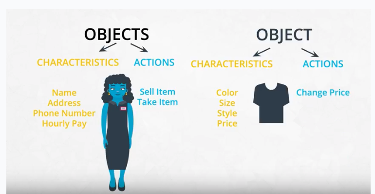
Characteristics and actions in English grammar
You can also think about characteristics and actions is in terms of English grammar. A characteristic corresponds to a noun and an action corresponds to a verb.
Let’s pick something from the real world: a dog. Some characteristics of the dog include the dog’s weight, color, breed, and height. These are all nouns. Some actions a dog can take include to bark, to run, to bite, and to eat. These are all verbs.
Quiz: Characteristics versus actions
Select the characteristics of a tree object. There may be more than one correct answer.
Height
Color
To grow
Width
To fall down
Species
Which of the following would be considered actions for a laptop computer object?
Memory
Width
To turn on
Operating system
To turn off
Thickness
Weight
To erase
Class, object, method, and attribute
Class, object, method, and attribute
Object-oriented programming (OOP) vocabulary
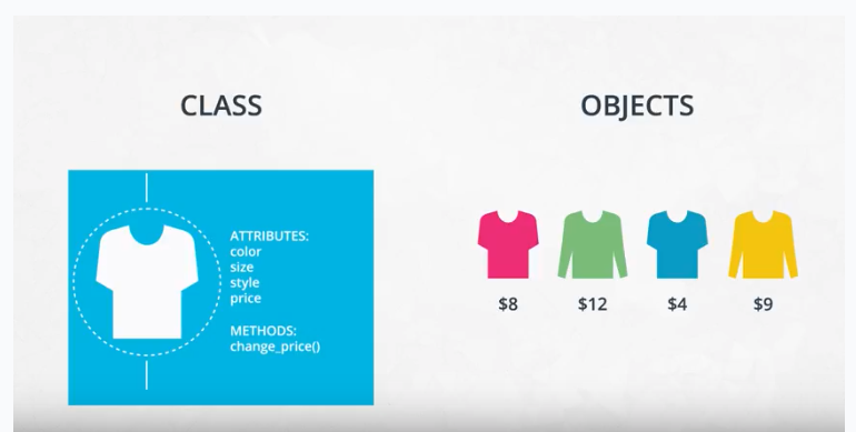
- Class: A blueprint consisting of methods and attributes.
- Object: An instance of a class. It can help to think of objects as something in the real world like a yellow pencil, a small dog, or a blue shirt. However, as you’ll see later in the lesson, objects can be more abstract.
- Attribute: A descriptor or characteristic. Examples would be color, length, size, etc. These attributes can take on specific values like blue, 3 inches, large, etc.
- Method: An action that a class or object could take.
- OOP: A commonly used abbreviation for object-oriented programming.
- Encapsulation: One of the fundamental ideas behind object-oriented programming is called encapsulation: you can combine functions and data all into a single entity. In object-oriented programming, this single entity is called a class.
- Encapsulation allows you to hide implementation details, much like how the
scikit-learnpackage hides the implementation of machine learning algorithms.
In English, you might hear an attribute described as a property, description, feature, quality, trait, or characteristic. All of these are saying the same thing.
Here is a reminder of how a class, an object, attributes, and methods relate to each other.
Match the vocabulary term on the left with the examples on the right.
| TERM | EXAMPLES |
|---|---|
| Object | Stephen Hawking, Angela Merkel, Brad Pitt |
| Class | Scientist, chancellor, actor |
| Attribute | Color, size, shape |
| Method | To rain, to ring, to ripen |
| Value | Gray, large, round |
OOP syntax
Object-oriented programming syntax
In this video, you’ll see what a class and object look like in Python. In the next section, you’ll have the chance to play around with the code. Finally, you’ll write your own class.
Function versus method
In the video above, at 1:44, the dialogue mistakenly calls init a function rather than a method. Why is init not a function?
A function and a method look very similar. They both use the def keyword. They also have inputs and return outputs. The difference is that a method is inside of a class whereas a function is outside of a class.
What is self?
If you instantiate two objects, how does Python differentiate between these two objects?
1 | shirt_one = Shirt('red', 'S', 'short-sleeve', 15) |
That’s where self comes into play. If you call the change_price method on shirt_one, how does Python know to change the price of shirt_one and not of shirt_two?
1 | shirt_one.change_price(12) |
Behind the scenes, Python is calling the change_price method:
1 | def change_price(self, new_price): |
Self tells Python where to look in the computer’s memory for the shirt_one object. Then, Python changes the price of the shirt_one object. When you call the change_price method, shirt_one.change_price(12), self is implicitly passed in.
The word self is just a convention. You could actually use any other name as long as you are consistent, but you should use self to avoid confusing people.
Exercise: OOP syntax practice, part 1
Exercise: Use the Shirt class

You’ve seen what a class looks like and how to instantiate an object. Now it’s your turn to write code that instantiates a shirt object.
You need to download three files for this exercise. These files are located on this page in the Supporting materials section.
Shirt_exercise.ipynbcontains explanations and instructions.Answer.pycontaining solution to the exercise.Tests.pytests for checking your code: You can run these tests using the last code cell at the bottom of the notebook.
Getting started
Open the Shirt Exercise.ipynb notebook file using Jupyter Notebook and follow the instructions in the notebook to complete the exercise.
Supporting Materials
Notes about OOP
Notes about OOP
Set and get methods
The last part of the video mentioned that accessing attributes in Python can be somewhat different than in other programming languages like Java and C++. This section goes into further detail.
The Shirt class has a method to change the price of the shirt: shirt_one.change_price(20). In Python, you can also change the values of an attribute with the following syntax:
1 | shirt_one.price = 10 |
This code accesses and changes the price, color, size, and style attributes directly. Accessing attributes directly would be frowned upon in many other languages, but not in Python. Instead, the general object-oriented programming convention is to use methods to access attributes or change attribute values. These methods are called set and get methods or setter and getter methods.
A get method is for obtaining an attribute value. A set method is for changing an attribute value. If you were writing a Shirt class, you could use the following code:
1 | class Shirt: |
Instantiating and using an object might look like the following code:
1 | shirt_one = Shirt('yellow', 'M', 'long-sleeve', 15) |
In the class definition, the underscore in front of price is a somewhat controversial Python convention. In other languages like C++ or Java, price could be explicitly labeled as a private variable. This would prohibit an object from accessing the price attribute directly like shirt_one._price = 15. Unlike other languages, Python does not distinguish between private and public variables. Therefore, there is some controversy about using the underscore convention as well as get and set methods in Python. Why use get and set methods in Python when Python wasn’t designed to use them?
At the same time, you’ll find that some Python programmers develop object-oriented programs using get and set methods anyway. Following the Python convention, the underscore in front of price is to let a programmer know that price should only be accessed with get and set methods rather than accessing price directly with shirt_one._price. However, a programmer could still access _price directly because there is nothing in the Python language to prevent the direct access.
To reiterate, a programmer could technically still do something like shirt_one._price = 10, and the code would work. But accessing price directly, in this case, would not be following the intent of how the Shirt class was designed.
One of the benefits of set and get methods is that, as previously mentioned in the course, you can hide the implementation from your user. Perhaps, originally, a variable was coded as a list and later became a dictionary. With set and get methods, you could easily change how that variable gets accessed. Without set and get methods, you’d have to go to every place in the code that accessed the variable directly and change the code.
You can read more about get and set methods in Python on this Python Tutorial site.
Attributes
There are some drawbacks to accessing attributes directly versus writing a method for accessing attributes.
In terms of object-oriented programming, the rules in Python are a bit looser than in other programming languages. As previously mentioned, in some languages, like C++, you can explicitly state whether or not an object should be allowed to change or access an attribute’s values directly. Python does not have this option.
Why might it be better to change a value with a method instead of directly? Changing values via a method gives you more flexibility in the long-term. What if the units of measurement change, like if the store was originally meant to work in US dollars and now has to handle Euros? Here’s an example:
Example: Dollars versus Euros
If you’ve changed attribute values directly, you’ll have to go through your code and find all the places where US dollars were used, such as in the following:
1 | shirt_one.price = 10 # US dollars |
Then, you’ll have to manually change them to Euros.
1 | shirt_one.price = 8 # Euros |
If you had used a method, then you would only have to change the method to convert from dollars to Euros.
1 | def change_price(self, new_price): |
For the purposes of this introduction to object-oriented programming, you don’t need to worry about updating attributes directly versus with a method; however, if you decide to further your study of object-oriented programming, especially in another language such as C++ or Java, you’ll have to take this into consideration.
Modularized code
Thus far in the lesson, all of the code has been in Jupyter Notebooks. For example, in the previous exercise, a code cell loaded the Shirt class, which gave you access to the shirt class throughout the rest of the notebook.
If you were developing a software program, you would want to modularize this code. You would put the Shirt class into its own Python script, which you might call shirt.py. In another Python script, you would import the Shirt class with a line like from shirt import Shirt.
For now, as you get used to OOP syntax, you’ll be completing exercises in Jupyter Notebooks. Midway through the lesson, you’ll modularize object-oriented code into separate files.
Exercise: OOP syntax practice, part 2
Exercise: Use the Pants class
Now that you’ve had some practice instantiating objects, it’s time to write your own class from scratch.
This lesson has two parts.
- In the first part, you’ll write a
Pantsclass. This class is similar to theShirtclass with a couple of changes. Then you’ll practice instantiatingPantsobjects. - In the second part, you’ll write another class called
SalesPerson. You’ll also instantiate objects for theSalesPerson.
This exercise requires two files, which are located on this page in the Supporting Materials section.
exercise.ipynbcontainsexplanations and instructions.answer.pycontains solution to the exercise.
Getting started
Open the exercise.ipynb notebook file using Jupyter Notebook and follow the instructions in the notebook to complete the exercise.
Supporting Materials
Commenting object-oriented code
Commenting object-oriented code
Did you notice anything special about the answer key in the previous exercise? The Pants class and the SalesPerson class contained docstrings! A docstring is a type of comment that describes how a Python module, function, class, or method works. Docstrings are not unique to object-oriented programming.
For this section of the course, you just need to remember to use docstrings and to comment your code. It will help you understand and maintain your code and even make you a better job candidate.
From this point on, please always comment your code. Use both inline comments and document-level comments as appropriate.
To learn more about docstrings, see Example Google Style Python Docstrings.
Example Google Style Python Docstrings
Example NumPy Style Python Docstrings
Docstrings and object-oriented code
The following example shows a class with docstrings. Here are a few things to keep in mind:
- Make sure to indent your docstrings correctly or the code will not run. A docstring should be indented one indentation underneath the class or method being described.
- You don’t have to define
selfin your method docstrings. It’s understood that any method will haveselfas the first method input.
1 | class Pants: |
Gaussian class
Gaussian class
Resources for review
The example in the next part of the lesson assumes you are familiar with Gaussian and binomial distributions.
Here are a few formulas that might be helpful:
Gaussian distribution formulas
probability density function:
$$\displaystyle f(x | \mu, \sigma^2) = \frac{1}{\sqrt{2\pi\sigma^2}}e^{-(x - \mu)^2/2\sigma^2}$$
- $\mu$ is the mean
- $\sigma$ is the standard deviation
- $\sigma^2$ is the variance
Binomial distribution formulas
- mean: $\displaystyle \mu = n \times p$
In other words, a fair coin has a probability of a positive outcome (heads) $p = 0.5$. If you flip a coin 20 times, the mean would be $20 * 0.5 = 10$; you’d expect to get 10 heads.
- variance: $\displaystyle \sigma^2 = np(1 - p)$
Continuing with the coin example, $n$ would be the number of coin tosses and $p$ would be the probability of getting heads.
- Standard deviation: $\displaystyle \sigma = \sqrt{np(1-p)}$
In other words, the standard deviation is the square root of the variance.
probability density function
$$\displaystyle f(k, n, p) = \frac{n!}{k!(n-k)!}p^k(1-p)^{(n-k)}$$
Further resources
If you would like to review the Gaussian (normal) distribution and binomial distribution, here are a few resources:
This free Udacity course, Intro to Statistics, has a lesson on Gaussian distributions as well as the binomial distribution.
This free course, Intro to Descriptive Statistics, also has a Gaussian distributions lesson.
There are also relevant Wikipedia articles:
Gaussian Distributions Wikipedia
Binomial Distributions Wikipedia
Quiz
How to Use and Create a Z-Table (Standard Normal Table)
Quiz - Gaussian class
Here are a few quiz questions to help you determine how well you understand the Gaussian and binomial distributions. Even if you can’t remember how to answer these types of questions, feel free to move on to the next part of the lesson; however, the material assumes you know what these distributions are and that you know the basics of how to work with them.
Assume the average weight of an American adult male is 180 pounds, with a standard deviation of 34 pounds. The distribution of weights follows a normal distribution. What is the probability that a man weighs exactly 185 pounds?
0.56
0
0.44
0.059
$\mu = 180, \sigma = 34, \sigma^2 = 34^2 = 1156$
Assume the average weight of an American adult male is 180 pounds, with a standard deviation of 34 pounds. The distribution of weights follows a normal distribution. What is the probability that a man weighs somewhere between 120 and 155 pounds?
0
0.23
0.27
0.19
Now, consider a binomial distribution. Assume that 15% of the population is allergic to cats. If you randomly select 60 people for a medical trial, what is the probability that 7 of those people are allergic to cats?
.01
.14
0
.05
.12
How the Gaussian class works
Exercise: Code the Gaussian class
In this exercise, you will use the Gaussian distribution class for calculating and visualizing a Gaussian distribution.
This exercise requires three files, which are located on this page in the Supporting materials section.
Gaussian_code_exercise.ipynbcontains explanations and instructions.Answer.pycontains the solution to the exercise .Numbers.txtcan be read in by theread_data_file()method.
Getting started
Open the Gaussian_code_exercise.ipynb notebook file using Jupyter Notebook and follow the instructions in the notebook to complete the exercise.
Supporting Materials
Magic methods
Magic methods
Magic methods in code
Exercise: Code magic methods
Exercise: Code magic methods
Extend the code from the previous exercise by using two new methods, add and repr.
This exercise requires three files, which are located on this page in the Supporting materials section.
Magic_methods.ipynbcontains explanations and instructions.Answer.pycontains the solution to the exercise.Numbers.txtcan be read in by the read_data_file() method.
Getting started
Open the Magic_methods.ipynb notebook file using Jupyter Notebook and follow the instructions in the notebook to complete the exercise.
Supporting Materials
Inheritance
Inheritance
Inheritance code
In the following video, you’ll see how to code inheritance using Python.
Check the boxes next to the statements that are true. There may be more than one correct answer.
Inheritance helps organize code with a more general version of a class and then specific children.
Inheritance makes code much more difficult to maintain.
Inheritance can make object-oriented programs more efficient to write.
Updates to a parent class automatically trickle down to its children.
Exercise: Inheritance with clothing
Exercise: Inheritance with clothing
Using the Clothing parent class and two children classes, Shirt and Pants, you will code a new class called Blouse.
This exercise requires two files, which are located on this page in the Supporting materials section.
Inheritance_exercise_clothing.ipynbcontains explanations and instructions.Answer.pycontains the solution to the exercise.
Getting started
Open the Inheritance_exercise_clothing.ipynb notebook file using Jupyter Notebook and follow the instructions in the notebook to complete the exercise.
Supporting Materials
Inheritance Gaussian class
Demo: Inheritance probability distributions
Inheritance with the Gaussian class
This is a code demonstration, so you do not need to write any code.
From the Supporting materials section on this page, download the file calledinheritance_probability_distribution.ipynb
Getting started
Open the file using Jupyter Notebook and follow these instructions:
To give another example of inheritance, read through the code in this Jupyter Notebook to see how the code works.
- You can see the Gaussian distribution code is refactored into a generic distribution class and a Gaussian distribution class.
- The distribution class takes care of the initialization and the
read_data_filemethod. The rest of the Gaussian code is in the Gaussian class. You’ll use this distribution class in an exercise at the end of the lesson.
Run the code in each cell of this Jupyter Notebook.
Supporting Materials
Organizing into modules
Organizing into modules
Windows vs. macOS vs. Linux
Linux, which our Udacity classroom workspaces use, is an operating system like Windows or macOS. One important difference is that Linux is free and open source, while Windows is owned by Microsoft and macOS by Apple.
Throughout the lesson, you can do all of your work in a classroom workspace. These workspaces provide interfaces that connect to virtual machines in the cloud. However, if you want to run this code locally on your computer, the commands you use might be slightly different.
If you are using macOS, you can open an application called Terminal and use the same commands that you use in the workspace. That is because Linux and MacOS are related.
If you are using Windows, the analogous application is called Console. The Console commands can be somewhat different than the Terminal commands. Use a search engine to find the right commands in a Windows environment.
The classroom workspace has one major benefit. You can do whatever you want to the workspace, including installing Python packages. If something goes wrong, you can reset the workspace and start with a clean slate; however, always download your code files or commit your code to GitHub or GitLab before resetting a workspace. Otherwise, you’ll lose your code!
Demo: Modularized code
Demo: Modularized code
This is a code demonstration, so you do not need to write any code.
So far, the coding exercises have been in Jupyter Notebooks. Jupyter Notebooks are especially useful for data science applications because you can wrangle data, analyze data, and share a report all in one document. However, they’re not ideal for writing modular programs, which require separating code into different files.
At the bottom of this page under Supporting materials, download three files.
Gaussiandistribution.pyGeneraldistribution.pyexample_code.py
Look at how the distribution class and Gaussian class are modularized into different files.
The Gaussiandistribution.py imports the Distribution class from the Generaldistribution.py file. Note the following line of code:
1 | from Generaldistribution import Distribution |
This code essentially pastes the distribution code to the top of the Gaussiandistribution file when you run the code. You can see in the example_code.py file an example of how to use the Gaussian class.
The example_code.py file then imports the Gaussian distribution class.
For the rest of the lesson, you’ll work with modularized code rather than a Jupyter Notebook. Go through the code in the modularized_code folder to understand how everything is organized.
Supporting Materials
Advanced OOP topics
Inheritance is the last object-oriented programming topic in the lesson. Thus far you’ve been exposed to:
- Classes and objects
- Attributes and methods
- Magic methods
- Inheritance
Classes, object, attributes, methods, and inheritance are common to all object-oriented programming languages.
Knowing these topics is enough to start writing object-oriented software. What you’ve learned so far is all you need to know to complete this OOP lesson. However, these are only the fundamentals of object-oriented programming.
Use the following list of resources to learn more about advanced Python object-oriented programming topics.
- Python’s Instance, Class, and Static Methods Demystified: This article explains different types of methods that can be accessed at the class or object level.
- Class and Instance Attributes: You can also define attributes at the class level or at the instance level.
- Mixins for Fun and Profit: A class can inherit from multiple parent classes.
- Primer on Python Decorators: Decorators are a short-hand way to use functions inside other functions.
Making a package
Making a package
In the previous section, the distribution and Gaussian code was refactored into individual modules. A Python module is just a Python file containing code.
In this next section, you’ll convert the distribution code into a Python package. A package is a collection of Python modules. Although the previous code might already seem like it was a Python package because it contained multiple files, a Python package also needs an __init__.py file. In this section, you’ll learn how to create this __init__.py file and then pip install the package into your local Python installation.
What is pip?
pip is a Python package manager that helps with installing and uninstalling Python packages. You might have used pip to install packages using the command line: pip install numpy. When you execute a command like pip install numpy, pip downloads the package from a Python package repository called PyPI.
For this next exercise, you’ll use pip to install a Python package from a local folder on your computer. The last part of the lesson will focus on uploading packages to PyPi so that you can share your package with the world.
You can complete this entire lesson within the classroom using the provided workspaces; however, if you want to develop a package locally on your computer, you should consider setting up a virtual environment. That way, if you install your package on your computer, the package won’t install into your main Python installation. Before starting the next exercise, the next part of the lesson will discuss what virtual environments are and how to use them.
Object-oriented programming and Python packages
A Python package does not need to use object-oriented programming. You could simply have a Python module with a set of functions. However, most—if not all—of the popular Python packages take advantage of object-oriented programming for a few reasons:
- Object-oriented programs are relatively easy to expand, especially because of inheritance.
- Object-oriented programs obscure functionality from the user. Consider
scipypackages. You don’t need to know how the actual code works in order to use its classes and methods.
Virtual environments
Python environments
In the next part of the lesson, you’ll be given a workspace where you can upload files into a Python package and pip install the package. If you decide to install your package on your local computer, you’ll want to create a virtual environment. A virtual environment is a silo-ed Python installation apart from your main Python installation. That way you can install packages and delete the virtual environment without affecting your main Python installation.
Let’s talk about two different Python environment managers: conda and venv. You can create virtual environments with either one. The following sections describe each of these environment managers, including some advantages and disadvantages. If you’ve taken other data science, machine learning, or artificial intelligence courses at Udacity, you’re probably already familiar with conda.
Conda
Conda does two things: manages packages and manages environments.
As a package manager, conda makes it easy to install Python packages, especially for data science. For instance, typing conda install numpy installs the numpy package.
As an environment manager, conda allows you to create silo-ed Python installations. With an environment manager, you can install packages on your computer without affecting your main Python installation.
The command line code looks something like the following:
1 | conda create --name [environmentname] |
pip and Venv
There are other environmental managers and package managers besides conda. For example, venv is an environment manager that comes preinstalled with Python 3. pip is a package manager.
pip can only manage Python packages, whereas conda is a language agnostic package manager. In fact, conda was invented because pip could not handle data science packages that depended on libraries outside of Python. If you look at the history of conda, you’ll find that the software engineers behind conda needed a way to manage data science packages (such as NumPy and Matplotlib) that relied on libraries outside of Python.
conda manages environments and packages. pip only manages packages.
To use venv and pip, the commands look something like the following:
1 | python3 -m venv [environmentname] |
Which to choose
Whether you choose to create environments with venv or conda will depend on your use case. conda is very helpful for data science projects, but conda can make generic Python software development a bit more confusing; that’s the case for this project.
If you create a conda environment, activate the environment, and then pip install the distributions package, you’ll find that the system installs your package globally rather than in your local conda environment. However, if you create the conda environment and install pip simultaneously, you’ll find that pip behaves as expected when installing packages into your local environment:
1 | conda create --name [environmentname] pip |
On the other hand, using pip with venv works as expected. pip and venv tend to be used for generic software development projects including web development. For this lesson on creating packages, you can use conda or venv if you want to develop locally on your computer and install your package.
The following video shows how to use venv, which is what we recommend for this project.
Instructions for venv
For instructions about how to set up virtual environments on a macOS, Linux, or Windows machine using the terminal, see Installing packages using pip and virtual environments.
Refer to the following notes for understanding the tutorial:
- If you are using Python 2.7.9 or later (including Python 3), the Python installation should already come with the Python package manager called pip. There is no need to install it.
envis the name of the environment you want to create. You can call env anything you want.- Python 3 comes with a virtual environment package preinstalled. Instead of typing
python3 -m virtualenv env, you can typepython3 -m venv envto create a virtual environment.
Once you’ve activated a virtual environment, you can then use terminal commands to go into the directory where your Python library is stored. Then, you can run pip install.
In the next section, you can practice pip installing and creating virtual environments in the classroom workspace. You’ll see that creating a virtual environment actually creates a new folder containing a Python installation. Deleting this folder removes the virtual environment.
If you install packages on the workspace and run into issues, you can always reset the workspace; however, you will lose all of your work. Be sure to download any files you want to keep before resetting a workspace.
Exercise: Making a package and pip installing
Exercise: Making a package and pip installing
In this exercise, you will convert modularized code into a Python package.
This exercise requires three files, which are located on this page in the Supporting materials section.
Gaussiandistribution.pyGeneraldistribution.py3b_answer_python_package.zipcontains the solution to the exercise.
Instructions
Following the instructions from the previous video, convert the modularized code into a Python package.
On your local computer, you need to create a folder called 3a_python_package. Inside this folder, you need to create a few folders and files:
- A
setup.pyfile, which is required in order to usepip install. - A subfolder called
distributions, which is the name of the Python package. - Inside the
distributionsfolder, you need:- The
Gaussiandistribution.pyfile (provided). - The
Generaldistribution.pyfile (provided). - The
__init__.pyfile (you need to create this file).
- The
Once everything is set up, in order to actually create the package, use your terminal window to navigate into the 3a_python_package folder.
Enter the following:
1 | cd 3a_python_package |
If everything is set up correctly, pip installs the distributions package into the workspace. You can then start the Python interpreter from the terminal by entering:
1 | python |
Then, within the Python interpreter, you can use the distributions package by entering the following:
1 | from distributions import Gaussian |
In other words, you can import and use the Gaussian class because the distributions package is now officially installed as part of your Python installation.
If you get stuck, there’s a solution provided in the Supporting materials section called 3b_answer_python_package .
If you want to install the Python package locally on your computer, you might want to set up a virtual environment first. A virtual environment is a silo-ed Python installation apart from your main Python installation. That way you can easily delete the virtual environment without affecting your Python installation.
If you want to try using virtual environments in this workspace first, follow these instructions:
- There is an issue with the Ubuntu operating system and Python3, in which the
venvpackage isn’t installed correctly. In the workspace, one way to fix this is by running this command in the workspace terminal:conda update python. For more information, see venv doesn’t create activate script python3. Then, enterywhen prompted. It might take a few minutes for the workspace to update. If you are not using Anaconda on your local computer, you can skip this first step. - Enter the following command to create a virtual environment:
python -m venv [venv_name]wherevenv_nameis the name you want to give to your virtual environment. You’ll see a new folder appear with the Python installation namedvenv_name. - In the terminal, enter
source venv_name/bin/activate. You’ll notice that the command line now shows(venv_name)at the beginning of the line to indicate you are using thevenv_namevirtual environment. - Enter pip install
python_package/.That should install your distributions Python package. - Try using the package in a program to see if everything works!
Supporting Materials
- Exercise - Making a package and pip installing
- Generaldistribution
- Gaussiandistribution
- 3b Answer Python Package
Binomial class
Binomial class
Binomial class exercise
In the following video, you’ll get an overview of the binomial class exercise.
Exercise: Binomial class
Exercise: Binomial class
In this exercise, you’ll extend the distributions package with a new class called Binomial.
In the Supporting materials section of this page, there is a .zip file called called 4a_binomial_package.zip. Download and unzip this file.
Inside the folder called 4a_binomial_package, there is another folder and these files:
distributions, which contains the code for the distributions package includingGaussiandistribution.pyandGeneraldistribution.pycode.setup.py, a file needed for building Python packages with pip.test.pyunit tests to help you debug your code.numbers.txtandnumbers_binomial.txt, which are data files used as part of the unit tests.Binomialdistribution.pyandBinomialdistribution_challenge.py. Choose one of these files for completing the exercise.Binomialdistribution.pyincludes more of the code already set up for you. In Binomialdistribution_challenge.py, you’ll have to write all of the code from scratch. Both files contain instructions with TODOS to fill out.
In these files, you only need to change the following:
__init__.py, inside the distributions folder. You need to import the binomial package.- Either
Binomialdistribution.pyorBinomialdistribution_challenge.pyYou also need to put yourBinomialdistribution.pyfile into the distributions folder.
When you’re ready to test out your code, follow these steps:
pip install your distributions package. In the terminal, make sure you are in the4a_binomial_packagedirectory. If not, navigate there by entering the following at the command line:
1 | cd 4a_binomial_package |
- Run the unit tests. Enter the following.
1 | python -m unittest test |
Modify the Binomialdistribution.py code until all the unit tests pass.
If you change the code in the distributions folder after pip installing the package, Python will not know about the changes.
When you make changes to the package files, you’ll need to run the following:
1 | pip install --upgrade |
In the Supporting materials section of this page, there is also a solution in the 4b_answer_binomial_package. Try not to look at the solution until your code passes all of the unit tests.
Supporting Materials
scikit-learn source code
scikit-learn source code
Contributing to a GitHub project
Use the following resources to learn how to contribute to a GitHub project:
Advanced Python OOP topics
Use the following resouces to learn about more advanced OOP topics that appear in the scikit-learn package:
Putting code on PyPi
Putting code on PyPi
PyPi vs. test PyPi
Note that pypi.org and test.pypy.org are two different websites. You’ll need to register separately at each website. If you only register at pypi.org , you will not be able to upload to the test.pypy.org repository.
Remember that your package name must be unique. If you use a package name that is already taken, you will get an error when trying to upload the package.
Summary of the terminal commands used in the video
1 | cd binomial_package_files |
More PyPi resources
This tutorial explains how to distribute Python packages, including more configuration options for your setup.py file. You’ll notice that the Python command to run the setup.py is slightly different, as shown in the following example:
1 | python3 setup.py sdist bdist_wheel |
This command still outputs a folder called dist. The difference is that you will get both a .tar.gz file and a .whl file. The .tar.gz file is called a source archive, whereas the .whl file is a built distribution. The .whl file is a newer type of installation file for Python packages. When you pip install a package, pip firsts look for a .whl file (wheel file); if there isn’t one, it looks for the .tar.gz file.
A .tar.gz file (an sdist) contains the files needed to compile and install a Python package. A .whl file (a built distribution) only needs to be copied to the proper place for installation. Behind the scenes, pip installing a .whl file has fewer steps than installing a .tar.gz file.
Other than this command, the rest of the steps for uploading to PyPi are the same.
Other Links
To learn more about PyPi, see the following resources:
Exercise: Upload to PyPi
Exercise: Upload to PyPi
In this part of the lesson, you’ll practice uploading a package to PyPi.
In the Supporting materials section of this page, there is a zip file called 5_exercise_upload_to_pypi.zip . Download and unzip this file.
The Python package is located in the folder 5_exercise_upload_to_pypi.
You need to create three files:
setup.cfgREADME.mdlicense.txt
You also need to create accounts for the pypi test repository and pypi repository.
Don’t forget to keep your passwords; you’ll need to type them into the command line.
Once you have all the files set up correctly, you can use the following commands on the command line. You need to make the name of the package unique, so change the name of the package from distributions to something else. That means changing the information in setup.py and the folder name.
In the terminal, make sure you are in the 5_exercise_upload_to_pypi directory. If not, navigate there by entering the following at the command line:
1 | cd 5_exercise_upload_to_pypi |
Commands to upload to the PyPi test repository
1 | twine upload --repository-url https://test.pypi.org/legacy/ dist/* |
Command to upload to the PyPi repository
1 | twine upload dist/* |
If you get stuck, rewatch the previous video showing how to upload a package to PyPi.
Supporting Materials
Lesson summary
What we covered in this lesson
- Classes vs. objects
- Methods and attributes
- Magic methods and inheritance
- Python packages
Web Development
Develop a data dashboard using Flask, Boostrap, Plotly and Pandas
Introduction
### Why should a data scientist learn web development?In this course, you are going to use Flask to build a data dashboard. You might be thinking that you already have good tools for visualizing data such as matplotlib, seaborn, or Tableau.
However, the web development skills you’ll learn in this lesson will prepare you for building other types of data science applications. Data scientists are increasingly being asked to deploy their work as an application in the cloud.
For example, consider a project where you build a model that classifies disaster relief messages into categories. With your web development skills, you could turn that model into a web app where you would input a message and display the resulting message category.
As another example, consider a system that recommends movies based on a user’s preferences. Part of the recommendation engine could include a web application that displays recommended products based on a userid. What you learn in this course will set you up for building the web app portion of the recommendation engine.
Lesson Overview
### How to Think about This LessonThe lesson first gives an overview of the three base languages for web development: html, css, and JavaScript. You could take an entire course just on each of these languages. The goal is for you to get comfortable writing at least some code in each language so that you understand the web template files at the end of the lesson. This lesson goes through a lot of information to get you up to speed.
To work with the web template and make a data dashboard, you will only need to write Python code. If you want to customize the dashboard, you can do so with just a few changes to the html code. But the underlying technologies of data dashboard will be css, html, JavaScript, and Python.
Lesson Outline
- Basics of a web app
- html
- css
- javascript
- Front-end libraries
- boostrap
- plotly
- Back-end libraries
- flask
- Deploy a web app to the cloud
Lesson Files
All of the lesson’s exercises are contained in classroom workspaces. You’ll even deploy a web app from the classroom workspace; however, if you prefer to work locally, you can find the lesson files in this data scientist nanodegree GitHub repo.
The Web
Components of a Web App
Front End: - Content: HTML - Design: CSS - Interactions: JavaScript Back End: - Server - DatabaseThe Front End
Front End: HTML
HTML Document Example
Here is an example of HTML code
1 |
|
Explanation of the HTML document
As you progress through the lesson, you’ll find that the <head> tag is mostly for housekeeping like specifying the page title and adding meta tags. Meta tags are in essence information about the page that web crawlers see but users do not. The head tag also contains links to javascript and css files, which you’ll see later in the lesson.
The website content goes in the <body> tag. The body tag can contain headers, paragraphs, images, links, forms, lists, and a handful of other tags. Of particular note in this example are the link tag <a> and the image tag <img>.
Both of these tags link to external information outside of the html doc. In the html code above, the link <a> tag links to an external website called w3schools. The href is called an attribute, and in this case href specifies the link.
The image <img> tag displays an image called “photo.jpg”. In this case, the jpg file and the html document are in the same directory, but the documents do not have to be. The src attribute specifies the path to the image file relative to the html document. The alt tag contains text that gets displaced in case the image cannot be found.
Full List of Tags and How to Use Them
This is a link to one of the best references for html. Use this website to look up html tags and how to use them. W3Schools HTML Tags
In fact, the W3Schools website has a lot of free information about web development syntax.
Checking your HTML
It’s a good idea to check the validity of your HTML. Here is a website that checks your HTML for syntax errors: W3C Validator. Try pasting your HTML code here and running the validator. You can read through the error messages and fix your HTML.
Exercise: HTML
1 |
|
Div and Span
Summary of Div and Span Elements
You can use div elements to split off large chunks of html into sections. Span elements, on the other hand, are for small chunks of html. You generally use span elements in the middle of a piece of text in order to apply a specific style to that text. You’ll see how this works a bit later in the CSS portion of the lesson.
1 | <div> |
IDs and Classes
1 | <div id="top"> |
Exercise: HTML Div, Span, IDs, Classes
1 |
|
Front End: CSS
CSS and this Lesson
To build the data dashboard at the end of this lesson, you won’t need to actually write any CSS. Instead, you’ll use libraries that take care of the CSS for you. In this that, that would be the Bootstrap library.
But if you are interested in understanding what Bootstrap is doing under the hood, then you need to understand how to style a website with CSS. This page has a summary of some important aspects of CSS programming.
What is the Purpose of CSS?
In most professional websites, css is kept in a separate stylesheet. This makes it easier to separate content (html) from style (css). Code becomes easier to read and maintain.
If you’re interested in the history of css and how it came about, here is an interesting link: history of css.
CSS stands for cascading style sheets. The “cascading” refers to how rules trickle down to the various layers of an html tree. For example, you might specify that all paragraphs have the same font type. But then you want to override one of the paragraphs to have a different font type. How does a browser decide which rules apply when there is a conflict? That’s based on the cascade over. You can read more about that here.
Different ways to write CSS
As discussed in the video, there are essentially two ways to write CSS: inline or with a stylesheet.
Inline means that you specify the CSS directly inside of an html tag like so:
1 | <p style="font-size:20px;">This is a paragraph</p> |
Alternatively, you can put the CSS in a stylesheet. The stylesheet can go underneath an html head tag like so:
1 | ... |
Or the css can go into its own separate css file (extension .css). Then you can link to the css file within the html head tag like so:
1 | <head> |
where style.css is the path to the style.css file. Inside the style.css file would be the style rules such as
1 | p { |
CSS Rules and Syntax
CSS is essentially a set of rules that you can use to stylize html. The W3 Schools CSS Website is a good place to find all the different rules you can use. These including styling text, links, margins, padding, image, icons and background colors among other options.
The general syntax is that you:
- select the html element, id, and/or class of interest
- specify what you want to change about the element
- specify a value, followed by a semi-colon
For example
1 | a { |
where a is the element of interest, text-decoration is what you want to change, and none is the value. You can write multiple rules within one set of brackets like:
1 | a { |
You can also select elements by their class or id.
To select by class name, you use a dot like so:
1 | .class_name { |
To select by id name, you use the pound sign:
1 | #id_name { |
You can make more complex selections as well like “select paragraphs inside the div with id “div_top” . If your html looks like this,
1 | <div id="div_top"> |
then the CSS would be like this:
1 | div#div_top p { |
Margins and Padding
The difference between margin and padding is a bit tricky. Margin rules specify a spatial buffer on the outside of an element. Padding specifies an internal spatial buffer.
These examples below show how this works. They use a div element with a border. Here is the div without any margin or padding:
1 | <div style="border:solid red 1px;"> |
Margin
In this case, the div has a margin of 40 pixels. This creates a spatial buffer on the outside of the div element.
1 | <div style="border:solid red 1px;margin:40px;"> |
Padding
This next case has a padding of 40px. In the case of padding, the spatial buffer is internal.
1 | <div style="border:solid red 1px;padding:40px;"> |
Margin and Padding
In this case, the div element has both a margin of 40 pixels and a padding of 40 pixels.
1 | <div style="border:solid red 1px;margin:40px;padding:40px;"> |
Specifying Size: Pixels versus Percent versus EM Units
In CSS there are various ways to define sizes, widths, and heights. The three main ones are pixels, percentages, and em units.
When you use px, you’re defining the exact number of pixels an element should use in terms of size. So
1 | <p style="font-size: 12px;"> |
means the font-size will be exactly 12 pixels.
The percent and em units have a similar function. They dynamically change sizing based on a browser’s default values. For example
1 | <p style="font-size: 100%"> |
means to use the default browser font size. 150% would be 1.5 times the default font size. 50% would be half. Similarly, 1em unit would be 1 x default_font. So 2em would be 2 x default font, etc. The advantage of using percents and em is that your web pages become dynamic. The document adapts to the default settings of whatever device someone is using be that a desktop, laptop or mobile phone.
As an aside, percentages and em units are actually calculating sizes relative to parent elements in the html tree. For example, if you specify a font size in a body tag , then the percentages will be relative to the body element:
1 | <body style="font-size: 20px"> |
This is a paragraph
...Because different browsers might render html and CSS differently, there isn’t necessarily a right or wrong way to specify sizes. This will depend on who will use your website and on what type of devices. You can read more here. You won’t need to worry about all of this because in the web app, you’re going to use a CSS framework that takes care of all of this for you.
Exercise: CSS
1 |
|
1 | /* TODO: |
Front End: Bootstrap Library
Documentation References
Here are some key parts of the Bootstrap documentation for your reference:
- Starter Template
- Column Grid Explanation
- Containers and Responsive Layout
- Images
- Navigation Bars
- Font Colors
Why Bootstrap?
Bootstrap is one of the easier front-end frameworks to work with. Bootstrap eliminates the need to write CSS or JavaScript. Instead, you can style your websites with HTML. You’ll be able to design sleek, modern looking websites more quickly than if you were coding the CSS and JavaScript directly.
Exercise: Bootstrap
1 |
|
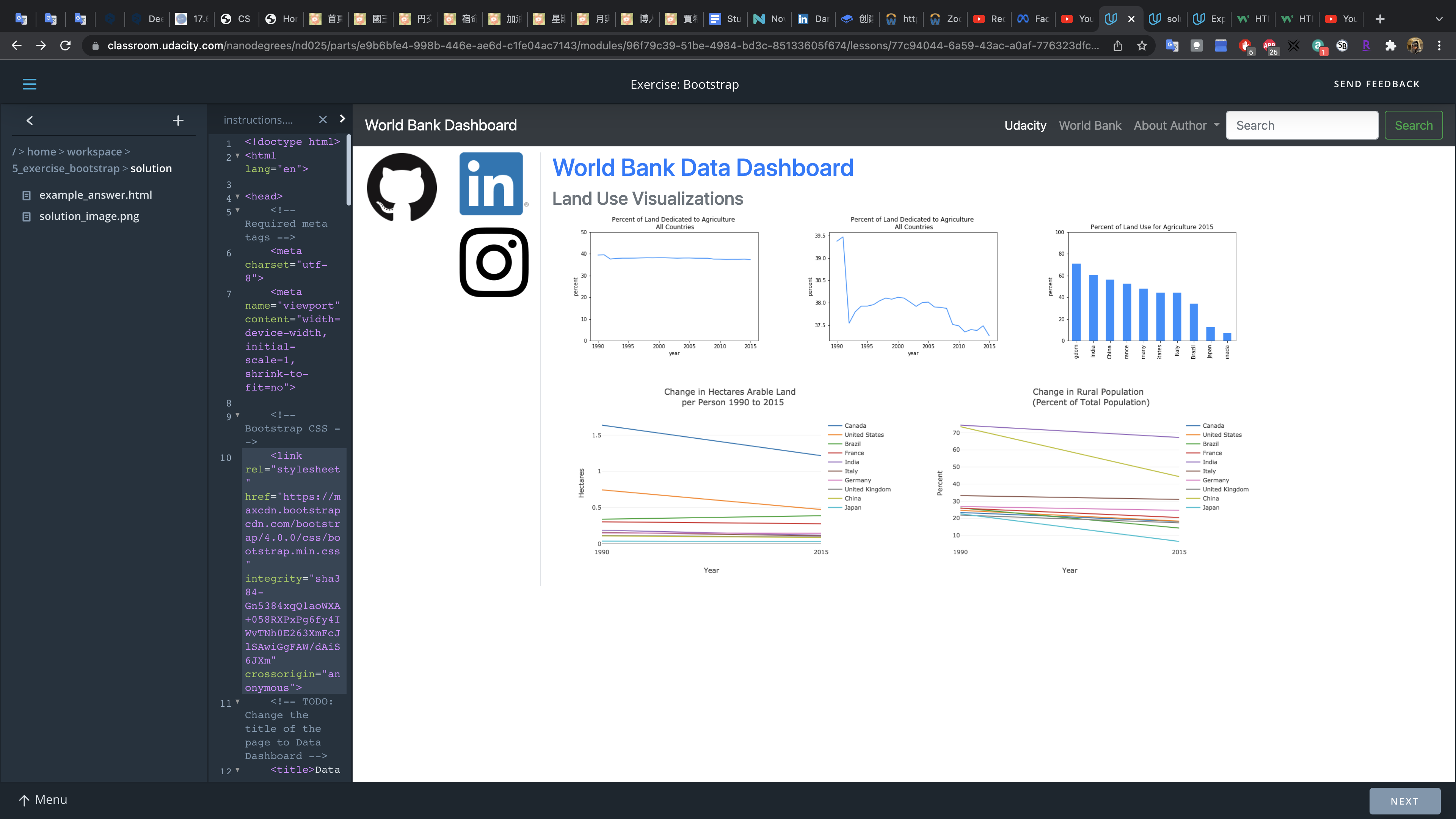
Front End: JavaScript
JavaScript and this Lesson
To build the data dashboard at the end of this lesson, you won’t need to write any JavaScript at all. That’s because you’ll use libraries (Bootstrap and Plotly) that take care of the JavaScript for you.
You won’t need to get into the details of JavaScript syntax, but it’s good to have at least an idea of what is happening under the hood.
What is JavaScript?
- JavaScript is a high level language like Python, PHP, Ruby, and C++. It was specifically developed to make the front-end of a web application more dynamic; however, you can also use javascript to program the back-end of a website with the JavaScript runtime environment node.
- Java and javaScript are two completely different languages that happen to have similar names.
- JavaScript syntax, especially for front-end web development, is a bit tricky. It’s much easier to write front-end JavaScript code using a framework such as jQuery.
Basic JavaScript Syntax
Here are a few rules to keep in mind when writing JavaScript:
- a line of code ends with a semi-colon ;
- () parenthesis are used when calling a function much like in Python
- {} curly braces surround large chunks of code or are used when initializing dictionaries
- [] square brackets are used for accessing values from arrays or dictionaries much like in Python
Here is an example of a JavaScript function that sums the elements of an array.
1 | function addValues(x) { |
What is jQuery?
Jquery is a JavaScript library that makes developing the front-end easier. JavaScript specifically helps with manipulating html elements. The reason we are showing you Jquery is because the Bootstrap library you’ll be using depends on Jquery. But you won’t need to write any Jquery yourself.
Here is a link to the documentation of the core functions in jquery: jQuery API documentation
Jquery came out in 2006. There are newer JavaScript tools out there like React and Angular.
As a data scientist, you probably won’t need to use any of these tools. But if you work in a startup environment, you’ll most likely hear front-end engineers talking about these tools.
jQuery Syntax
The jQuery library simplifies JavaScript quite a bit. Compare the syntax. Compare these two examples from the video for changing the h1 title element when clicking on the image.
This is pure JavaScript code for changing the words in the h1 title element.
1 | function headFunction() { |
This code searches the html document for all h1 tags, grabs the first h1 tag in the array of h1 tags, and then changes the html. Note that the above code is only the function. You’d also have to add an onClick action in the image html tag like so:
1 | <img src="image.jpg" onclick="headFunction()"> |
The jQuery code is more intuitive. Once the document has loaded, the following code adds an onclick event to the image. Once the image is clicked, the h1 tag’s text is changed.
1 | $(document).ready(function(){ |
The dollar sign $ is jQuery syntax that says “grab this element, class or id”. That part of the syntax should remind you somewhat of CSS. For example $(“p#first”) means find the paragraph with id=”first”. Or $(“#first”) would work as well.
Javascript has something called callback function, which can make learning javascript a bit tricky. Callback functions are essentially functions that can be inputs into other functions. In the above code, there is the ready() function that waits for the html document to load. Then there is another function being passed into the ready function. This section function adds an on-click event to an image tag. Then there’s another function passed into the click() function, which changes the h1 text.
Exercise: JavaScript
In the next exercise, you’ll write a bit of jQuery just so that you can see how it works and what it does. This is the only time in the lesson you’ll actually write any JavaScript.
1 | /* |
Front End: Plotly
Chart Libraries
There are many web chart libraries out there for all types of use cases. When choosing a library, you should consider checking whether or not the library is still being actively developed.
d3.js is one of the most popular (and complex!) javascript data visualization libraries. This library is still actively being developed, which you can tell because the latest commit to the d3 GitHub repository is fairly recent.
Other options include chart.js, Google Charts, and nvd3.js, which is built on top of d3.js
Why Plotly
For this lesson, we’ve chosen plotly for a specific reason: Plotly, although a private company, provides open source libraries for both JavaScript and Python.
Because the web app you’re developing will have a Python back-end, you can use the Python library to create your charts. Rather than having you learn more JavaScript syntax, you can use the Python syntax that you already know. However, you haven’t built a back-end yet, so for now, you’ll see the basics of how Plotly works using the JavaScript library. The syntax between the Python and Javascript versions is similar.
Later in the lesson, you’ll switch to the Python version of the Plotly library so that you can prepare visualizations on the back-end of your web app. Yet you could write all the visualization code in JavaScript if you wanted to. Watch the screencast below to learn the basics of how Plotly works, and then continue on to the Plotly exercise.
Here are a few links to some helpful parts of the plotly documentation:
Exercise: Plotly
plot1.js
1 | var year = [1995, 1996, 1997, 1998, 1999, 2000, 2001, 2002, 2003, 2004, 2005, |
plot2.js
1 | var year = [2015]; |
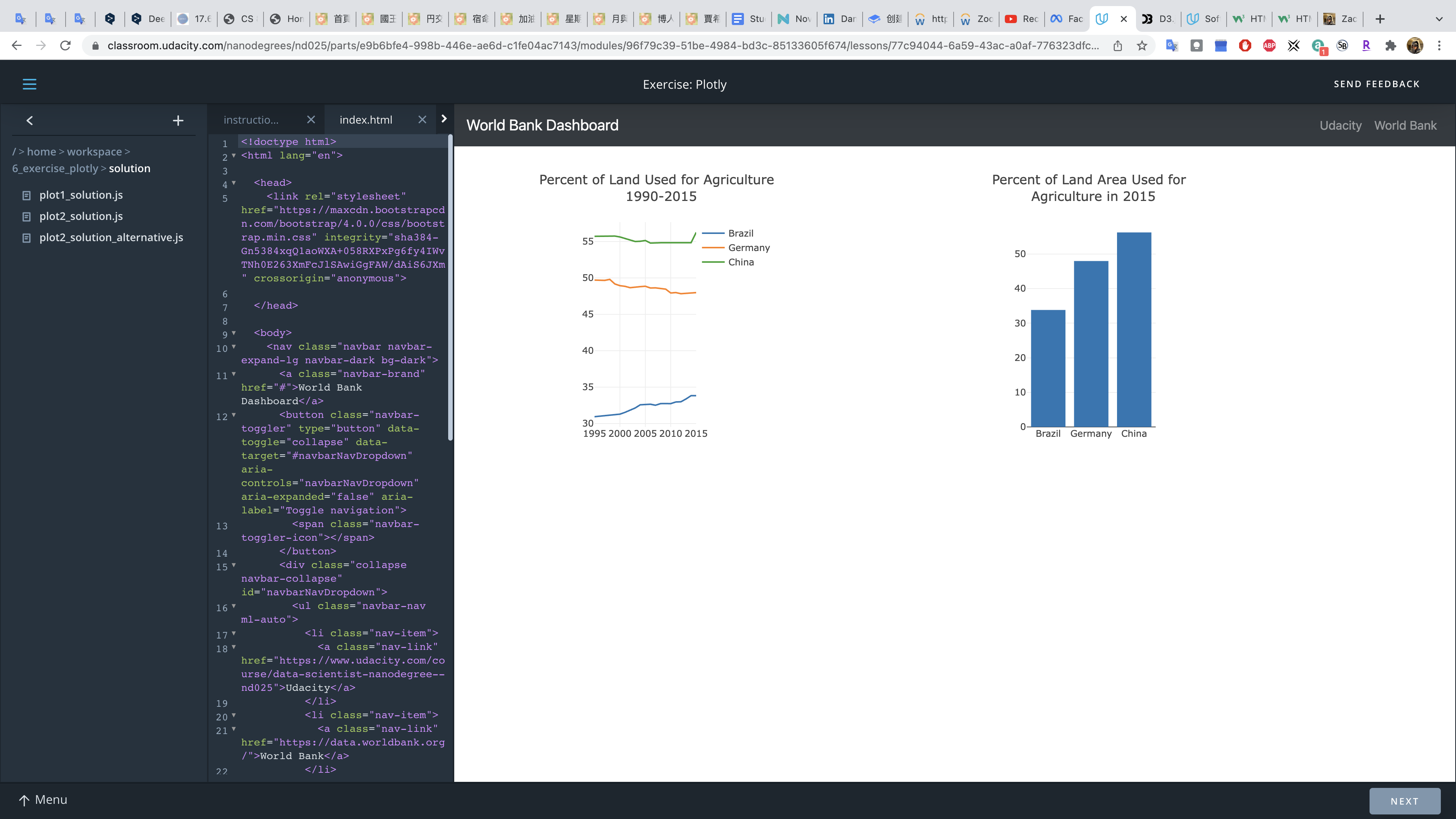
The Backend
In this next part of the lesson, you’ll build a backend using Flask. Because Flask is written in Python, you can use any Python library in your backend including pandas and scikit-learn.
In this part of the lesson, you’ll practice
- setting up the backend
- linking the backend and the frontend together
- deploying the app to a server so that the app is available from a web address
What is Flask?
Flask. A web framework takes care of all the routing needed to organize a web page so that you don’t have to write the code yourself!
When you type “http://www.udacity.com” into a browser, your computer sends out a request to another computer (ie the server) where the Udacity website is stored. Then the Udacity server sends you the files needed to render the website in your browser. The Udacity computer is called a server because it “serves” you the files that you requested.
The HTTP part of the web address stands for Hypter-text Transfer Protocol. HTTP defines a standard way of sending and receiving messages over the internet.
When you hit enter in your browser, your computer says “get me the files for the web page at www.udacity.com”: except that message is sent to the server with the syntax governed by HTTP. Then the server sends out the files via the protocol as well.
There needs to be some software on the server that can interpret these HTTP requests and send out the correct files. That’s where a web framework like Flask comes into play. A framework abstracts the code for receiving requests as well as interpreting the requests and sending out the correct files.
Why Flask?
- First and foremost, you’ll be working with Flask because it is written in Python. You won’t need to learn a new programming language.
- Flask is also a relatively simple framework, so it’s good for making a small web app.
- Because Flask is written in Python, you can use Flask with any other Python library including pandas, numpy and scikit-learn. In this lesson, you’ll be deploying a data dashboard and pandas will help get the data ready.
Continue on to start building the backend.
Backend: Flask
Using Flask in the Classroom Workspace
In the next part of the lesson, you’ll see a classroom workspace. The classroom workspace already has Flask set up for you. So for now, all you need to do to run the Flask app is to open a Terminal and type.
1 | python worldbank.py |
That assumes you are in the default workspace directory within Terminal. That will get the server running.
Seeing your App in the Workspace
Once the server is running, open a new terminal window and type
1 | env | grep WORK |
This command will return the Linux environmental variables that contain information about your classroom workspace. The env command will list all the environmental variables. The | symbol is a pipe for sending output from one command to another. The grep command searches text, so grep WORK will search for any text containing the word WORK.
The command should return two variables:
1 | WORKSPACEDOMAIN=udacity-student-workspaces.com |
Your WORKSPACEID variable will be different but the WORKSPACEDOMAIN should be the same. Now, open a new web browser window, and type the following in the address bar:
1 | http://WORKSPACEID-3001.WORKSPACEDOMAIN |
In this example, that would be: https://viewc7f3319f2-3001.udacity-student-workspaces.com/
DON’T FORGET TO INCLUDE -3001. You should be able to see the web app. The number 3001 represents the port for accessing your web app.
Creating New Pages
To create a new web page, you first need to specify the route in the routes.py as well as the name of the html template.
1 | @app.route('/new-route') |
The route name, function name, and template name do not have to match; however, it’s good practice to make them similar so that the code is easier to follow.
The new_route.html file must go in the templates folder. Flask automatically looks for html files in the templates folder.
What is @app.route?
To use Flask, you don’t necessarily need to know what @app.route is doing. You only have to remember that the path you place inside of @app.route() will be the web address. And then the function you write below @app.route is used to render the correct html template file for the web address.
In Python, the @ symbol is used for decorators. Decorators are a shorthand way to input a function into another function. Take a look at this code. Python allows you to use a function as an input to another function:
1 | def decorator(input_function): |
Running this code will print the string:
I am an input function
Decorators provide a short-hand way of getting the same behavior:
1 | def decorator(input_function): |
This code will print out:
Decorator function
I am an input function
Instead of using a decorator function, you could get the same behavior with the following code:
1 | input_function = decorator(input_function) |
Because @app.route() has the . symbol, there’s an implication that app is a class (or an instance of a class) and route is a method of that class. Hence a function written underneath @app.route() is going to get passed into the route method. The purpose of @app.route() is to make sure the correct web address gets associated with the correct html template. This code
1 | @app.route('/homepage') |
is ensuring that the web address ‘[www.website.com/homepage`](http://www.website.com/homepage%60) is associated with the index.html template.
If you’d like to know more details about decorators and how @app.route() works, check out these tutorials:
Exercise: Flask
File: /home/workspace/1_flask_exercise/worldbankapp/templates/new_route.html
1 |
|
File: /home/workspace/1_flask_exercise/worldbankapp/routes.py
1 | from worldbankapp import app |
Backend: Flask + Pandas
Code from the Screencast
Here is the code from the routes.py file before refactoring.
The data set comes from this link at the World Bank’s data repository: link to dataset
1 | from worldbankapp import app |
Exercise
The next exercise will be after the section on using Plotly, Pandas, and Flask together. For now, the next part of the lesson has the refactored code shown in this screencast so that you can explore it in more detail. You’ll find it in the 2_flask+pandas_example folder.
Backend: Flask + Plotly + Pandas Part 1
In this next video, you’ll see an example of how to pass data from the back end to the front end of the web app. In the next four parts of this lesson, you’ll get a sense for how data and Plotly code can be taken from the back end and, sent to the front end, and then used to render plots on the front end. The goal of these next few videos is to show you how the web template works, which you’ll be using later in the final exercise.
Summary Part 1
The purpose of this section is to give you an idea of how the final web app works in terms of passing information back and forth between the back end and front end. The web template you’ll be using at the end of the lesson will already provide the code for sharing information between the back and front ends. Your task will be to wrangle data and set up the plotly visualizations using Python. But it’s important to get a sense for how the web app works.
In the video above, the data set was sent from the back end to the front end. This was accomplished by including a variable in the render_template() function like so:
1 | data = data_wrangling() |
What this code does is to first load the data using the data_wrangling function from wrangling.py. This data gets stored in a variable called data.
In render_template, that data is sent to the front end via a variable called data_set. Now the data is available to the front_end in the data_set variable.
In the index.html file, you can access the data_set variable using the following syntax:
1 | {{ data_set }} |
You can do this because Flask comes with a template engine called Jinja. Jinja also allows you to put control flow statements in your html using the following syntax:
1 | {% for tuple in data_set %} |
The logic is:
- Wrangle data in a file (aka Python module). In this case, the file is called wrangling.py. The wrangling.py has a function that returns the clean data.
- Execute this function in routes.py to get the data in routes.py
- Pass the data to the front-end (index.html file) using the render_template method.
- Inside of index.html, you can access the data variable with the squiggly bracket syntax
{{ }}
Next
In the next part, you’ll see how to create a Plotly visualization on the back end and then send the visualization code to the front end for rendering.
Backend: Flask + Plotly + Pandas Part 2
In this section, you’ll see how to create a Plotly visualization on the back end and then send the information to the front end for rendering.
Summary Part 2
In the second part, a Plotly visualization was set up on the back-end inside the routes.py file using Plotly’s Python library. The Python plotly code is a dictionary of dictionaries. The Python dictionary is then converted to a JSON format and sent to the front-end via the render_templates method.
Simultaneously a list of ids are created for the plots. This information is also sent to the front-end using the render_template() method.
On the front-end, the ids and visualization code (JSON code) is then used with the Plotly javascript library to render the plots.
In summary:
- Python is used to set up a Plotly visualization
- An id is created associated with each visualization
- The Python Plotly code is converted to JSON
- The ids and JSON are sent to the front end (index.html).
- The front end then uses the ids, JSON, and JavaScript Plotly library to render the plots.
JavaScript or Python
You could actually do all of this with only JavaScript. You would read the data, wrangle the data, and then create the plots all using JavaScript; however, to do all of this in JavaScript, you’d need to learn more about JavaScript programming. Instead, you can use the pandas and Python skills you already have to wrangle data on the back-end.
Backend: Flask + Plotly + Pandas Part 3
Here, the screencast video shows how to make more complex visualizations in Plotly. This example shows a line chart containing a unique line for each country in the data set.
Summary Part 3
In part 3, the code iterated through the data set to create a visualization with multiple lines: one for each country.
The original code for a line chart with a single line was:
1 | graph_one = [go.Scatter( |
To make a visualization with multiple lines, graph_one will be a list of line charts. This was accomplished with the following code:
1 | graph_one = [] |
Next
In the last section of flask, plotly, and pandas, you’ll see how to add more visualizations to the data dashboard. Then, you’ll see some example code and finally you will practice using flask, plotly, and pandas together.
Backend: Flask + Plotly + Pandas Part 4
In this next section, you’ll see how to add more visualizations in the back end code and then render those visualizations on the front end.
Summary Part 4
In the last part, three more visualizations were added to the wrangling Python module. The wrangling included reading in the data, cleaning the data, and preparing the Plotly code. Each visualization’s code was appended to a list called figures. These visualizations were then imported into the routes.py file. This figures list was sent from the back end to the front end via the render_template method. A list of ids were also sent from the back end to the front end.
Then on the front end (index.html), a div was created for each visualization’s id. And with help from the JavaScript Plotly library, each visualization was rendered inside appropriate div.
Beyond a CSV file
Besides storing data in a local csv file (or text, json, etc.), you could also store the data in a database such as a SQL database.
The database could be local to your website meaning that the database file is stored on the same server as your website; alternatively, the database could be stored somewhere else like on a separate database server or with a cloud service like Amazon AWS.
Using a database with your web app goes beyond the scope of this introduction to web development, here are a few resources for using databases with Flask apps:
- Tutorial - Using Databases with Flask
- SQL Alchemy- a Python toolkit for working with SQL
- Flask SQLAlchemy - a Flask library for using SQLAlchemy with Flask
Next Steps
In the next part of the lesson, you can look at the code and try running the web app from the classroom. Then in the next exercise, you’ll practice adding another visualization to the web app.
Exercise: Flask + Plotly + Pandas
Index.html
1 | <head> |
wrangle_data.py
1 | import pandas as pd |
Deployment
Note: In the classroom workspace, do not update the Python, using the
conda update pythoncommand. Consequently, thepip freeze > requirements.txtcommand is also not required in the workspace. We will provide you the requirements.txt file containing the bare minimum package list.
Instructions Deploying from the Classroom
Here is the code used in the screencast to get the web app running:
Create a new folder _web_app_, and move all of the application folders and files to the new folder:
1
2
3cd 5_deployment/
mkdir web_app
mv -t web_app/ data/ worldbankapp/ worldbank.py wrangling_scripts/ requirements.txt runtime.txt[Applicable only for the Local practice. Not for the workspace.] Create a virtual environment and then activate the environment:
1
2
3
4
5
6
7# Update Python
conda update python
# Run the following from the Exercise folder
# Create a virtual environment
python3 -m venv worldbankvenv
# Activate the new environment (Mac/Linux)
source worldbankenv/bin/activateThe new environment will automatically come with Python packages meant for data science. In addition, pip install the specific Python packages needed for the web app
1
pip install flask==0.12.5 pandas==0.23.3 plotly==2.0.15 gunicorn==19.10.0
Install the Heroku command-line tools. The classroom workspace already has Heroku installed.
1
2
3
4# Verify the installation
heroku --version
# Install, if Heroku not present
curl https://cli-assets.heroku.com/install-ubuntu.sh | shFor your local installation, you can refer to the official installation instructions. And then log into heroku with the following command
1
heroku login -i
Heroku asks for your account email address and password, which you type into the terminal and press enter.
The next steps involves some housekeeping:
remove
app.run()from worldbank.pytype
cd web_appinto the Terminal so that you are inside the folder with your web app code.Create a proc file, which tells Heroku what to do when starting your web app:
1
touch Procfile
Then open the Procfile and type:
1
web gunicorn worldbank:app
[Applicable only for the Local practice. Not for the workspace.] Create a requirements.txt file, which lists all of the Python packages that your app depends on:
1
pip freeze > requirements.txt
For workspace users, the requirements.txt is already available in the exercise folder. In addition, we have also provided a runtime.txt file in the exercise folder, that declares the exact Python version number to use. Heroku supports these Python runtimes.
Initialize a git repository and make a commit:
1
2
3
4
5# Run it just once, in the beginning
git init
# For the first time commit, you need to configure the git username and email:
git config --global user.email "you@example.com"
git config --global user.name "Your Name"Whenever you make any changes to your _web_app_ folder contents, you will have to run
git addandgit commitcommands.1
2
3
4
5# Every time you make any edits to any file in the web_app folder
git add .
# Check which files are ready to be committed
git status
git commit -m "your message"Now, create a Heroku app:
1
2
3
4
5heroku create my-app-name --buildpack heroku/python
# For example,
# heroku create sudkul-web-app --buildpack heroku/python
# The output will be like:
# https://sudkul-web-app.herokuapp.com/ | https://git.heroku.com/sudkul-web-app.gitwhere my-app-name is a unique name that nobody else on Heroku has already used. You can optionally define the build environment using the option
--buildpack heroku/pythonTheheroku createcommand should create a git repository on Heroku and a web address for accessing your web app. You can check that a remote repository was added to your git repository with the following terminal command:1
git remote -v
Before you finally push your local git repository to the remote Heroku repository, you will need the following environment variables (kind of secrets) to send along:
1
2
3
4
5# Set any environment variable to pass along with the push
heroku config:set SLUGIFY_USES_TEXT_UNIDECODE=yes
heroku config:set AIRFLOW_GPL_UNIDECODE=yes
# Verify the variables
heroku configIf your code uses any confidential variable value, you can use this approach to send those values secretly. These values will not be visible to the public users. Now, push your local repo to the remote Heroku repo:
1
2
3# Syntax
# git push <remote branch name> <local branch name>
git push heroku mainOther useful commands are:
1
2
3
4
5# Clear the build cache
heroku plugins:install heroku-builds
heroku builds:cache:purge -a <app-name> --confirm <app-name>
# Permanently delete the app
heroku apps:destroy <app-name> --confirm <app-name>
Now, you can type your web app’s address, such as https://sudkul-web-app.herokuapp.com/, in the browser to see the results.
Other Services Besides Heroku
Heroku is just one option of many for deploying a web app, and Heroku is actually owned by Salesforce.com.
The big internet companies offer similar services like Amazon’s Lightsail, Microsoft’s Azure, Google Cloud, and IBM Cloud (formerly IBM Bluemix). However, these services tend to require more configuration. Most of these also come with either a free tier or a limited free tier that expires after a certain amount of time.
Virtual Environments vs. Anaconda
Virtual environments and Anaconda serve a very similar purpose.
Anaconda is a distribution of Python (and the analytics language R) specifically for data science. Anaconda comes installed with a package and environment manager called conda.
To ensure that your app only installs necessary packages, you should create a virtual Python environment. A virtual Python environment is a separate Python installation on your computer that you can easily remove and won’t interfere with your main Python installation. You can create separate environments using conda. These environments automatically come with default Python packages meant for data science. However, there can be additional packages that you’d want to install in the new environment.
When deploying a web app to a server, you should only include the necessary packages for running your web app. Otherwise, you’d be installing Python packages that you don’t need. We have already provided the package list in the requirements.txt in the workspace above. However, you can create one yourself using the pip freeze > requirements.txt command from the new environment.
Creating a Virtual Environment Locally on Your Computer
You can develop your app using the classroom workspace. If you decide to develop your app locally on your computer, you should set up a virtual environment there as well. Different versions of Python have different ways of setting up virtual environments. The env command allows us to create lightweight virtual environments :
1 | # Optional - Update Python installation |
On Windows, the command is;
1 | > py -3 -m venv myvenv |
For more information, read through this link.
Databases for Your App
The web app in this lesson does not need a database. All of the data is stored in CSV files; however, it is possible to include a database as part of a Flask app. One common use case would be to store user login information such as username and password.
Flask is database agnostic meaning Flask can work with a number of different database types. If you are interested in learning about how to include a database as part of a Flask app, here are some resources:
Deployment
In the next part of the lesson, you’ll find a workspace where you can practice deploying the world bank web app. Set up an account on Heroku and then follow the instructions shown in this part of the lesson.
You’ll need to use a different name for the web app since the one used in this lesson is already taken.
Supporting Materials
Lesson Summary
Portfolio Exercise: Deploy a Data Dashboard
Introduction
Portfolio Exercise: Deploy a Data Dashboard
Personal portfolios are an excellent way to demonstrate your knowledge and creativity. In fact, they are little by little becoming a must-have for people working in the tech industry. In this portfolio building exercise, you will create a data dashboard using Bootstrap, Plotly, Flask and Heroku.
Note that a portfolio exercise like this is not reviewed. So you will not submit your work on this, and you do not need to complete this assignment in order to graduate.
Your main job will be to write Python code that reads in data, cleans the data, and then uses the data to make Plotly visualizations. This is your opportunity to show off your Python coding ability and visualization encoding skills.
In the next part of the lesson, you’ll find a workspace where you can develop the web app. Note that there is also an optional advanced version of the project where you’re encouraged to pull data from an API. You’ll see in this lesson that there are a few sections with “[advanced version]” in the title. If you’d like to do the advanced version, then you’ll want to go through this entire lesson before starting to develop your app.
General Instructions
Develop and deploy a data dashboard. The Web Development lesson has all of the information you need. If you are new to web development, you might have to go back to the concepts and rewatch some of the videos. The “deployment” parts of the lesson should be especially helpful. The video in that part of the lesson shows how to deploy a web app to Heroku. And the associated exercise has a complete, functioning web app with visualizations.
Most of the work will involve:
- Wrangling your chosen data set to get the data in the format you want
- Writing Python code to read in the data set and set up Plotly plots
- Tweaking HTML so that the website has the design and information that you want.
We are providing a template that uses the Bootstrap library and Flask framework. The template is the same one used to build the app in the course except the name of the app has been changed. In the template, everything has the generic name “myapp” instead of “worldbankapp”. The template is set up so that you can use pandas for loading the data and Python to create the dictionaries needed for plotly.
You’ll only need to modify the following files:
- wrangle_data.py
- index.html
Although the front-end is already set up for you, you should change the links and titles in index.html. If you want to add more visualizations or remove visualizations, you’ll need to adjust the front-end code in index.html accordingly. That will involve adding or removing rows and columns in the HTML file.
For deployment, you can use a back-end service like Heroku.
How to Build the App
You’ll find a workspace in the next part of the lesson. The workspace already contains the template code with a working web app. The web app has a back-end and front-end. Recall that you can run the web app from the workspace:
To run the app from the workspace, open a terminal and type env | grep WORK. Note the WORKSPACEDOMAIN and WORKSPACEID. To start the web app, type python myapp.py.
You can open a new browser window and go to the address: http://WORKSPACESPACEID-3001.WORKSPACEDOMAIN replacing WORKSPACEID and WORKSPACEDOMAIN with your values.
However, there is no data for the visualizations. You’ll need to write a Python script that reads in the data files of your choosing and sets up the plots for Plotly. The process will be exactly the same as the one presented in the web development course.
If you need to upload any files to the workspace, you can do so by clicking on the plus (+) sign and choosing “add file” or “add folder”.
The template code is also available on GitHub as part of the data scientist nanodegree term 2 repo.
Test your app in the workspace to make sure that everything is working. You’ll see that if you start the app without modifying any of the code, the app currently works.
You should also save your work to a GitHub or GitLab repository so that you can use your code as part of your professional portfolio.
Once you’re ready to deploy the app, don’t forget to remove the app.run() line of code in the myapp.py file (In the web development lesson, myapp.py was called worldbank.py). You’ll need to add a Procfile and requirements.txt file as well. Follow the instructions in the web development lesson to learn how to deploy the app from the classroom. And always comment your code :-)!
Also, at the end of this page you’re reading, you’ll find information about a more advanced version of the data dashboard that you can build.
Steps
Here is a reminder of the steps you’ll need to do:
- find a data set or a few data sets that you’re interested in
- explore and clean the data set
- put the data into a csv file or files - you can use pandas or spreadsheet software to do this
- upload your data sets to the correct folder
- write a Python script to read in the data set and set up the Plotly visualizations
- set up a virtual environment and install the necessary libraries to run your app
- run your web app locally to make sure that everything works
- deploy the app to Heroku or some other back-end service
Where to Build the Web App
We are providing a workspace containing a web app template. You can use this template to build and deploy your web app within the classroom.
The classroom has an Ubuntu Linux environment. Developing the app locally on macOS should be very similar. On a Windows machine, the commands are slightly different and you’ll need to use the command prompt. This link contains a comparison of MS-DOS vs Linux commands.
To install the Heroku command line interface on a Windows machine, follow the instructions here on the Heroku website.
Advanced Version of the Exercise
If you’d like an extra challenge, consider using an API to obtain your data. API stands for Application Programming Interface. An API provides a convenient way for two applications to communicate with each other. To be more concrete you can pull data directly from the World Bank API, clean the data in the back-end using pandas, and then display the results on your front-end. This would be instead of using a csv file for your data.
The benefit is that if the data ever changes, your web app will automatically have the correct data. Many companies provide APIs for accessing their data including Facebook, Twitter, Google among others. As an example, here is an API for pulling data about DVDs, movies, books, and games.
After the workspace, you’ll find a set of concepts that explain how to use the World Bank API. Go through that material if you’d like an extra challenge for building your web app.
APIs [advanced version]
What is an API?
Instead of downloading World Bank data via a csv file, you’re going to download the data using the World Bank API.
API is an acronym that stands for application programming interface. API’s provide a standardized way for two applications to talk to each other. For this project, the applications communicating with each other are the server application where World Bank stores data and your web application.
If you wanted to pull data directly from the World Bank’s server, you’d have to know what database system the World Bank was using. You’d also need permission to log in directly to the server, which would be a security risk for the World Bank. And if the World Bank ever migrated its data to a new system, you would have to rewrite all of your code again.
The API sits between your web app and the World Bank server. And the API allows you to execute code on the World Bank server without getting direct access.
All sorts of companies have public facing APIs including Facebook, Twitter, Google and Pinterest. You can pull data from these companies to create your own applications.
In the next section, you’ll get practice using Python to pull data from the World Bank API. This will set you up for creating the web app with data from the API instead of using data from a csv file.
APIs Besides the World Bank
All types of companies have APIs. Some of these APIs are only for internal company use while other APIs help the public consume data. A few examples of public APIs include the Twitter API, the Google Maps API, the Facebook Graph API, and the US Government Data APIs.
In addition, oftentimes you can find open source libraries or development kits for connecting to an API. For example, here is an open source Python development kit for the Facebook Graph API.
Some APIs might be used for pulling data from a database. But other APIs are for adding data to a database. For example, you might make an application that automatically tweets the current weather. In that case, you would use the Twitter API to post a tweet, which in reality inserts a tweet into Twitter’s database.
Using an API
In the next few parts of the lesson, you’ll see how to use the World Bank API. This API is relatively straightforward to use. Each API, however, will have a different set up and only allow you to take certain actions. In general, you send a request via a web url that specifies the information you want. You receive data back typically in XML or JSON.
The XML standard was developed in the 1970s and 1980s and soon became a common way to transfer data over the web. JSON was developed in the mid 1990s. Over time, JSON has increased in popularity relative to XML perhaps because JSON is easier to parse.
Some APIs require authentication; essentially the company with the API gives you ‘credentials’ so that they can track how you are using the API and ensure you have the proper permissions.
Some APIs might let you extract data from a database. Other APIs might even let you insert data into a database depending on the use case. Most APIs include extensive documentation so that you can figure out how to use APIs.
If you ever can’t figure out how to use an API, search online for examples. You can search for something like, “Examples for using the World Bank API” or “Examples for using the Facebook API”.
Move on to the next section to see how to use the World Bank API and incorporate it into a web app.
World Bank API [advanced version]
The World Bank API
REST Architecture
REST is a software architecture for the web. You don’t need to understand how REST works in order to use an API. but you will see the term used quite frequently when working with APIs. Modern web APIs are often called RESTFul to indicate that they conform to a REST Architecture.
World Bank API
Here is the website where the csv files were downloaded for the World Bank web app: World Bank Indicator Data
And here is the link to the World Bank API documenation: World Bank API Documentation
One tricky aspect of working with the World Bank API is that it only gives back 50 results at a time. There is an option called per_page that allows you to return up to 1000 results. However, some queries might have more than 1000 results. That’s where the page option comes into play. You’ll notice that at the very beginning of the data, there is a variable called page and another one called pages. If page=1 and pages=4, then you’d need to write 4 queries with the option page=1, page=2, page=3 and page=4.
Next, you’ll practice pulling data from the API using Python code.
Python and APIs [advanced version]
World Bank Data Dashboard [advanced version]
Link to the Code
You can find code for this data dashboard here on GitHub.
How the Filter Works
This version of the web app has a filter made with a form. When you check the boxes on the form and click submit, the form gets submitted to the index.html page. It’s essentially a circle where the index.html loads, the form gets submitted to index.html itself, and then index.html loads again. With a web form, you could also submit the form to a different web page.
On the back-end, routes.py can access the information that was submitted with the web form; the front-end receives information about which boxes were checked.
Code your Project
Start working on your project! Go back to the “Workspace Portfolio Exercise” with the template code. You’ll find it earlier in this Portfolio Exercise lesson. Here are a few APIs that you might find interesting to work with:
Many government and city agencies have APIs where you can access city data.