Udacity Data Engineering
Home Page
References
Introduction
Roles of Data Engineer
Course Roadmap
- Data Engineering
- Data Pipelines
- ETL (Extract Transform Load) Pipelines
- NLP Pipelines
- Text Processing
- Modeling
- Machine Learning Pipelines
- Scikit-learn pipelines
- Feature Union
- Grid Search
- Data Engineering Project
- Classify disaster response messages
- Skills: data pipelines, NLP pipelines, machine learning pipelines, supervised learning
Project Review
Project Preview
In this project you’re going to be analyzing thousands of real messages provided by Figure 8, sent during natural disasters either via social media or directly to disaster response organizations.
- You’ll build an ETL pipeline that processes message and category data from csv files and load them into a SQLite database, which your machine learning pipeline will then read from to create and save a multi-output supervised learning model.
- Then, your web app will extract data from this database to provide data visualizations and use your model to classify new messages for 36 categories.
Machine learning is critical to helping different organizations understand which messages are relevant to them and which messages to prioritize. During these disasters is when they have the least capacity to filter out messages that matter, and find basic methods such as using key word searches to provide trivial results. In this course, you’ll learn the skills you need in ETL pipelines, natural language processing, and machine learning pipelines to create an amazing project with real world significance.
ETL Pipelines
Introduction
Data Pipelines: ETL vs ELT
Data pipeline is a generic term for moving data from one place to another. For example, it could be moving data from one server to another server.
ETL
An ETL pipeline is a specific kind of data pipeline and very common. ETL stands for Extract, Transform, Load. Imagine that you have a database containing web log data. Each entry contains the IP address of a user, a timestamp, and the link that the user clicked.
What if your company wanted to run an analysis of links clicked by city and by day? You would need another data set that maps IP address to a city, and you would also need to extract the day from the timestamp. With an ETL pipeline, you could run code once per day that would extract the previous day’s log data, map IP address to city, aggregate link clicks by city, and then load these results into a new database. That way, a data analyst or scientist would have access to a table of log data by city and day. That is more convenient than always having to run the same complex data transformations on the raw web log data.
Before cloud computing, businesses stored their data on large, expensive, private servers. Running queries on large data sets, like raw web log data, could be expensive both economically and in terms of time. But data analysts might need to query a database multiple times even in the same day; hence, pre-aggregating the data with an ETL pipeline makes sense.
ELT
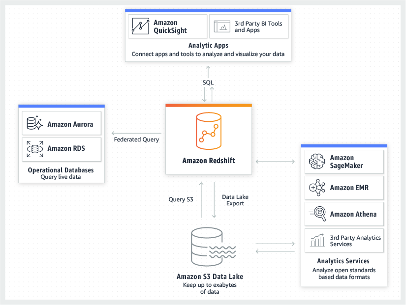
ELT (Extract, Load, Transform) pipelines have gained traction since the advent of cloud computing. Cloud computing has lowered the cost of storing data and running queries on large, raw data sets. Many of these cloud services, like Amazon Redshift, Google BigQuery, or IBM Db2 can be queried using SQL or a SQL-like language. With these tools, the data gets extracted, then loaded directly, and finally transformed at the end of the pipeline.
However, ETL pipelines are still used even with these cloud tools. Oftentimes, it still makes sense to run ETL pipelines and store data in a more readable or intuitive format. This can help data analysts and scientists work more efficiently as well as help an organization become more data driven.
Lesson Overview
Outline of the Lesson
- Extract data from different sources such as:
- csv files
- json files
- APIs
- Transform data
- combining data from different sources
- data cleaning
- data types
- parsing dates
- file encodings
- missing data
- duplicate data
- dummy variables
- remove outliers
- scaling features
- engineering features
- Load
- send the transformed data to a database
- ETL Pipeline
- code an ETL pipeline
This lesson contains many Jupyter notebook exercises where you can practice the different parts of an ETL pipeline. Some of the exercises are challenging, but they also contain hints to help you get through them. You’ll notice that the “transformation” section is relatively long. You’ll oftentimes hear data scientists say that cleaning and transforming data is how they spend a majority of their time. This lesson reflects that reality.
Big Data Courses at Udacity
“Big Data” gets a lot of buzz these days, and it is definitely an important part of a data engineer’s and, sometimes, a data scientists’s work. With “Big Data”, you need special tools that can work on distributed computer systems.
This ETL course focuses on the practical fundamentals of ETL. Hence, you’ll be working with a local data set so that you do not need to worry about learning a new tool. Udacity has other courses where the primary focus is on tools used for distributed data sets.
Here are links to other big data courses at Udacity:
- Intro to Hadoop and MapReduce
- Deploying a Hadoop Cluster
- Real-time Analytics with Apache Storm
- Big Data Analytics in Health Care
How to Tackle the Exercises
s
This course assumes you have experience manipulating data with the Pandas library, which is covered in the data analyst nanodegree. Some of these transformation exercises are challenging. The most challenging exercises are marked (challenging). If an exercise is marked as a challenge, it means you’ll get something out of solving it, but it’s not essential for understanding the lesson material or for getting through the final project at the end of this data engineering course.
Throughout the exercises, you might have to read the pandas documentation or search outside the classroom for how to do a certain processing technique. That is not just expected but also encouraged. As a data scientist professional, you will oftentimes have to research how to do something on your own much like what software engineers do. See this answer on Quora about how often do people use stackoverflow when working on data science projects?.
Use Google and other search engines when you’re not sure how to do something!
What You Will do in the Next Section
In the next section of the lesson, you’ll learn about the extract portion of an ETL pipeline. You’ll get practice with a series of exercises. These exercises are relatively brief and focus on extracting, or in other words, reading in data from different sources. The goal is to familiarize yourself with different types of files and see how the same data can be formatted in different ways.
For a review of pandas, click on the “Extracurricular” section of the classroom. Open the Prerequisite: Python for Data Analysis course, and go to Lesson 7: Pandas.
World Bank Datasets
In the next section, you’ll find a series of exercises. These are relatively brief and focus on extracting, or in other words, reading in data from different sources. The goal is to familiarize yourself with different types of files and see how the same data can be formatted in different ways. This lesson assumes you have experience with pandas and basic programming skills.
This lesson uses data from the World Bank. The data comes from two sources:
- World Bank Indicator Data - This data contains socio-economic indicators for countries around the world. A few example indicators include population, arable land, and central government debt.
- World Bank Project Data - This data set contains information about World Bank project lending since 1947.
Both of these data sets are available in different formats including as a csv file, json, or xml. You can download the csv directly or you can use the World Bank APIs to extract data from the World Bank’s servers. You’ll be doing both in this lesson.
The end goal is to clean these data sets and bring them together into one table. As you’ll see, it’s not as easy as one might hope. By the end of the lesson, you’ll have written an ETL pipeline to extract, transform, and load this data into a new database.
The goal of the lesson is to combine these data sets together so that you can run a linear regression model predicting World Bank Project total costs. You will not actually build the model; instead, you will get the data ready so that a data analyst or data scientist could more easily build the model.
Match the World Bank data set with the type of information it contains
| INFORMATION | DATASET |
|---|---|
| gross domestic product | indicator dataset |
| money spent to build a bridge in Nepal | project dataset |
| World population | indictor dataset |
| a project to help African farmers save water | project dataset |
Summary
Nice work! The indicator data set has statistics about countries all over the world. The projects data set has information about World Bank projects.Extract
Overview of the Extract Part of the Lesson
Summary of the data file types you’ll work with
CSV files
CSV stands for comma-separated values. These types of files separate values with a comma, and each entry is on a separate line. Oftentimes, the first entry will contain variable names. Here is an example of what CSV data looks like. This is an abbreviated version of the first three lines in the World Bank projects data csv file.
1 | id,regionname,countryname,prodline,lendinginstr |
JSON
JSON is a file format with key/value pairs. It looks like a Python dictionary. The exact same CSV file represented in JSON could look like this:
1 | [{"id":"P162228","regionname":"Other","countryname":"World;World","prodline":"RE","lendinginstr":"Investment Project Financing"},{"id":"P163962","regionname":"Africa","countryname":"Democratic Republic of the Congo;Democratic Republic of the Congo","prodline":"PE","lendinginstr":"Investment Project Financing"},{"id":"P167672","regionname":"South Asia","countryname":"People\'s Republic of Bangladesh;People\'s Republic of Bangladesh","prodline":"PE","lendinginstr":"Investment Project Financing"}] |
Each line in the data is inside of a squiggly bracket {}. The variable names are the keys, and the variable values are the values.
There are other ways to organize JSON data, but the general rule is that JSON is organized into key/value pairs. For example, here is a different way to represent the same data using JSON:
XML
Another data format is called XML (Extensible Markup Language). XML is very similar to HTML at least in terms of formatting. The main difference between the two is that HTML has pre-defined tags that are standardized. In XML, tags can be tailored to the data set. Here is what this same data would look like as XML.
1 | <ENTRY> |
XML is falling out of favor especially because JSON tends to be easier to navigate; however, you still might come across XML data. The World Bank API, for example, can return either XML data or JSON data. From a data perspective, the process for handling HTML and XML data is essentially the same.
SQL databases
SQL databases store data in tables using primary and foreign keys. In a SQL database, the same data would look like this:
| id | regionname | countryname | prodline | lendinginstr |
|---|---|---|---|---|
| P162228 | Other | World;World | RE | Investment Project Financing |
| P163962 | Africa | Democratic Republic of the Congo;Democratic Republic of the Congo | PE | Investment Project Financing |
| P167672 | South Asia | People's Republic of Bangladesh;People's Republic of Bangladesh | PE | Investment Project Financing |
Text Files
This course won’t go into much detail about text data. There are other Udacity courses, namely on natural language processing, that go into the details of processing text for machine learning.
Text data present their own issues. Whereas CSV, JSON, XML, and SQL data are organized with a clear structure, text is more ambiguous. For example, the World Bank project data country names are written like this
1 | Democratic Republic of the Congo;Democratic Republic of the Congo |
In the World Bank Indicator data sets, the Democratic Republic of the Congo is represented by the abbreviation “Congo, Dem. Rep.” You’ll have to clean these country names to join the data sets together.
Extracting Data from the Web
In this lesson, you’ll see how to extract data from the web using an APIs (Application Programming Interface). APIs generally provide data in either JSON or XML format.
Companies and organizations provide APIs so that programmers can access data in an official, safe way. APIs allow you to download, and sometimes even upload or modify, data from a web server without giving you direct access.
Match the data with its format
| DATA | FORMAT |
|---|---|
| {‘players’ :5, ‘date’:’Jul 5 1999’} | json |
| players, date 5, Jul 5 1999 | csv |
<entry><players>5</players><date>July 5 1999</date></entry> |
xml |
Exercise: CSV
Exercise: JSON and XML
Exercise: SQL Database
Data Management With Python, SQLite, and SQLAlchemy
Exercise: SQL Database
Text Data
Text data can come in different forms. A text file (.txt), for example, will contain only text. As another example, a data set might contain text for one or more variables. In the world bank projects data set, the regionname, countryname, theme and sector variables contain text.
Analyzing text is a big topic that is covered in other Udacity courses on Natural Language Processing. For the purposes of this lesson on ETL pipelines, pandas is automatically “extracting” text data when reading in a csv, xml or json file.
Text data will be more important in the Transform stage of an ETL pipeline, which comes later in the lesson.
Exercise: APIs
Transform
Transforming Data:
- Combining data & Cleaning data
- Working with encodings
- Removing duplicate rows
- Dummy variables
- Remove outliers
- Normalize Data
- Engineer new features
Overview of the Transform Part of the Lesson
True or False? Data scientists never transform data; transforming data is the job of a data engineer.
True
False
Combining Data
Pandas Resources for Quick Review
Exercise: Combining Data
Cleaning Data
Look Out For
- Missing Values
- Inconsistencies
- Duplicate Data
- Incorrect encodings
Exercise: Cleaning Data
Exercise: Data Types
Exercise: Parsing Dates
Matching Encodings
1 | from encodings.aliases import aliases |
1 | # import the chardet library |
Exercise: Matching Encodings
Missing Data
In the video, I say that a machine learning algorithm won’t work with missing values. This is essentially correct; however, there are a couple of situations where this isn’t quite true. For example, if you had a categorical variable, you could keep the NULL value as one of the options.
Like if theme_2 could have a value of agriculture, banking, or NULL, you might encode this variable as 0, 1, 2 where the value 2 stands in for the NULL value. You could do something similar for one-hot encoding where the theme_2 variable becomes 3 true/false features: theme_2_agriculture, theme_2_banking, theme_2_NULL. You could have to make sure that this improves your model performance.
There are also implementations of some machine learning algorithms, such as gradient boosting decision trees that can handle missing values.
Missing Data - Delete
Missing Data - Impute
Imputation
- Mean Substitution
- Forward Fill, Backward Fill
Exercise: Imputation
SQL, optimization, and ETL - Robert Chang Airbnb
Take a break from all that coding and watch an interview excerpt with Robert Chang, a data scientist at AirBnB. Robert is a data scientist with a deep interest in data engineering. He starts talking about the importance of SQL and discusses optimizing ETL pipelines.
- Understanding data modeling:
- Data warehouse design
- Data tales using star schema
- the notion of a fact table or dimension table
- Data backfilling
- ETL pipelines
- Airflow
Duplicate Data
Exercise: Duplicate Data
Dummy Variables
When to Remove a Feature
As mentioned in the video, if you have five categories, you only really need four features. For example, if the categories are “agriculture”, “banking”, “retail”, “roads”, and “government”, then you only need four of those five categories for dummy variables. This topic is somewhat outside the scope of a data engineer.
In some cases, you don’t necessarily need to remove one of the features. It will depend on your application. In regression models, which use linear combinations of features, removing a dummy variable is important. For a decision tree, removing one of the variables is not needed.
Exercise: Dummy Variables
Outliers - How to Find Them
Outlier Detection Resources [Optional]
Here are a couple of links to outlier detection processes and algorithms. Since this is an ETL course rather than a statistics course, you don’t need to read these in order to complete the lesson.
statistical and machine learning methods for outlier detection
One or two dimensions
- Using visualization to detect outliers
Statistical Methods for Outliers Detection
- Z-Scores
- Tukey Method
- Using ML techniques like PCA to reduce the data to one or two dimensions
- Clustering methods
Tukey Rule
- Q1 = 0.25 quantile
- Q3 = 75% quantile
- IQR = Q3 - Q1
- Max Value = Q3 + IQR * 1.5
- Min Value = Q1 - IQR * 1.5
Exercise: Outliers Part 1
Outliers - What to do
- Consider does the outliers influence the model performance before removing them.
Exercise: Outliers Part 2
AI and Data Engineering - Robert Chang Airbnb
In this interview expert, Robert Chang discusses the AI Hierarchy of Needs and where data engineering comes into play.
Scaling Data
- Normalization / Feature Scaling: Changing the numerical range of data
- Normalization: scaling a set of values so that the range if between zero and one.
- Standardization: scaling a set of values so that they have a mean of zero and a standard deviation of one. The general shape of the distribution remains the same, which means the information contained in the data hasn’t changed. However, the mean and standard deviation has been standardized.
Normalization
To normalize data, you take a feature, like gdp, and use the following formula
$\displaystyle x_{normalized} = \frac{x - x_{min}}{x_{max} - x_{min}}$
where
- x is a value of gdp
- x_max is the maximum gdp in the data
- x_min is the minimum gdp in the data
Assume you have a set of data from 0 to 100.
Normalized:
- 100: (100 - 0) / 100 = 1
- 75: (75 - 0) / 100 = 0.75
- 50: (50 - 0) / 100 = 0.5
- 25: (25 - 0) / 100 = 0.25
- 0: (0 - 0) / 100 = 0
As we can see, every number from the dataset remains the same location as the original dataset. But the scale switched from [0, 100] to [0, 1].
Standardization
$\displaystyle x_{standardized} = \frac{x - \overline{x}}{S}$
Exercise: Scaling Data
Feature Engineering
Making New Features:
- Creating categorical variables from numerical variables
- Multiplying features together
- Gathering more data
Exercise: Feature Engineering
Load
Links to Other Data Storage Systems
Overview of the Load Part of the Lesson
Exercise: Load
Putting it All Together
Overview of the Final Exercise
Exercise: Putting it All Together
Lesson Summary
Lesson Recap
- Prepare data pipelines
- ETL pipelines
- Pulling data from a source
- Transforming data
- Loading data
NLP Pipelines
NLP and Pipelines
- Text Processing
- Cleaning
- Normalization
- Tokenization
- Stop Word Removal
- Part of Speech Tagging
- Named Entity Recognition
- Stemming and Lemmatization
- Feature Extraction
- Bag of Words
- TF-IDF
- Word Embeddings
- Modeling
How How NLP Pipelines Works
Text Processing -> Features Extraction -> Modeling
- Text Processing: Take raw input text, clean it, normalize it, and convert it into a form that is suitable for feature extraction.
- Feature Extraction: Extract and produce feature representations that are appropriate for the type of NLP task you are trying to accomplish and the type of model you are planning to use.
- Modeling: Design a statistical or machine learning model, fit its parameters to training data, use an optimization procedure, and then use it to make predictions about unseen data.
Text Processing Overview
The first chunk of this lesson will explore the steps involved in text processing, the first stage of the NLP pipeline.
Why Do We Need to Process Text?
Source: https://en.wikipedia.org/wiki/Kingfisher
- Extracting plain text: Textual data can come from a wide variety of sources: the web, PDFs, word documents, speech recognition systems, book scans, etc. Your goal is to extract plain text that is free of any source specific markup or constructs that are not relevant to your task.
- Reducing complexity: Some features of our language like capitalization, punctuation, and common words such as a, of, and the, often help provide structure, but don’t add much meaning. Sometimes it’s best to remove them if that helps reduce the complexity of the procedures you want to apply later.
What Text Processing Will You Do in This Lesson?
You’ll prepare text data from different sources with the following text processing steps:
- Cleaning: to remove irrelevant items, such as HTML tags
- Normalizing: by converting to all lowercase and removing punctuation
- Tokenization: Splitting text into words or tokens
- Stop Word Removal: Removing words that are too common, also known as stop words
- Part of Speech Tagging / Named Entity Recognition: Identifying different parts of speech and named entities
- Stemming and Lemmatization: Converting words into their dictionary forms, using stemming and lemmatization
After performing these steps, your text will capture the essence of what was being conveyed in a form that is easier to work with.
Stage 1: Text Processing
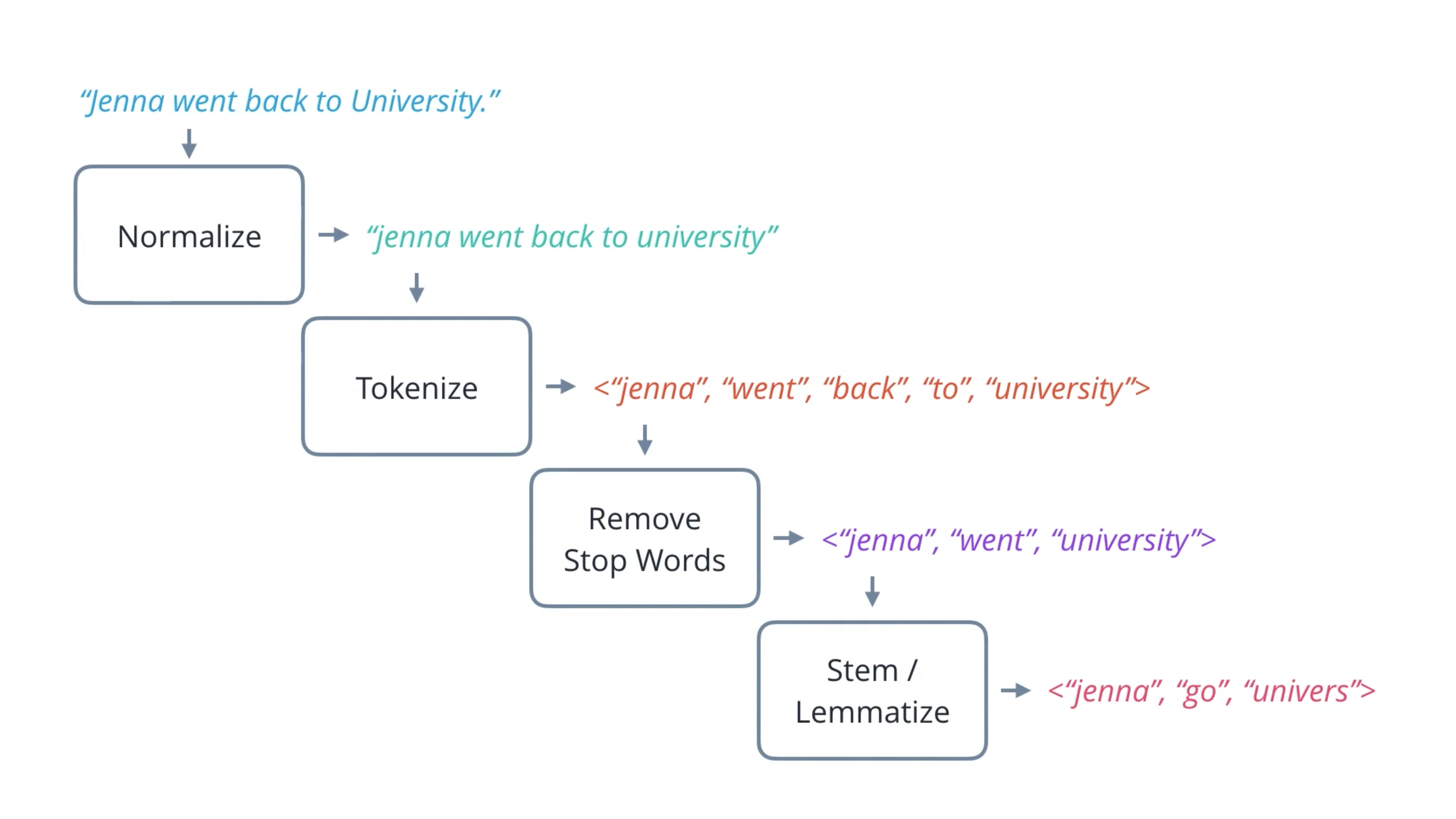
- Normalization: Replace punctuation with a space. Lower all words.
- Tokenization: Split sentence into a sequence of words.
- Stop Word Removal: Remove stop words (the uninformative words).
- Stemming and Lemmatization
Cleaning
Let’s walk through an example of cleaning text data from a popular source - the web. You’ll be introduced to helpful tools in working with this data, including the requests library, regular expressions, and Beautiful Soup.
Note: The website used in this example has since been updated with a new layout. In the next page, you’ll work through the steps shown here for the new web page.
Documentation for Python Libraries:
Notebook: Cleaning
Normalization
Is it better to just remove punctuation characters, or replace each with a space?
Remove
Replace with a space
- Lower the text
- Punctuation Removal
Notebook: Normalization
Tokenization
Reference:
-
nltk.tokenizepackage: http://www.nltk.org/api/nltk.tokenize.html
NLTK is better for NLP rather then using re for normalization. For example, . in Dr. Shen will not be removed by NLTK.
Additionally, NLTK supports splitting text into sentences as well as words.
NLTK has some modules for special text such as # in tweets are tags.
Notebook: Tokenization
Stop Word Removal
Notebook: Stop Word Removal
Part-of-Speech Tagging
Note: Part-of-speech tagging using a predefined grammar like this is a simple, but limited, solution. It can be very tedious and error-prone for a large corpus of text, since you have to account for all possible sentence structures and tags!
There are other more advanced forms of POS tagging that can learn sentence structures and tags from given data, including Hidden Markov Models (HMMs) and Recurrent Neural Networks (RNNs).
Named Entity Recognition
1 | brew install python-tk |
This one doesn’t work.
1 | pip install tk |
Notebook: POS and NER
Stemming and Lemmatization
Notebook: Stemming and Lemmatization
Text Processing Summary
Stage 2: Feature Extraction
Feature Extraction depends on ML models and tasks:
- WordNet: transform text into symbolic nodes with relationships between them for graph based model
- Statistical Model: for statistical model
- Bag of Words
| Feature Extraction Methods | Scale | Part Tasks | Model |
|---|---|---|---|
| WordNet | Word | Word-sense disambiguation, Text classification, Machine translation | Graph Based Model |
| Bag-of-words, Doc2vec, TF-IDF | Document | Spam detection, Sentiment analysis | Statistical Model |
| Word2Vec, GloVe | Word | Text generation, Machine translation | Statistical Model |
Bag of Words
A set of documents is known as a corpus, and this gives the context for the vectors to be calculated.
Collect words from every document then save them (like lists) are in low efficiency.
The better way is to collect all of the unique words (like a set), then count the number of word occurrence for every document, which called term frequency. Then make a table for them, which called Document-Term Matrix.
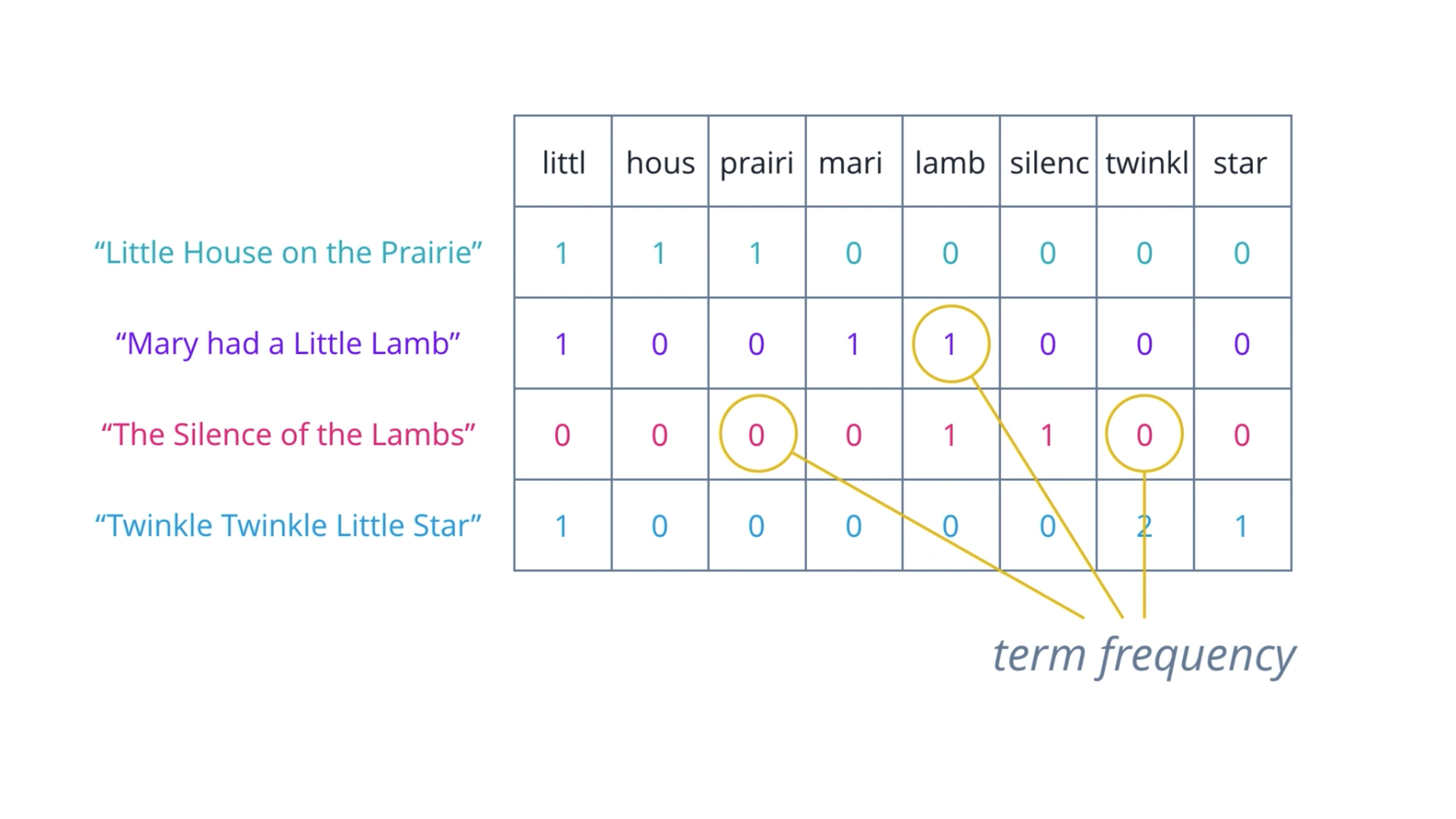
Document-Term Matrix
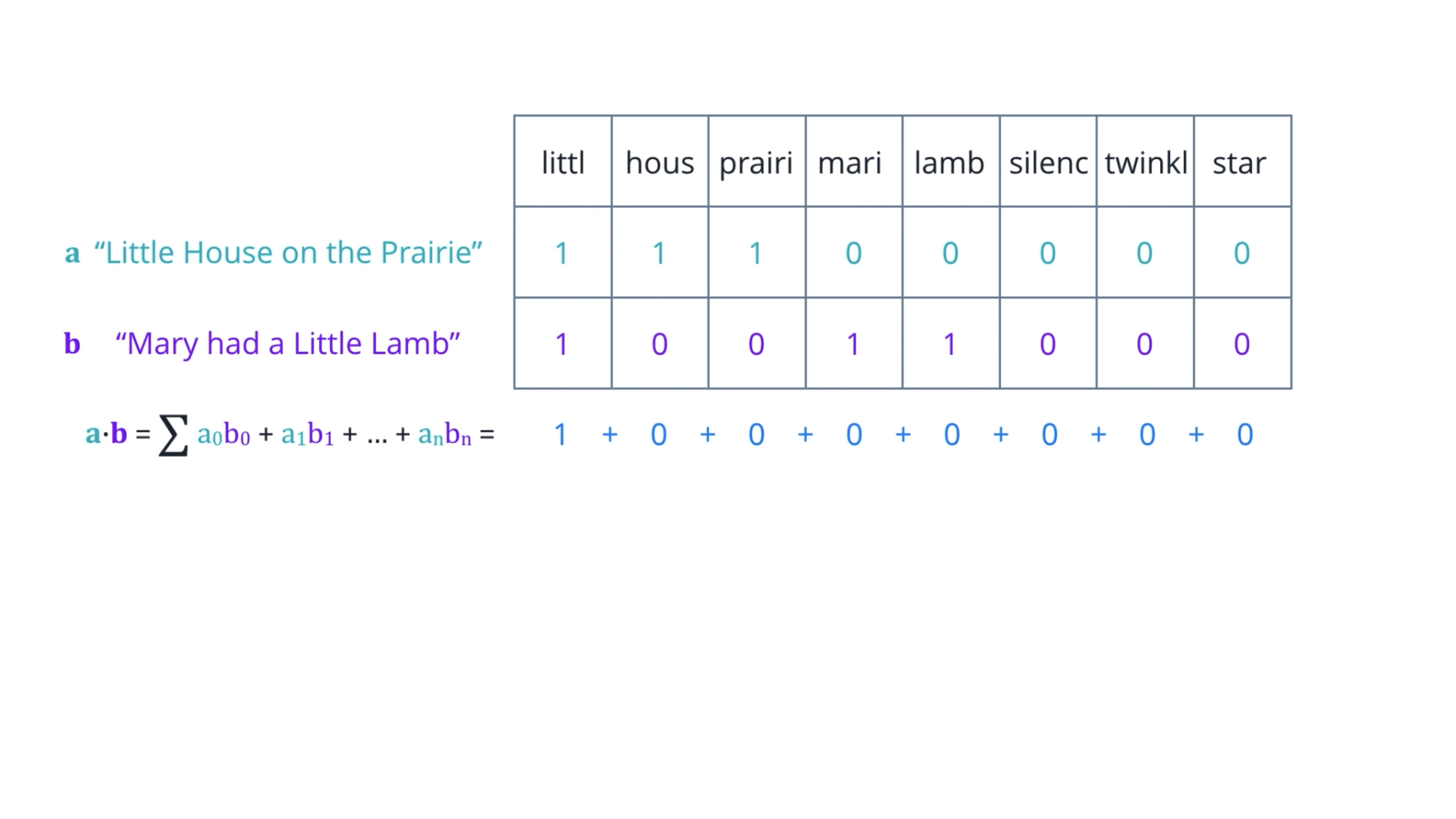
Dot product: compute two row vectors, which is the sum of the products of corresponding elements.
However, dot product only captures the portions of overlap. It is not affected by other values that are not common.
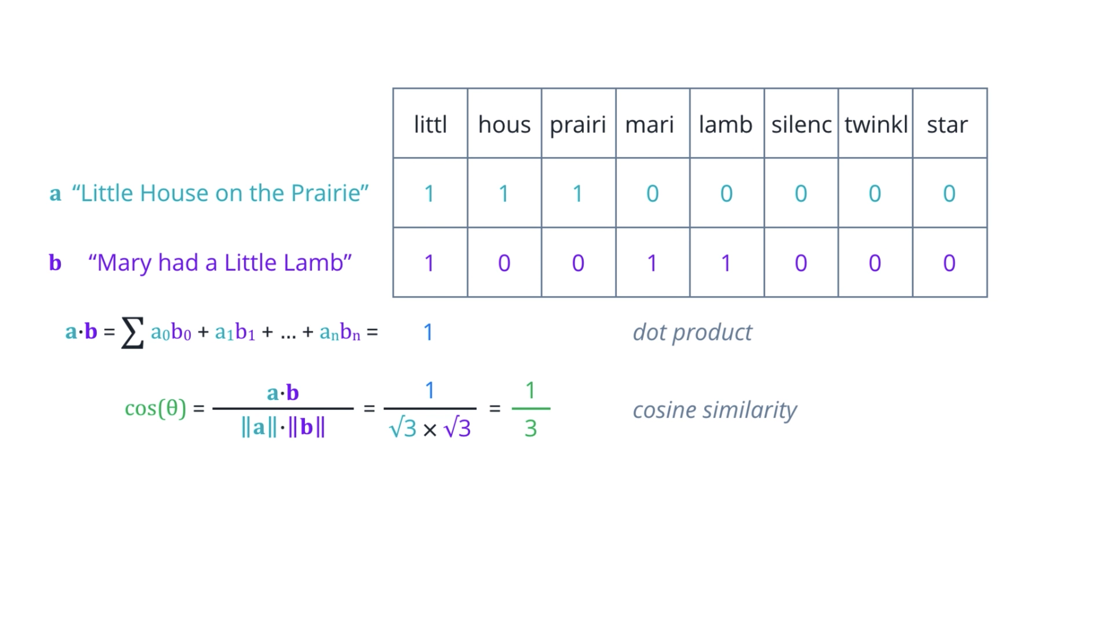
Cosine similarity:
Divide the dot product of two vectors by the product of their magnitudes or Euclidean norms.
If you think of these vectors as arrows in some n-dimensional space, then this is equal to the cosine of the angle theta between them.
Identical vectors have cosine equals one.
Orthogonal vectors have cosine equals zero.
And for vectors that are exactly opposite, it is minus one.
So, the value always range nicely between one for most similar, to minus one, most dissimilar.
TF-IDF
One limitation of the bag of words approach is that it treats every word as being equally important.
Whereas intuitively, we know that some words occur frequently within a corpus.
Therefore, we can compensate for this by counting the number of documents in which each word occurs which called document frequency.
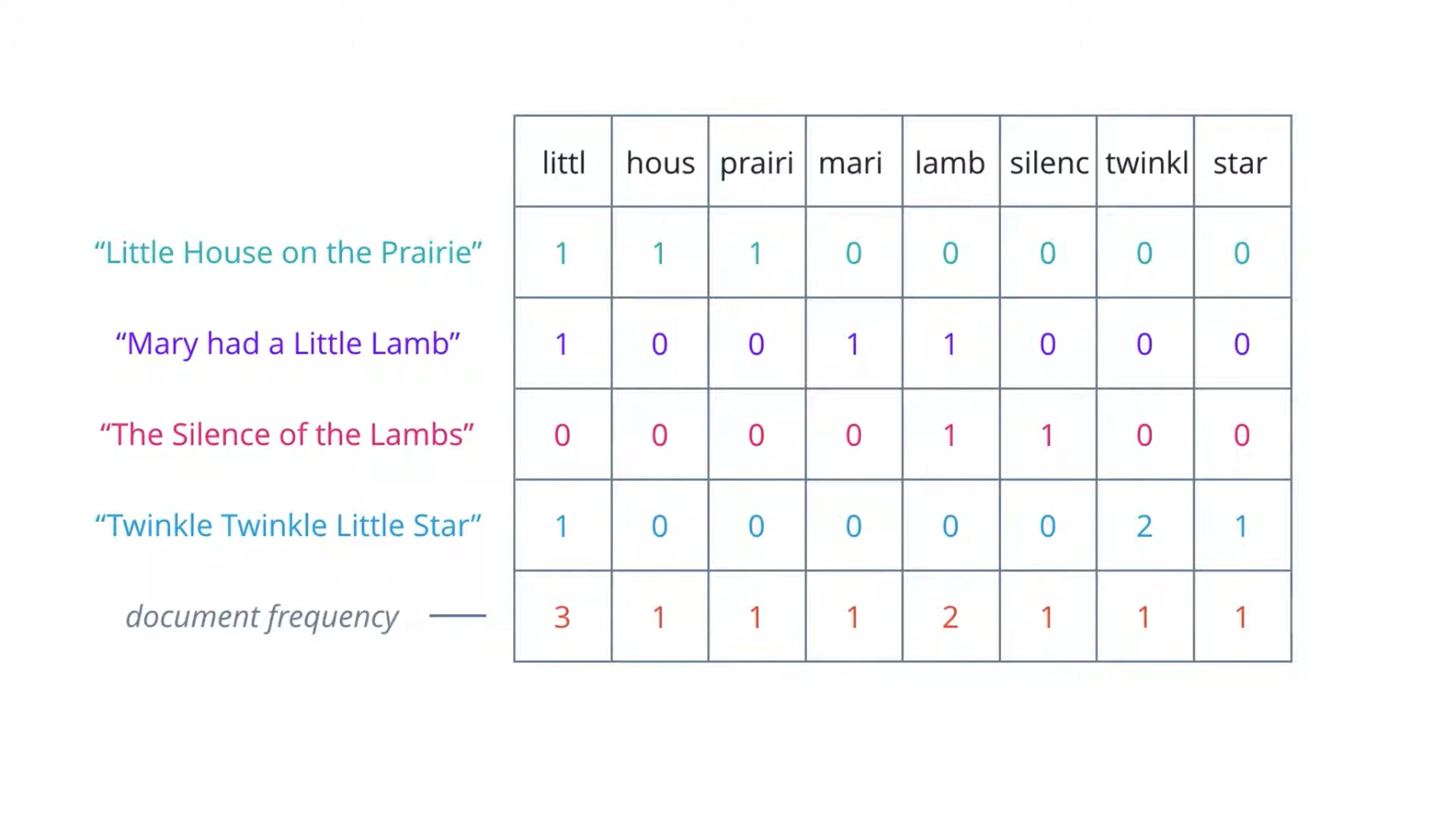
Then dividing the term frequencies by the document frequency of that term.
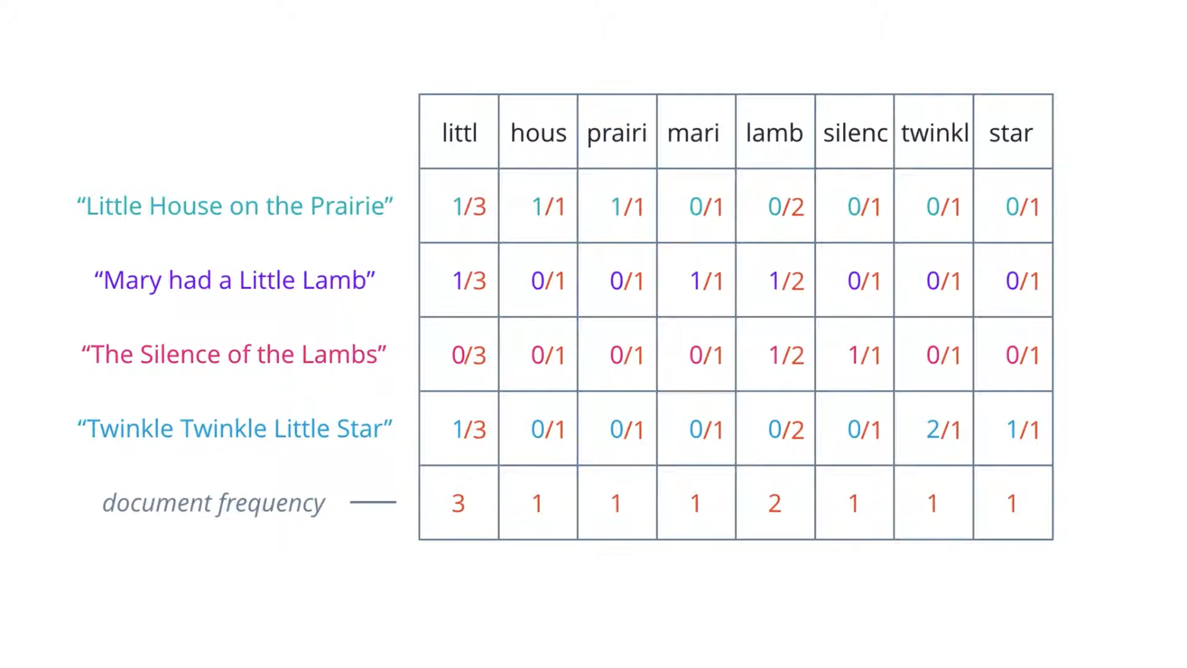
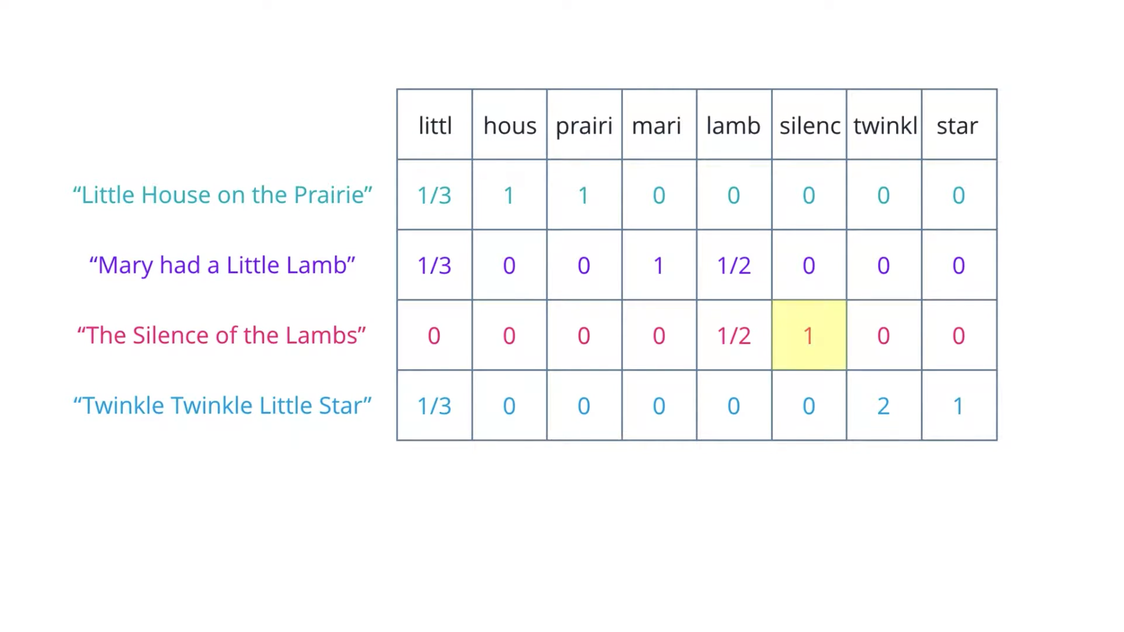
This gives us a metric that is proportional to the frequency of occurrence of a term in a document, but inversely proportional to the number of documents it appears in.
It highlights the words that are more unique to a document and thus better for characterizing it. For example, the highlighted 1 here represents silenc is unique among the four documents – it only appear in the third document for once.
TF-IDF: Term Frequency - Inverse Document Frequency
It’s simply the product of two weights.
The most commonly used form of TF-IDF defines term frequency as the raw count of a term T in a document D, divided by the total number of terms in D. Inverse document frequency as the logarithm of the total number of documents in the collection D, divided by the number of documents where T is present.
Several variations exist, that try to normalize or smooth the resulting values or prevent edge cases such as divide by zero errors.
Overall TF-IDF is an innovative approach to assigning weights to words, that signify their relevance in documents.
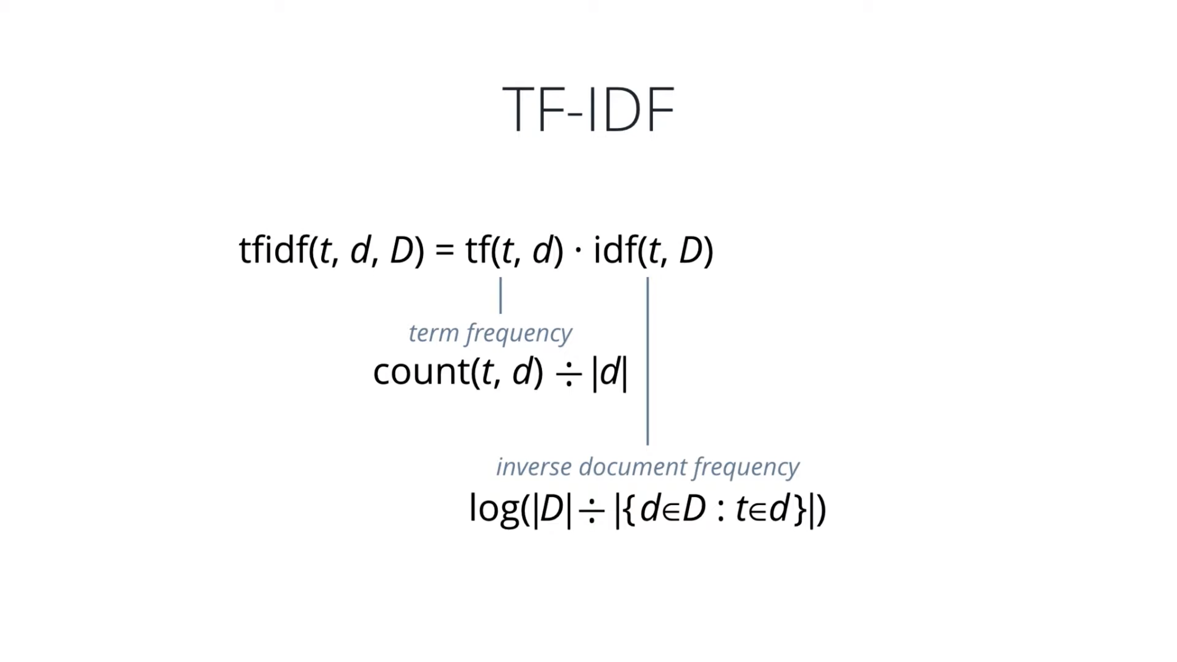
Term Frequency, $tf(t, d)$, is the frequency of term $t$,
$$\displaystyle tf(t, d) = \frac{f_{t, d}}{\sum_{t’ \in d}f_{t’, d}}$$
where $f_{t, d}$ is the raw count of a term in a document, i.e., the number of times that term $t$ occurs in document $d$. There are various other ways to define term frequency:
- the raw count itself: $\displaystyle tf(t, d) = f_{t, d}$
- Boolean frequencies: $\displaystyle tf(t, d) = 1$
- term frequency adjusted for document length: $\displaystyle tf(t, d) = f_{t, d} \div \textnormal{(number of words in d)}$
- logarithmmically scaled frequency: $\displaystyle tf(t, d) = log(1 + f_{t, d})$
- augmented frequency, to prevent a bias towards longer documents, e.g. raw frequency divided by the raw frequency of the most occurring term in the document: $\displaystyle tf(t, d) = 0.5 + 0.5 \cdot \frac{f_{t, d}}{max{f_{t’, d}:t’ \in d}}$
The inverse document frequency is a measure of how much information the word provides, i.e., if it’s common or rare across all documents. It is the logarithmically scaled inverse fraction of the documents that contain the word (obtained by dividing the total number of documents by the number of documents containing the term, and then taking the logarithm of that quotient):
$$idf(t, D) = log \frac{N}{|d \in D:t \in d|}$$
with
- $N$: total number of documents in the corpus $N = |D|$
- $|{d \in D:t \in d}|$: number of documents where the term $t$ appears (i.e., $tf(t, d) \neq 0$. If the term is not in the corpus, this will lead to a division-by-zero. It is therefore common to adjust the denominator to $1 + |{d \in D:t \in d}|$.
Term frequency–Inverse document frequency
Then tf–idf is calculated as
$$tfidf(t, d, D) = td(t, d) \cdot idf(t, D)$$
A high weight in tf–idf is reached by a high term frequency (in the given document) and a low document frequency of the term in the whole collection of documents; the weights hence tend to filter out common terms. Since the ratio inside the idf’s log function is always greater than or equal to 1, the value of idf (and tf–idf) is greater than or equal to 0. As a term appears in more documents, the ratio inside the logarithm approaches 1, bringing the idf and tf–idf closer to 0.
| weighting scheme | document term weight | query term weight |
|---|---|---|
| 1 | ||
| 2 | ||
| 3 |


Notebook: Bag of Words and TF-IDF
One-Hot Encoding
Word Embeddings
Stage 3: Modeling
Modeling
The final stage of the NLP pipeline is modeling, which includes designing a statistical or machine learning model, fitting its parameters to training data, using an optimization procedure, and then using it to make predictions about unseen data.
The nice thing about working with numerical features is that it allows you to choose from all machine learning models or even a combination of them.
Once you have a working model, you can deploy it as a web app, mobile app, or integrate it with other products and services. The possibilities are endless!
Model: Word2Vec
Word2Vec is the most popular examples of word embeddings used in practice.
The model predicts the given word, given neighboring words, or vice versa.
- Continuous Bag of Words(CBoW): given neighboring words.
- Continuous Skip-gram: given the middle word.
Word2Vec: Properties
- Robust, distributed representation.
- Vector size independent of vocabulary.
- Train once, store in lookup table.
- Deep learning ready.
Model: GloVe
GloVe tries to directly optimize the vector representation of each word just using co-occurrence statistics, unlike Word2Vec which sets up an ancillary prediction task.
Embeddings for Deep Learning
Transfer Learning:
It’s common to use some pre-trained layers from an existing network, like Alex or BTG 16 and only learn the later layers for time saving.
t-SNE
t-Distributed Stochastic Neighbor Embedding
t-SNE is a great choice for visualizing word embeddings. It can reduce the dimensionality, which is kind like PCA.
t-SNE also works for computer vision.
Machine Learning Pipelines
introduction
Lesson Overview
- Advantages of ML Pipelines
- Scikit-learn Pipelines
- Scikit-learn Feature Union
- Pipelines and Grid Search
- Case Study
Case Study: Corporate Messaging
This corporate message data is from one of the free datasets provided on the Figure Eight Platform, licensed under a Creative Commons Attribution 4.0 International License.
Next, you’ll use NLP to process text data, much like what you’ll be doing in the project.
Notebook
Case Study: Machine Learning Workflow
Notebook
Case Study: Pipeline
Estimator:
- Transformer
- Predictor
Pipeline structure:
- 1st Transformer
- 2nd Transformer
- … nth Transformer
- Final: Predictor
Advantages of Using Pipeline
Below are two videos explaining the advantages of using scikit-learn’s Pipeline as seen in the previous video.
1. Simplicity and Convenienc
- Automates repetitive steps - Chaining all of your steps into one estimator allows you to fit and predict on all steps of your sequence automatically with one call. It handles smaller steps for you, so you can focus on implementing higher level changes swiftly and efficiently.
- Easily understandable workflow - Not only does this make your code more concise, it also makes your workflow much easier to understand and modify. Without Pipeline, your model can easily turn into messy spaghetti code from all the adjustments and experimentation required to improve your model.
- Reduces mental workload - Because Pipeline automates the intermediate actions required to execute each step, it reduces the mental burden of having to keep track of all your data transformations. Using Pipeline may require some extra work at the beginning of your modeling process, but it prevents a lot of headaches later on.
2. Optimizing Entire Workflow
- GRID SEARCH: Method that automates the process of testing different hyper parameters to optimize a model.
- By running grid search on your pipeline, you’re able to optimize your entire workflow, including data transformation and modeling steps. This accounts for any interactions among the steps that may affect the final metrics.
- Without grid search, tuning these parameters can be painfully slow, incomplete, and messy.
3. Preventing Data leakage
- Using Pipeline, all transformations for data preparation and feature extractions occur within each fold of the cross validation process.
- This prevents common mistakes where you’d allow your training process to be influenced by your test data - for example, if you used the entire training dataset to normalize or extract features from your data.
Notebook
Pipelines and Feature Unions
- FEATURE UNION: Feature union is a class in scikit-learn’s Pipeline module that allows us to perform steps in parallel and take the union of their results for the next step.
- A pipeline performs a list of steps in a linear sequence, while a feature union performs a list of steps in parallel and then combines their results.
- In more complex workflows, multiple feature unions are often used within pipelines, and multiple pipelines are used within feature unions.
Case Study: Feature Union
Sometimes, you don’t always have all the data transformation steps you need in scikit-learn’s library, which is why it is possible to actually create your own custom transformers. For the video below, just keep in mind that TextLengthExtractor is a custom transformer that is already built in a separate file and imported for this example.
Using Feature Union
Taking the example from the previous video, let’s say you wanted to extract two different kinds of features from the same text column - tfidf values, and the length of the text. Your first approach might be to create an additional column from the text column called text_length like this. Then both text and text_length can be part of your feature matrix. But now your pipeline would break. You can’t run CountVectorizer on NumPy arrays of strings and integers.
1 | df['txt_length'] = df['text'].apply(len) |
Let’s say you had a custom transformer called TextLengthExtractor. Now, you could leave X_train as just the original text column, if you could figure out how to add the text length extractor to your pipeline. If only you could fit it on the original text data, rather than the output of the previous transformer. But you need both the outputs of TfidfTransformer and TextLengthExtractor to feed into the classifier as input.
1 | X = df['text'].values |
- Feature unions are super helpful for handling these situations, where we need to run two steps in parallel on the same data and combine their results to pass into the next step.
- Like pipelines, feature unions are built using a list of
(key, value)pairs, where the key is the string that you want to name a step, and the value is the estimator object. Also like pipelines, feature unions combine a list of estimators to become a single estimator. However, a feature union runs its estimators in parallel, rather than in a sequence as a pipeline does. In this example, the estimators run in parallel arenlp_pipelineandtext_length. Notice we use a pipeline in this feature union to make sure the count vectorizer and tfidf transformer steps are still running in sequence.
1 | X = df['text'].values |
- Now, our pipeline doesn’t break and uses both features! This would be equivalent to this code.
1 | vect = CountVectorizer() |
- The tfidf transformer and the text length extractor are fit to the input data, in this case the raw data, independently. They are then performed in parallel, and their outputs are combined and passed to the next estimator, in this case, the classifier.
Read more about feature unions in Scikit-learn’s user guide.
Notebook
Case Study: Custom Transformers
Creating Custom Transformers
In the last section, you used a custom transformer that extracted whether each text started with a verb. You can implement a custom transformer yourself by extending the base class in Scikit-Learn. Let’s take a look at a a very simple example that multiplies the input data by ten.
1 | import numpy as np |
Remember, all estimators have a fit method, and since this is a transformer, it also has a transform method.
- FIT METHOD: This takes in a 2d array
Xfor the feature data and a 1d arrayyfor the target labels. Inside thefitmethod, we simply returnself. This allows us to chain methods together, since the result on calling fit on the transformer is still the transformer object. This method is required to be compatible with scikit-learn. - TRANSFORM METHOD: The transform function is where we include the code that well, transforms the data. In this case, we return the data in
Xmultiplied by 10. Thistransformmethod also takes a 2d arrayX.
Let’s test our new transformer, by entering the code below in the interactive python interpreter in the terminal, ipython. We can also do this in Jupyter notebook.
1 | multiplier = TenMultiplier() |
This outputs the following:
1 | array([60, 30, 70, 40, 70]) |
Nice! Next, we’ll create a custom transformer that has a bit more significance. Let’s build a case normalizer, which simply converts all text to lowercase. We aren’t setting anything in our init method, so we can actually remove that. We can leave our fit method as is, and focus on the transform method. We can lowercase all the values in X by applying a lambda function that calls lower on each value. We’ll have to wrap this in a pandas Series to be able to use this apply function.
1 | import numpy as np |
Entering the code above in ipython outputs the following:
1 | array(['implementing', 'a', 'custom', 'transformer', 'from', |
Awesome! It’s a good idea to learn how to write your own custom functions - it allows you to have more control and flexibility with your machine learning pipelines.
Another way to create custom transformers is by using this FunctionTransformer from scikit-learn’s preprocessing module. This allows you to wrap an existing function to become a transformer. This provides less flexibility, but is much simpler. You can learn more about this in the link below.
Read more about using FunctionTransformer to create custom transformers here and here.
Notebook
Case Study: Pipelines and Grid Search
As mentioned earlier in the lesson, a powerful benefit to using pipeline is the ability to perform a grid search on your entire workflow.
Most machine learning algorithms have a set of parameters that need tuning. Grid search is a tool that allows you to define a “grid” of parameters, or a set of values to check. Your computer automates the process of trying out all possible combinations of values. Grid search scores each combination with cross validation, and uses the cross validation score to determine the parameters that produce the most optimal model.
Running grid search on your pipeline allows you to try many parameter values thoroughly and conveniently, for both your data transformations and estimators.
And again, although you can also run grid search on just a single classifier, running it on your whole pipeline helps you test multiple parameter combinations across your entire pipeline. This accounts for interactions among parameters not just in your model, but data preparation steps as well.
Let’s see how this works.
Using Grid Search with Pipelines
As you may have seen before, grid search can be used to optimize hyper parameters of a model. Here is a simple example that uses grid search to find parameters for a support vector classifier. All you need to do is create a dictionary of parameters to search, using keys for the names of the parameters and values for the list of parameter values to check. Then, pass the model and parameter grid to the grid search object. Now when you call fit on this grid search object, it will run cross validation on all different combinations of these parameters to find the best combination of parameters for the model.
1 | parameters = { |
Awesome. Now consider if we had a data preprocessing step, where we standardized the data using StandardScaler like this.
1 | scaler = StandardScaler() |
This may seem okay at first, but if you standardize your whole training dataset, and then use cross validation in grid search to evaluate your model, you’ve got data leakage. Let me explain. Grid search uses cross validation to score your model, meaning it splits your training data into folds of train and validation sets, trains your model on the train set, and scores it on the validation set, and does this multiple times.
However, each time, or fold, that this happens, the model already has knowledge of the validation set because all the data was rescaled based on the distribution of the whole training dataset. Important factors like the mean and standard deviation are influenced by the whole dataset. This means the model perform better than it really should on unseen data, since information about the validation set is always baked into the rescaled values of your train dataset.
The way to fix this, would be to make sure you run standard scaler only on the training set, and not the validation set within each fold of cross validation. Pipelines allow you to do just this.
1 | pipeline = Pipeline([ |
Note on Run Time
Running grid search can take a while, especially if you are searching over a lot of parameters! If you want to reduce it to a few minutes, try commenting out some of your parameters to grid search over just 1 or 2 parameters with a small number of values each. Once you know that works, feel free to add more parameters and see how well your final model can perform! You can try this out in the next page.