Spark Tutorial
Reference
Spark Features
Spark Purpose
In particular, data engineers will learn how to use Spark’s Structured APIs to perform complex data exploration and analysis on both batch and streaming data; use Spark SQL for interactive queries; use Spark’s built-in and external data sources to read, refine, and write data in different file formats as part of their extract, transform, and load (ETL) tasks; and build reliable data lakes with Spark and the open source Delta Lake table format.
Speed
Second, Spark builds its query computations as a directed acyclic graph (DAG); its DAG scheduler and query optimizer construct an efficient computational graph that can usually be decomposed into tasks that are executed in parallel across workers on the cluster
Ease of Use
Spark achieves simplicity by providing a fundamental abstraction of a simple logical data structure called a Resilient Distributed Dataset (RDD) upon which all other higher-level structured data abstractions, such as DataFrames and Datasets, are constructed.
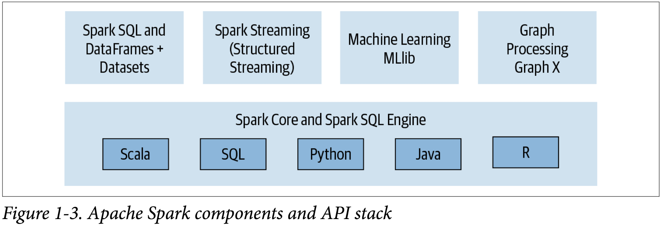
Modularity
Spark SQL, Spark Structured Streaming, Spark MLlib, and GraphX
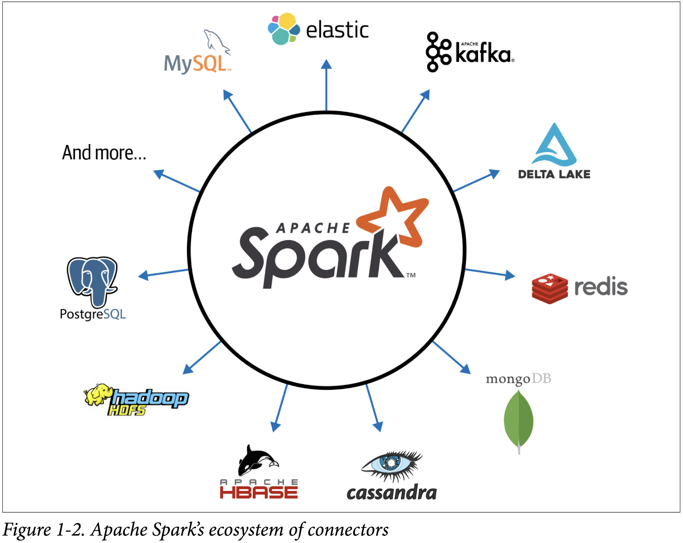
Extensibiltiy
Spark to read data stored in myriad sources—Apache Hadoop, Apache Cassandra, Apache HBase, MongoDB, Apache Hive, RDBMSs, and more—and process it all in memory. Spark’s DataFrameReaders and DataFrame Writers can also be extended to read data from other sources, such as Apache Kafka, Kinesis, Azure Storage, and Amazon S3, into its logical data abstraction, on which it can operate.
Spark Components
Apache Spark’s Distributed Execution
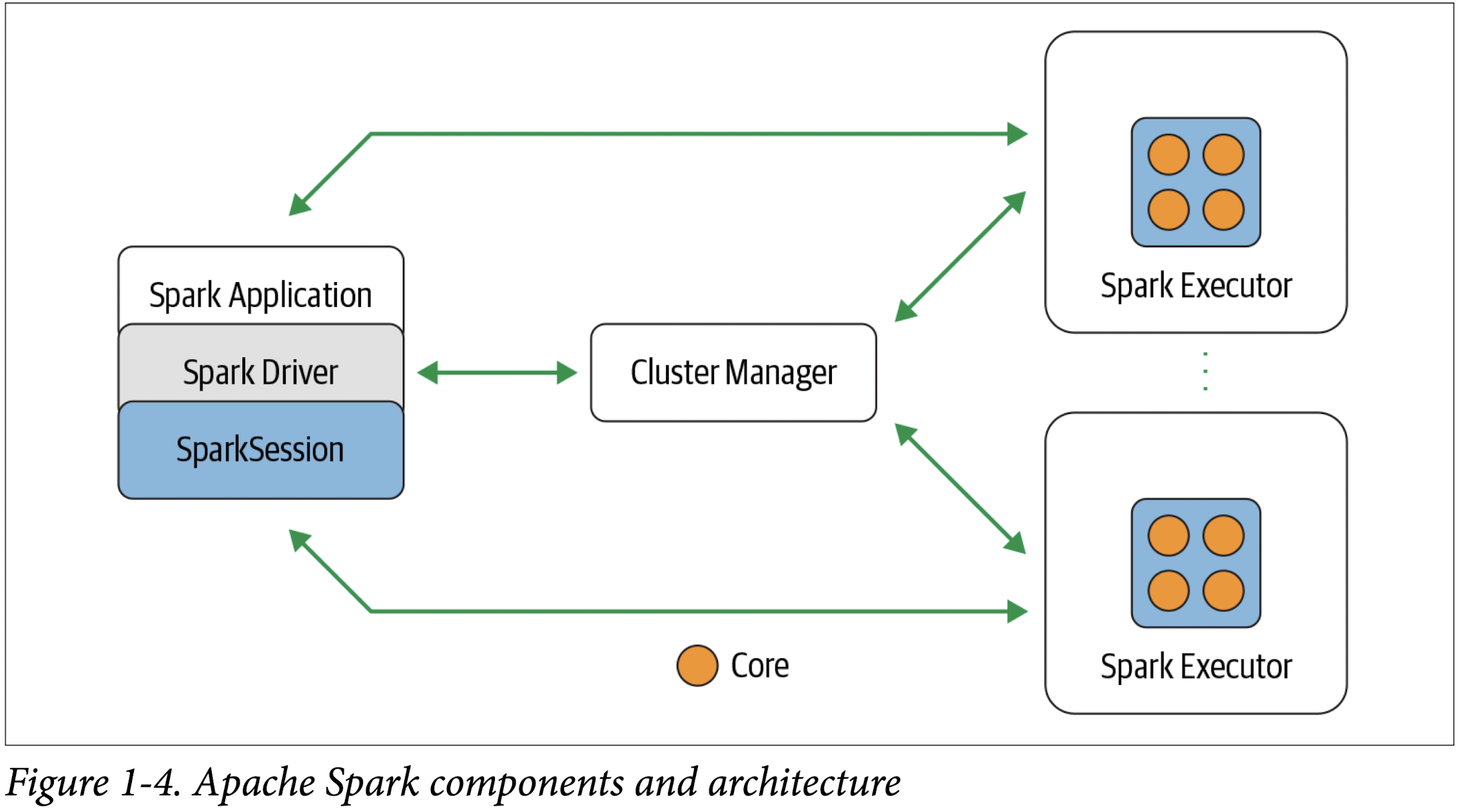
Spark driver
As the part of the Spark application responsible for instantiating a SparkSession, the Spark driver has multiple roles: it communicates with the cluster manager; it requests resources (CPU, memory, etc.) from the cluster manager for Spark’s executors (JVMs); and it transforms all the Spark operations into DAG computations, schedules them, and distributes their execution as tasks across the Spark executors. Once the resources are allocated, it communicates directly with the executors.
SparkSession
In Spark 2.0, the SparkSession became a unified conduit to all Spark operations and data. Not only did it subsume previous entry points to Spark like the SparkContext, SQLContext, HiveContext, SparkConf, and StreamingContext, but it also made working with Spark simpler and easier
Cluster manager
The cluster manager is responsible for managing and allocating resources for the cluster of nodes on which your Spark application runs. Currently, Spark supports four cluster managers: the built-in standalone cluster manager, Apache Hadoop YARN, Apache Mesos, and Kubernetes.
Spark executor
A Spark executor runs on each worker node in the cluster. The executors communicate with the driver program and are responsible for executing tasks on the workers. In most deployments modes, only a single executor runs per node.
Deployment methods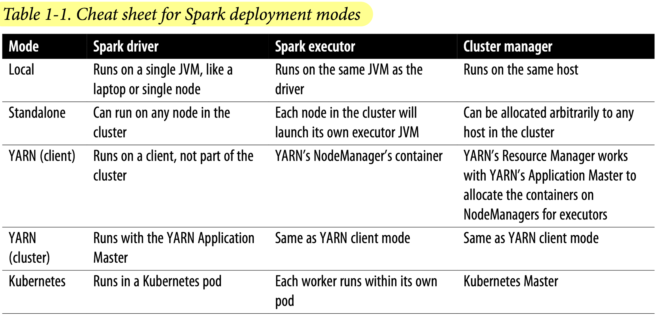
Distributed data and partitions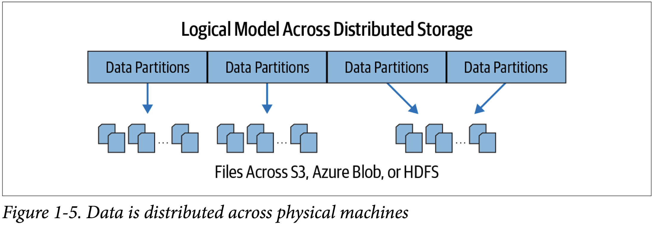
Spark Shell
1 | scala> val strings = spark.read.text("spark-3.2.1-bin-hadoop3.2/README.md") |
1 | strings = spark.read.text("spark-3.2.1-bin-hadoop3.2/README.md") |
1 | strings.show(10, truncate=True) |
Spark Application
Spark Application Concepts
Application
- A user program built on Spark using its APIs. It consists of a driver program and executors on the cluster.
SparkSession
- An object that provides a point of entry to interact with underlying Spark functionality and allows programming Spark with its APIs. In an interactive Spark shell, the Spark driver instantiates a SparkSession for you, while in a Spark application, you create a SparkSession object yourself.
Job
- A parallel computation consisting of multiple tasks that gets spawned in response to a Spark action (e.g.,
save(),collect()).
Stage
- Each job gets divided into smaller sets of tasks called stages that depend on each other.
Task
- A single unit of work or execution that will be sent to a Spark executor.
Spark Application and SparkSession
At the core of every Spark application is the Spark driver program, which creates a SparkSession object. When you’re working with a Spark shell, the driver is part of the shell and the SparkSession object (accessible via the variable spark) is created for you, as you saw in the earlier examples when you launched the shells.
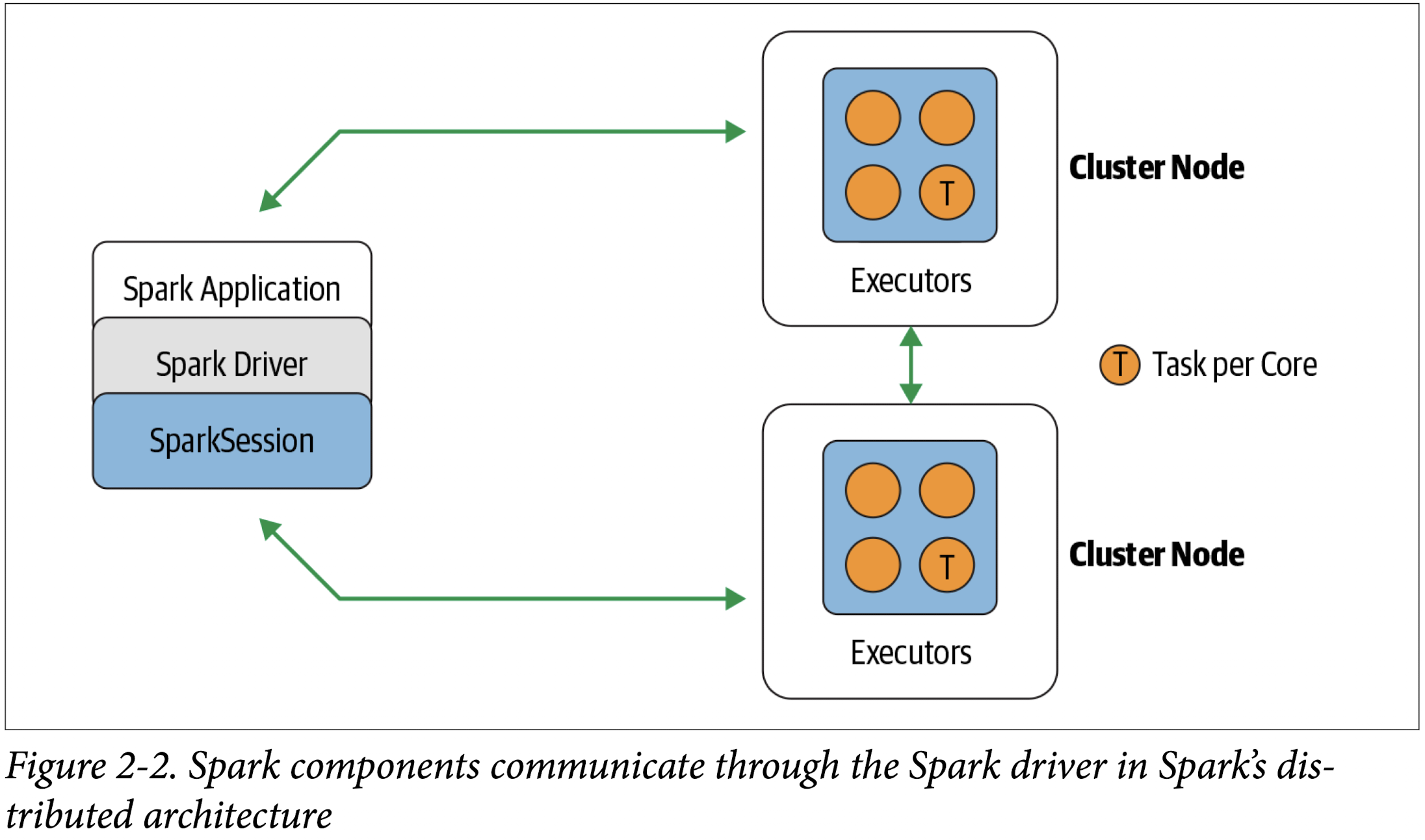
In those examples, because you launched the Spark shell locally on your laptop, all the operations ran locally, in a single JVM. But you can just as easily launch a Spark shell to analyze data in parallel on a cluster as in local mode. The commands spark-shell –help or pyspark –help will show you how to connect to the Spark cluster man‐ ager. Figure 2-2 shows how Spark executes on a cluster once you’ve done this.
Once you have a SparkSession, you can program Spark using the APIs to perform Spark operations.
Spark Jobs
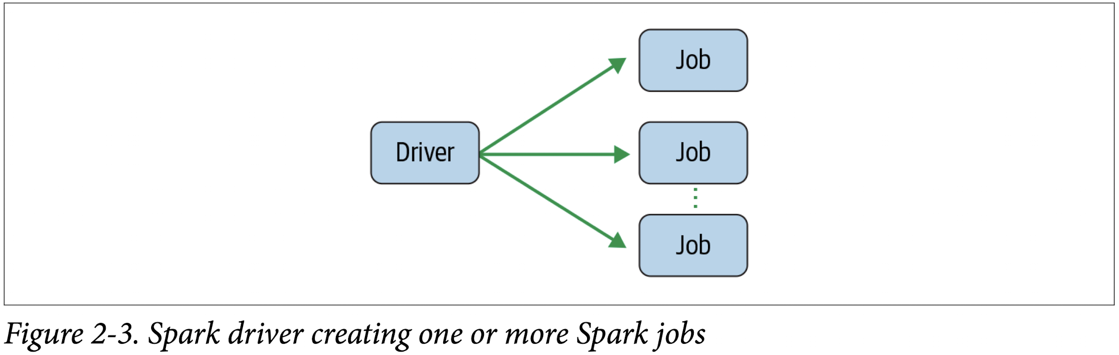
During interactive sessions with Spark shells, the driver converts your Spark applica‐ tion into one or more Spark jobs (Figure 2-3). It then transforms each job into a DAG. This, in essence, is Spark’s execution plan, where each node within a DAG could be a single or multiple Spark stages.
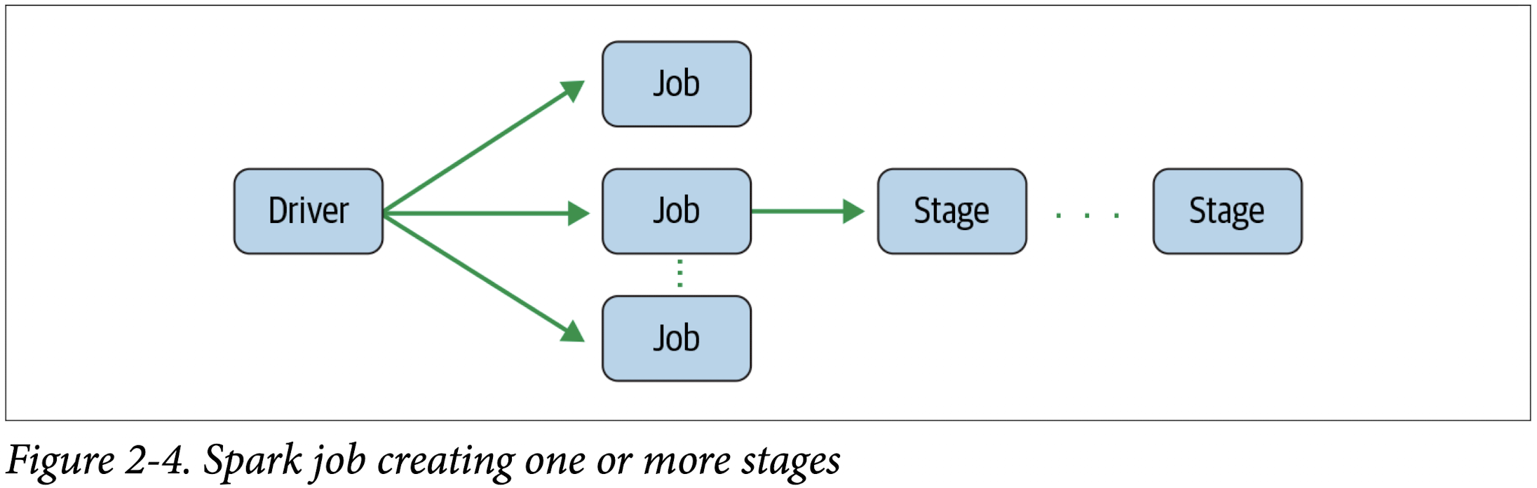
Spark Stage
As part of the DAG nodes, stages are created based on what operations can be per‐ formed serially or in parallel (Figure 2-4). Not all Spark operations can happen in a single stage, so they may be divided into multiple stages. Often stages are delineated on the operator’s computation boundaries, where they dictate data transfer among Spark executors.
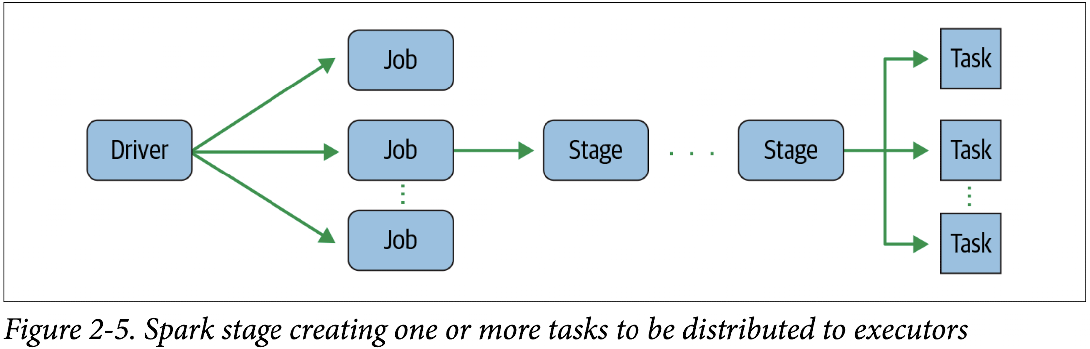
Spark Tasks
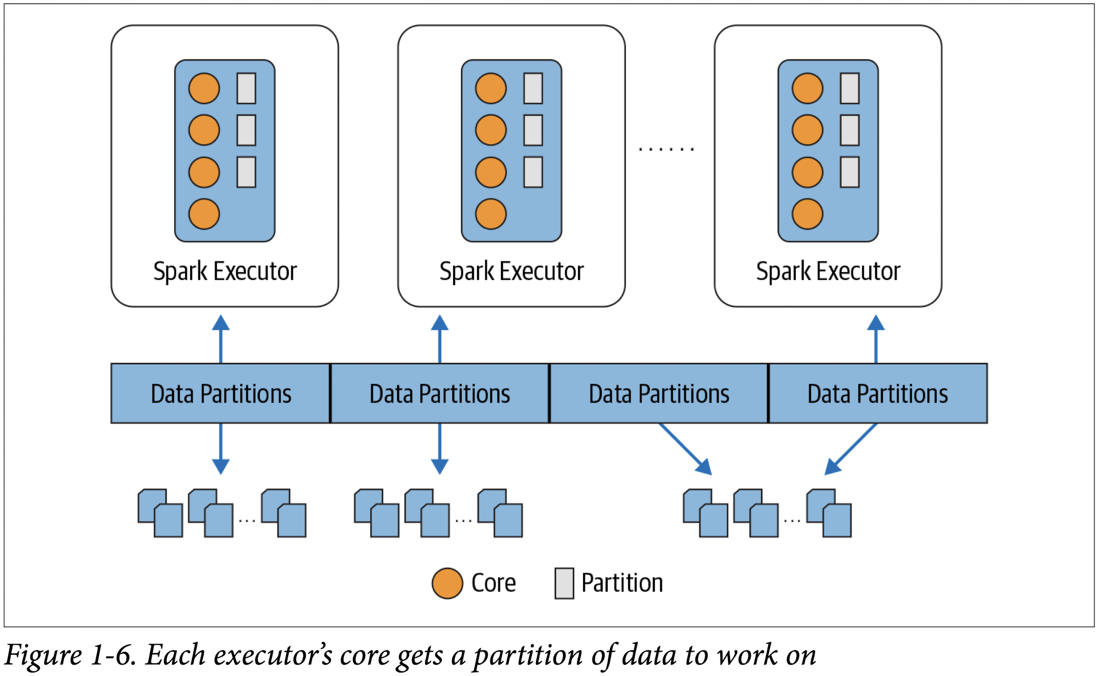
Each stage is comprised of Spark tasks (a unit of execution), which are then federated across each Spark executor; each task maps to a single core and works on a single par‐ tition of data (Figure 2-5). As such, an executor with 16 cores can have 16 or more tasks working on 16 or more partitions in parallel, making the execution of Spark’s tasks exceedingly parallel!
Transformations, Actions, and Lazy Evaluation
Spark operations on distributed data can be classified into two types: transformations and actions. Transformations, as the name suggests, transform a Spark DataFrame into a new DataFrame without altering the original data, giving it the property of immutability. Put another way, an operation such as select() or filter() will not change the original DataFrame; instead, it will return the transformed results of the operation as a new DataFrame.
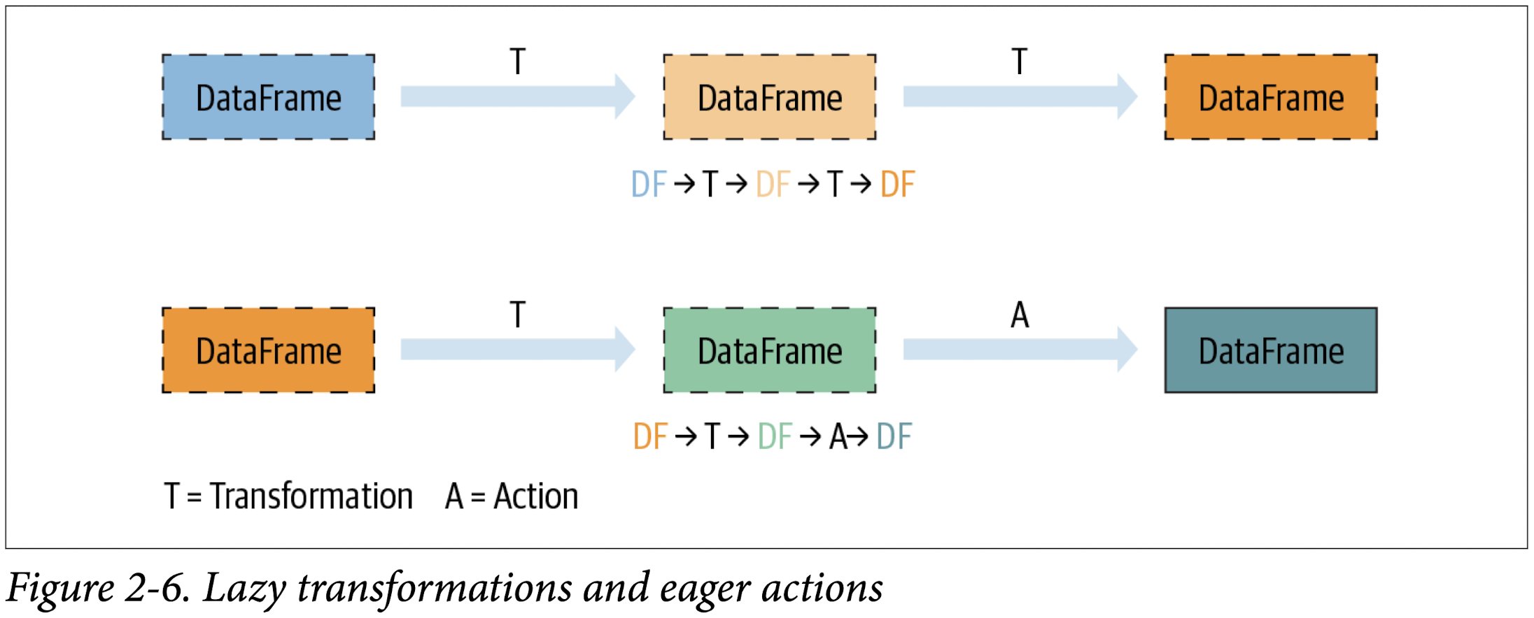
All transformations are evaluated lazily. That is, their results are not computed immediately, but they are recorded or remembered as a lineage. A recorded lineage allows Spark, at a later time in its execution plan, to rearrange certain transformations, coalesce them, or optimize transformations into stages for more efficient execution. Lazy evaluation is Spark’s strategy for delaying execution until an action is invoked or data is “touched” (read from or written to disk).
An action triggers the lazy evaluation of all the recorded transformations. In
Figure 2-6, all transformations T are recorded until the action A is invoked. Each transformation T produces a new DataFrame.
While lazy evaluation allows Spark to optimize your queries by peeking into your chained transformations, lineage and data immutability provide fault tolerance. Because Spark records each transformation in its lineage and the DataFrames are immutable between transformations, it can reproduce its original state by simply replaying the recorded lineage, giving it resiliency in the event of failures.
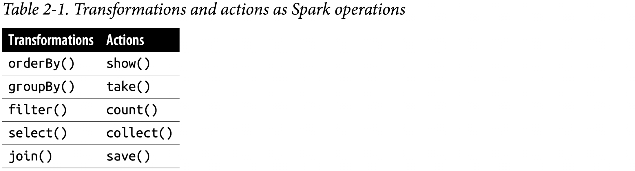
Table 2-1 lists some examples of transformations and actions.
Narrow and Wide Transformations
As noted, transformations are operations that Spark evaluates lazily. A huge advantage of the lazy evaluation scheme is that Spark can inspect your computational query and ascertain how it can optimize it. This optimization can be done by either joining or pipelining some operations and assigning them to a stage, or breaking them into stages by determining which operations require a shuffle or exchange of data across clusters.
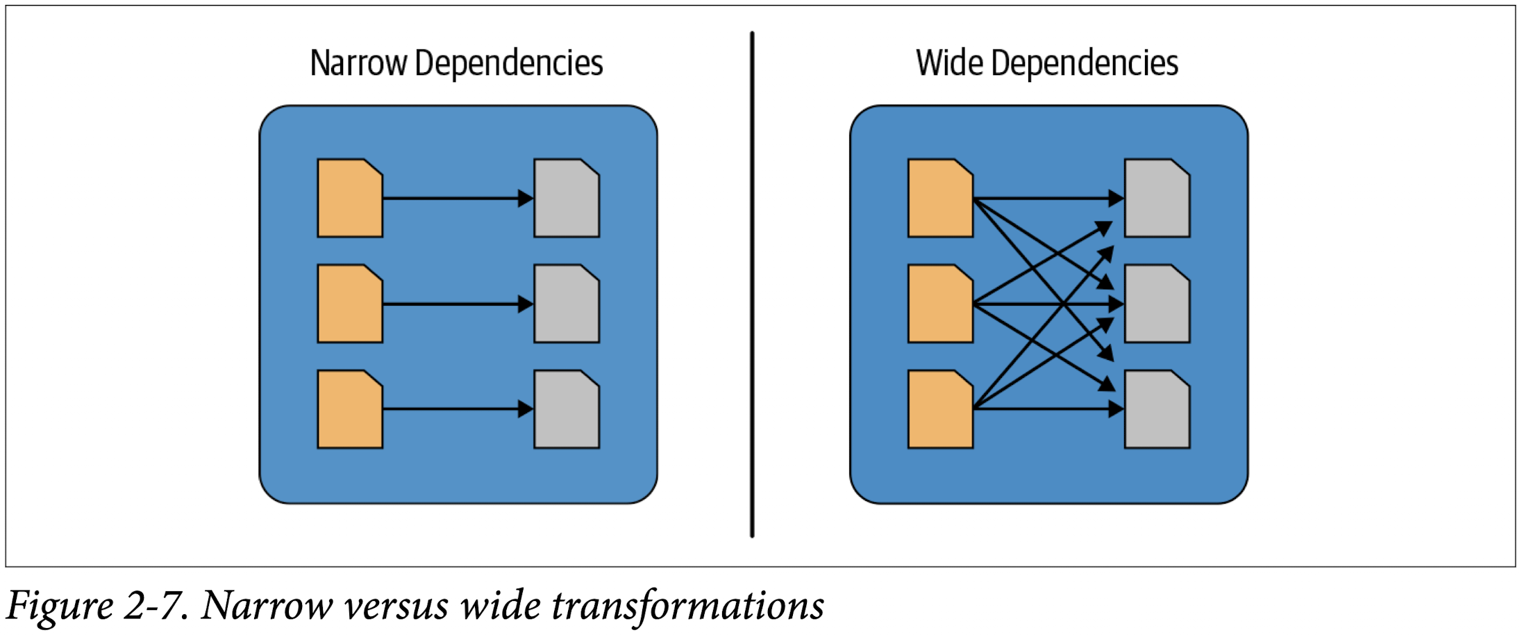
Transformations can be classified as having either narrow dependencies or wide dependencies. Any transformation where a single output partition can be computed from a single input partition is a narrow transformation. For example, in the previous code snippet,filter() and contains() represent narrow transformations because they can operate on a single partition and produce the resulting output partition without any exchange of data.
However, groupBy() or orderBy() instruct Spark to perform wide transformations, where data from other partitions is read in, combined, and written to disk. Since each partition will have its own count of the word that contains the “Spark” word in its row of data, a count (groupBy()) will force a shuffle of data from each of the executor’s partitions across the cluster. In this transformation, orderBy() requires output from other partitions to compute the final aggregation.
Figure 2-7 illustrates the two types of dependencies.
The Spark UI
Spark includes a graphical user interface that you can use to inspect or monitor Spark applications in their various stages of decomposition—that is jobs, stages, and tasks. Depending on how Spark is deployed, the driver launches a web UI, running by default on port 4040, where you can view metrics and details such as:
- A list of scheduler stages and tasks
- A summary of RDD sizes and memory usage
- Information about the environment
- Information about the running executors
- All the Spark SQL queries
In local mode, you can access this interface at http://<localhost>:4040 in a web browser.
Counting M&Ms for the Cookie Monster
Set environment variables
env– The command allows you to run another program in a custom environment without modifying the current one. When used without an argument it will print a list of the current environment variables.printenv– The command prints all or the specified environment variables.set– The command sets or unsets shell variables. When used without an argument it will print a list of all variables including environment and shell variables, and shell functions.unset– The command deletes shell and environment variables.export– The command sets environment variables./etc/environment- Use this file to set up system-wide environment variables./etc/profile- Variables set in this file are loaded whenever a bash login shell is entered. ```Per-user shell specific configuration files. For example, if you are using Bash, you can declare the variables in the
~/.bashrc:
Set your SPARK_HOME environment variable to the root-level directory where you installed Spark on your local machine.
1 | ➜ spark-3.2.1-bin-hadoop3.2 pwd |
1 | ➜ spark-3.2.1-bin-hadoop3.2 echo 'export SPARK_HOME="/Users/zacks/Git/Data Science Projects/spark-3.2.1-bin-hadoop3.2"' >> ~/.zshrc |
Review ~/.zshrc
1 | ➜ spark-3.2.1-bin-hadoop3.2 tail -1 ~/.zshrc |
To avoid having verbose INFO messages printed to the console, copy the log4j.properties.template file to log4j.properties and set log4j.rootCategory=WARN in the conf/log4j.properties file.
Content in log4j.properties.template
1 | ➜ spark-3.2.1-bin-hadoop3.2 cat conf/log4j.properties.template |
1 | ➜ spark-3.2.1-bin-hadoop3.2 cp conf/log4j.properties.template conf/log4j.properties |
After edit log4j.rootCategory in log4j.properties
1 | ➜ spark-3.2.1-bin-hadoop3.2 cat conf/log4j.properties | grep log4j.rootCategory |
Spark Job
Under LearningSparkV2/chapter2/py/src
1 | ➜ src git:(dev) ✗ source ~/.zshrc |
Output:
1st table: head of df
2nd table: sum Count group by State, Color
3rd table: sum Count group by State, Color where Color = 'CA'
1 | WARNING: An illegal reflective access operation has occurred |
Spark’s Structured APIs
Spark: What’s Underneath an RDD?
The RDD is the most basic abstraction in Spark. There are three vital characteristics associated with an RDD:
- Dependencies
- Partitions (with some locality information)
- Compute function: Partition =>
Iterator[T]
All three are integral to the simple RDD programming API model upon which all higher-level functionality is constructed. First, a list of dependencies that instructs Spark how an RDD is constructed with its inputs is required. When necessary to reproduce results, Spark can recreate an RDD from these dependencies and replicate operations on it. This characteristic gives RDDs resiliency.
Second, partitions provide Spark the ability to split the work to parallelize computation on partitions across executors. In some cases—for example, reading from HDFS—Spark will use locality information to send work to executors close to the data. That way less data is transmitted over the network.
And finally, an RDD has a compute function that produces an Iterator[T] for the data that will be stored in the RDD.
Structuring Spark
Key Metrics and Benefits
Structure yields a number of benefits, including better performance and space efficiency across Spark components. We will explore these benefits further when we talk about the use of the DataFrame and Dataset APIs shortly, but for now we’ll concentrate on the other advantages: expressivity, simplicity, composability, and uniformity.
Let’s demonstrate expressivity and composability first, with a simple code snippet. In the following example, we want to aggregate all the ages for each name, group by name, and then average the ages—a common pattern in data analysis and discovery. If we were to use the low-level RDD API for this, the code would look as follows:
1 | # In Python |
No one would dispute that this code, which tells Spark how to aggregate keys and compute averages with a string of lambda functions, is cryptic and hard to read. In other words, the code is instructing Spark how to compute the query. It’s completely opaque to Spark, because it doesn’t communicate the intention. Furthermore, the equivalent RDD code in Scala would look very different from the Python code shown here.
By contrast, what if we were to express the same query with high-level DSL operators and the DataFrame API, thereby instructing Spark what to do? Have a look:
1 | # In Python |
The DataFrame API
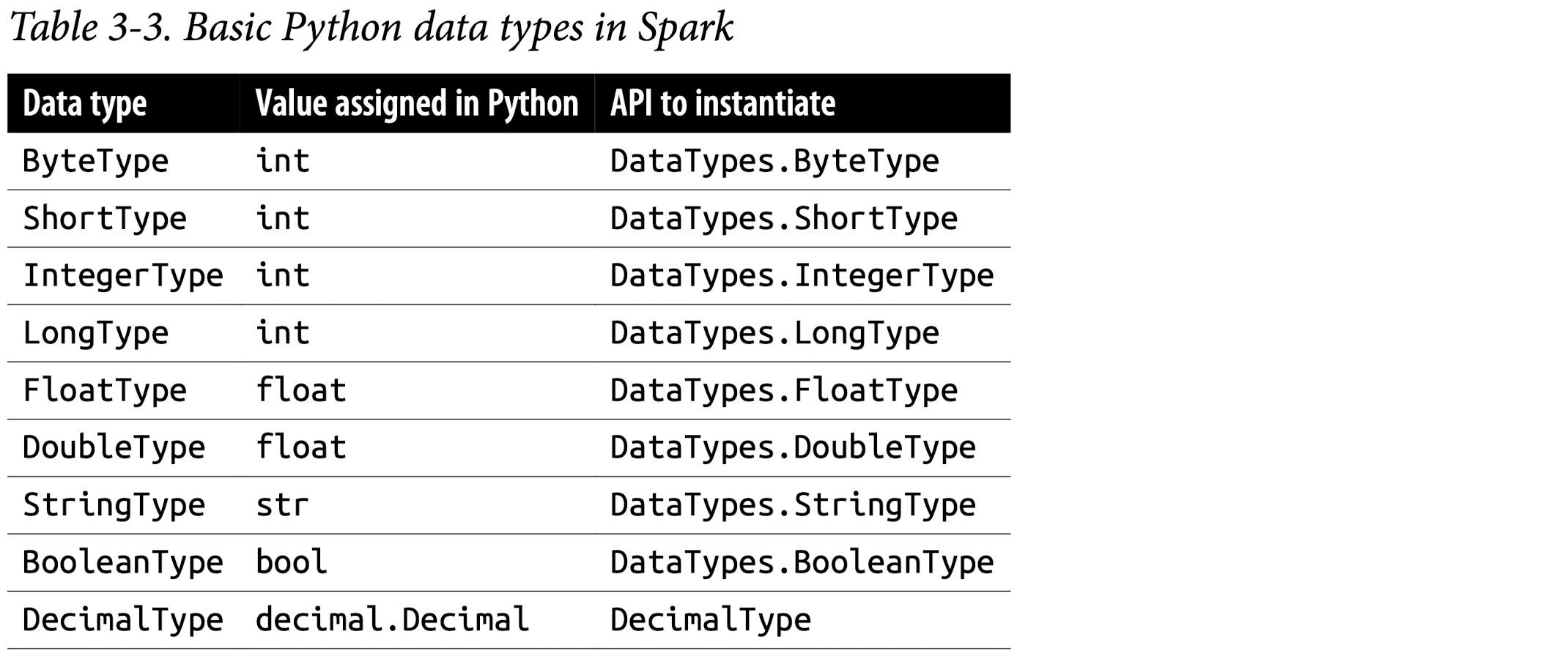
Spark’s Basic Data Types
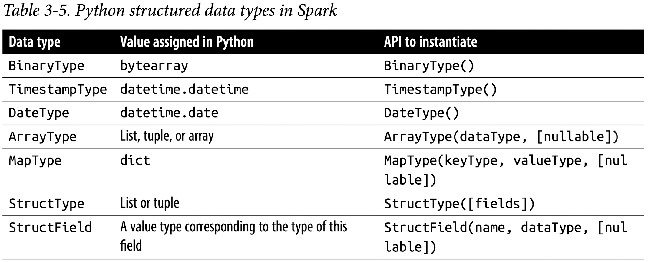
Spark’s Structured and Complex Data Types
Schemas and Creating DataFrames
A schema in Spark defines the column names and associated data types for a DataFrame.
Defining a schema up front as opposed to taking a schema-on-read approach offers three benefits:
- You relieve Spark from the onus of inferring data types.
- You prevent Spark from creating a separate job just to read a large portion of your file to ascertain the schema, which for a large data file can be expensive and time-consuming.
- You can detect errors early if data doesn’t match the schema.
So, we encourage you to always define your schema up front whenever you want to read a large file from a data source.
Two ways to define a schema
Spark allows you to define a schema in two ways. One is to define it programmatically, and the other is to employ a Data Definition Language (DDL) string, which is much simpler and easier to read.
To define a schema programmatically for a DataFrame with three named columns, author, title, and pages, you can use the Spark DataFrame API. For example:
1 | # In Python |
Defining the same schema using DDL is much simpler:
1 | # In Python |
You can choose whichever way you like to define a schema. For many examples, we will use both:
1 | # define schema by using Spark DataFrame API |
1 | # define schema by using Definition Language (DDL) |
Columns and Expressions
Named columns in DataFrames are conceptually similar to named columns in pandas or R DataFrames or in an RDBMS table: they describe a type of field. You can list all the columns by their names, and you can perform operations on their values using relational or computational expressions. In Spark’s supported languages, columns are objects with public methods (represented by the Column type).
You can also use logical or mathematical expressions on columns. For example, you could create a simple expression using expr("columnName * 5") or (expr("columnName - 5") > col(anothercolumnName)), where columnName is a Spark type (integer, string, etc.). expr() is part of the pyspark.sql.functions (Python) and org.apache.spark.sql.functions (Scala) packages. Like any other function in those packages, expr() takes arguments that Spark will parse as an expression, computing the result.
Scala, Java, and Python all have public methods associated with columns. You’ll note that the Spark documentation refers to both col and Column. Column is the name of the object, while col() is a standard built-in function that returns a Column.
Rows
A row in Spark is a generic Row object, containing one or more columns. Each column may be of the same data type (e.g., integer or string), or they can have different types (integer, string, map, array, etc.). Because Row is an object in Spark and an ordered collection of fields, you can instantiate a Row in each of Spark’s supported languages and access its fields by an index starting at 0:
1 | from pyspark.sql import Row |
Row objects can be used to create DataFrames if you need them for quick interactivity and exploration:
1 | rows = [Row("Matei Zaharia", "CA"), Row("Reynold Xin", "CA")] |
Common DataFrame Operations
To perform common data operations on DataFrames, you’ll first need to load a Data‐ Frame from a data source that holds your structured data. Spark provides an inter‐ face, DataFrameReader, that enables you to read data into a DataFrame from myriad data sources in formats such as JSON, CSV, Parquet, Text, Avro, ORC, etc. Likewise, to write a DataFrame back to a data source in a particular format, Spark uses DataFrameWriter.
Using DataFrameReader and DataFrameWriter
By defining a schema and use DataFrameReader class and its methods to tell Spark what to do, it’s more efficient to define a schema than have Spark infer it.
inferSchema
If you don’t want to specify the schema, Spark can infer schema from a sample at a lesser cost. For example, you can use the samplingRatio option(under chapter3 directory):
1 | sampleDF = (spark |
The following example shows how to read DataFrame with a schema:
1 | from pyspark.sql.types import * |
The spark.read.csv() function reads in the CSV file and returns a DataFrame of rows and named columns with the types dictated in the schema.
To write the DataFrame into an external data source in your format of choice, you can use the DataFrameWriter interface. Like DataFrameReader, it supports multiple data sources. Parquet, a popular columnar format, is the default format; it uses snappy compression to compress the data. If the DataFrame is written as Parquet, the schema is preserved as part of the Parquet metadata. In this case, subsequent reads back into a DataFrame do not require you to manually supply a schema.
Saving a DataFrame as a Parquet file or SQL table. A common data operation is to explore and transform your data, and then persist the DataFrame in Parquet format or save it as a SQL table. Persisting a transformed DataFrame is as easy as reading it. For exam‐ ple, to persist the DataFrame we were just working with as a file after reading it you would do the following:
1 | # In Python to save as Parquet files |
Alternatively, you can save it as a table, which registers metadata with the Hive meta-store (we will cover SQL managed and unmanaged tables, metastores, and Data-Frames in the next chapter):
1 | # In Python to save as a Hive metastore |
Transformations and actions
Projections and filters. A projection in relational parlance is a way to return only the rows matching a certain relational condition by using filters. In Spark, projections are done with the select() method, while filters can be expressed using the filter() or where() method. We can use this technique to examine specific aspects of our SF Fire Department data set:
1 | fire_parquet.select("IncidentNumber", "AvailableDtTm", "CallType") \ |
1 | +--------------+----------------------+-----------------------------+ |
What if we want to know how many distinct CallTypes were recorded as the causes of the fire calls? These simple and expressive queries do the job:
1 | (fire_parquet |
1 | +-----------------+ |
We can list the distinct call types in the data set using these queries:
1 | # In Python, filter for only distinct non-null CallTypes from all the rows |
Renaming, adding, and dropping columns. Sometimes you want to rename particular columns for reasons of style or convention, and at other times for readability or brevity. The original column names in the SF Fire Department data set had spaces in them. For example, the column name IncidentNumber was Incident Number. Spaces in column names can be problematic, especially when you want to write or save a DataFrame as a Parquet file (which prohibits this).
By specifying the desired column names in the schema with StructField, as we did, we effectively changed all names in the resulting DataFrame.
Alternatively, you could selectively rename columns with the withColumnRenamed() method. For instance, let’s change the name of our Delay column to ResponseDelayedinMins and take a look at the response times that were longer than five minutes:
1 | # create a new dataframe new_fire_parquet from fire_parquet |
1 | +---------------------+ |
Because DataFrame transformations are immutable, when we rename a column using
withColumnRenamed()we get a new DataFrame while retaining the original with the old column name.
Modifying the contents of a column or its type are common operations during data exploration. In some cases the data is raw or dirty, or its types are not amenable to