Python Data Science
Python Tutorial
Regular Expression
Random
Introduction
Python has a built-in module that you can use to make random numbers.
The random module has a set of methods:
| Method | Description |
|---|---|
| seed() | Initialize the random number generator |
| getstate() | Returns the current internal state of the random number generator |
| setstate() | Restores the internal state of the random number generator |
| getrandbits() | Returns a number representing the random bits |
| randrange() | Returns a random number between the given range |
| randint() | Returns a random number between the given range |
| choice() | Returns a random element from the given sequence |
| choices() | Returns a list with a random selection from the given sequence |
| shuffle() | Takes a sequence and returns the sequence in a random order |
| sample() | Returns a given sample of a sequence |
| random() | Returns a random float number between 0 and 1 |
| uniform() | Returns a random float number between two given parameters |
| triangular() | Returns a random float number between two given parameters, you can also set a mode parameter to specify the midpoint between the two other parameters |
| betavariate() | Returns a random float number between 0 and 1 based on the Beta distribution (used in statistics) |
| expovariate() | Returns a random float number based on the Exponential distribution (used in statistics) |
| gammavariate() | Returns a random float number based on the Gamma distribution (used in statistics) |
| gauss() | Returns a random float number based on the Gaussian distribution (used in probability theories) |
| lognormvariate() | Returns a random float number based on a log-normal distribution (used in probability theories) |
| normalvariate() | Returns a random float number based on the normal distribution (used in probability theories) |
| vonmisesvariate() | Returns a random float number based on the von Mises distribution (used in directional statistics) |
| paretovariate() | Returns a random float number based on the Pareto distribution (used in probability theories) |
| weibullvariate() | Returns a random float number based on the Weibull distribution (used in statistics) |
seed()
Definition and Usage
The seed() method is used to initialize the random number generator.
The random number generator needs a number to start with (a seed value), to be able to generate a random number.
By default the random number generator uses the current system time.
Use the seed() method to customize the start number of the random number generator.
Syntax
1 | random.seed(a, version) |
| Parameter | Description |
|---|---|
| a | Optional. The seed value needed to generate a random number. If it is an integer it is used directly, if not it has to be converted into an integer. Default value is None, and if None, the generator uses the current system time. |
| version | An integer specifying how to convert the a
parameter into a integer.Default value is 2 |
Note: If you use the same seed value twice you will get the same random number twice. Setting a random seed is important for giving others an opportunity to reproduce the results of your experiment.
Example
1 | import random |
randint()
Definition and Usage
The randint() method returns an integer number selected element from the specified range.
Note: This method is an alias for random.randrange(start, stop+1).
Syntax
1 | random.randint(start, stop) |
Parameter Values
| Parameter | Description |
|---|---|
| start | Required. An integer specifying at which position to start inclusively. |
| stop | Required. An integer specifying at which position to end inclusively. |
Numpy Array
Numpy Org
NumPy Developer Documentation
NumPy User Guide
NumPy Reference
Numpy Quickstart tutorial
NumPy: the absolute basics for beginners
Introduction
In computer science, an array data structure, or simply an array, is a data structure consisting of a collection of the same type of elements (values or variables), each identified by at least one array index or key. An array is stored such that the position of each element can be computed from its index tuple by a mathematical formula. The simplest type of data structure is a linear array, also called one-dimensional array.
The array is a concept that similar to Matrix (mathematics). In mathematics, a matrix (plural matrices) is a rectangular array of numbers, symbols, or expressions, arranged in rows and columns. For example, the dimension of the matrix below is $2 × 3$ (read “two by three”), because there are two rows and three columns:
$$
\left[
\begin{matrix}
1 & 2 & 3 \
4 & 5 & 6 \
\end{matrix}
\right]
$$
The matrix always called a $m \times n \space matrix$. $m$ is the number of the rows; $n$ is the number of the columns. Therefore, the above sample is a two-dimensional array.
And in Numpy, dimensions are called axes. There is a little difference between mathematic matrix and computer science array. In mathematic matrix, the first index is 1. But in computer science, the first index is 0.
One-dimensional array
1D array has almost the same appearance as the list.
1 | import numpy as np |
1D array only has one axis, the row. And in the following sample, the length of axis = 0 is three since we have three elements.
1 | import numpy as np |
Two-dimensional array
2D array has two axes. In the following sample, the length of axis = 0 is three since we have three elements; the length of axis = 1 is two since we have two dimensions.
1 | import numpy as np |
Now we have an array a that has two axes.
| col 1 | col 2 | col 3 | |
|---|---|---|---|
| row 1 | 1 | 2 | 3 |
| row 2 | 4 | 5 | 6 |
1 | a[0] # the first row |
Three-dimensional array
3D array is hard to understand. But we can split it into 2 parts. And each part is a 2D array.
1 | import numpy as np |
Just imagine we have two tables, the 2D array, and we combine them together. Then we have a 3D array.
1 | a[0][0] # axis = 0, size = 0; axis = 1, size = 0 -> the first 2D array, the first row |
From the observation of the 3D array, we can know that in Numpy, the size is the value of a specific axis. For example, a[0][3] means in the first axis (axis = 0), the value is 0; in the second axis (axis = 1), the value is 3.
And whatever how many dimensions an array has, the first axis (axis = 0) should be overall view sight. And the last axis (axis = -1) should be the column. The last-second axis (axis = -2) is the row.
The difference between a Python list and a NumPy array
1 | height = [1.73, 1.68, 1.71, 1.89, 1.79] |
If you really need to figure out the product of height times weight, you have build your own code:
1 | height = [1.73, 1.68, 1.71, 1.89, 1.79] |
Or in an easier way:
1 | height = [1.73, 1.68, 1.71, 1.89, 1.79] |
However, the code is not concise enough. Additionally, you cannot use this method too many times. Therefore, let’s try the Numpy Array - also called ndarray(Numpy dtype array).
1 | import numpy as np |
What is an array?
An array is a central data structure of the NumPy library. An array is a grid of values and it contains information about the raw data, how to locate an element, and how to interpret an element. It has a grid of elements that can be indexed in various ways. The elements are all of the same type, referred to as the array dtype.
Create a basic array
np.array()
To create a NumPy array, you can use the function np.array().
All you need to do to create a simple array is pass a list to it. If you choose to, you can also specify the type of data in your list. You can find more information about data types here.
1 | import numpy as np |
Once you run the above code, the Numpy will initialize a row for array a. The row is a similar concept of dataframe, matrix, or database. In dataframe and database, we use column to store the same type of data. And we use row to store data from different individual.
For example, here is a sample dataframe of a table in a database.
| Name | Height | Age | Gender |
|---|---|---|---|
| Zack Fair | 1.85 | 23 | M |
| Cloud Strife | 1.73 | 21 | M |
Obviously, Name and Gender should be type string, Height should be type float, and Age should be type int. Every column stores the same type of the data
An array can be indexed by a tuple of nonnegative integers, by booleans, by another array, or by integers. The rank of the array is the number of dimensions. The shape of the array is a tuple of integers giving the size of the array along each dimension.
One way we can initialize NumPy arrays is from Python lists, using nested lists for two- or higher-dimensional data.
1 | import numpy as np |
| col 1 | col 2 | col 3 | |
|---|---|---|---|
| row 1 | 1 | 2 | 3 |
| row 2 | 4 | 5 | 6 |
| row 3 | 7 | 8 | 9 |
Sorting elements
np.sort()
Sorting an element is simple with np.sort(). You can specify the axis, kind, and order when you call the function.
1 | import numpy as np |
order: str or list of str, optional
When a is an array with fields defined, this argument specifies which fields to compare first, second, etc. A single field can be specified as a string, and not all fields need be specified, but unspecified fields will still be used, in the order in which they come up in the dtype, to break ties.
1 | import numpy as np |
In addition to sort, which returns a sorted copy of an array, you can use:
- argsort, which is an indirect sort along a specified axis,
- lexsort, which is an indirect stable sort on multiple keys,
- searchsorted, which will find elements in a sorted array, and
- partition, which is a partial sort.
np.concatenate()
You can concatenate arrays with np.concatenate().
1 | import numpy as np |
Attention: Do not use + in numpy. It is not the same as Python list.
1 | import numpy as np |
1 | import numpy as np |
Indexing, slicing, and filtering
Review the concepts of the axis if you cannot understand this chapter.
Indexing
Indexing 1D array.
1 | import numpy as np |
Indexing 2D array.
1 | a = np.array([[0, 1, 2, 3], [4, 5, 6, 7], [8, 9, 10, 11], [12, 13, 14, 15]]) |
Slicing
Slicing 1D array.
1 | import numpy as np |
Slicing 2D array.
1 | a = np.array([[0, 1, 2, 3], [4, 5, 6, 7], [8, 9, 10, 11], [12, 13, 14, 15]]) |
Filtering
Use the condition will only return the indices of the array.
1 | import numpy as np |
Use the indices for filtering the values you need.
1 | a[a < 5] |
You can also select, for example, numbers that are equal to or greater than 5, and use that condition to index an array.
1 | a[a >= 5] |
You can select elements that are divisible by 2:
1 | a[a%2 == 0] |
Or you can select elements that satisfy two conditions using the & and | operators:
1 | b = a[(a > 5) | (a == 5)] |
You can also use np.nonzero() to select elements or indices from an array.
1 | index = np.nonzero(a < 5) |
In this example, a tuple of arrays was returned: one for each dimension. The first array represents the row indices where these values are found, and the second array represents the column indices where the values are found.
If you want to generate a list of coordinates where the elements exist, you can zip the arrays, iterate over the list of coordinates, and print them. For example:
1 | list_of_coordinates = list(zip(index[0], index[1])) |
You can also use np.nonzero() to print the elements in an array that are less than 5 with:
1 | a[index] |
Create a bmi function.
1 | import numpy as np |
Numpy Statistics
Numpy Descriptive Statistics for Numerical Data
Measures of Location
Percentiles & Quartiles
1 | import numpy as np |
Arithmetic Mean
1 | import numpy as np |
Median
1 | import numpy as np |
Mode
1 | from scipy import stats |
Measures of Dispersion
Variance
1 | import numpy as np |
Standard Deviation
1 | import numpy as np |
Measures of Association
Correlation Coefficient
1 | import pandas as pd |

Correlation Coefficient in Dataframe
1 | np.corrcoef(df['Height(inches)'][:100], df['Weight(pounds)'][:100]) |
Correlation Coefficient in ndarray
1 | np_baseball = np.array(df) |
Pandas
DataFrames
Basic
- Sorting and subsetting
- Creating new columns
df: DataFrame Object
1 | print(df) |
Pandas Philosophy
There should be one – and preferably only one – obvious way to do it.
Sorting
1 | df.sort_values("column_name") |
Subsetting
1 | df["column_name"] |
New Columns
- Transforming, mutating, and feature engineering.
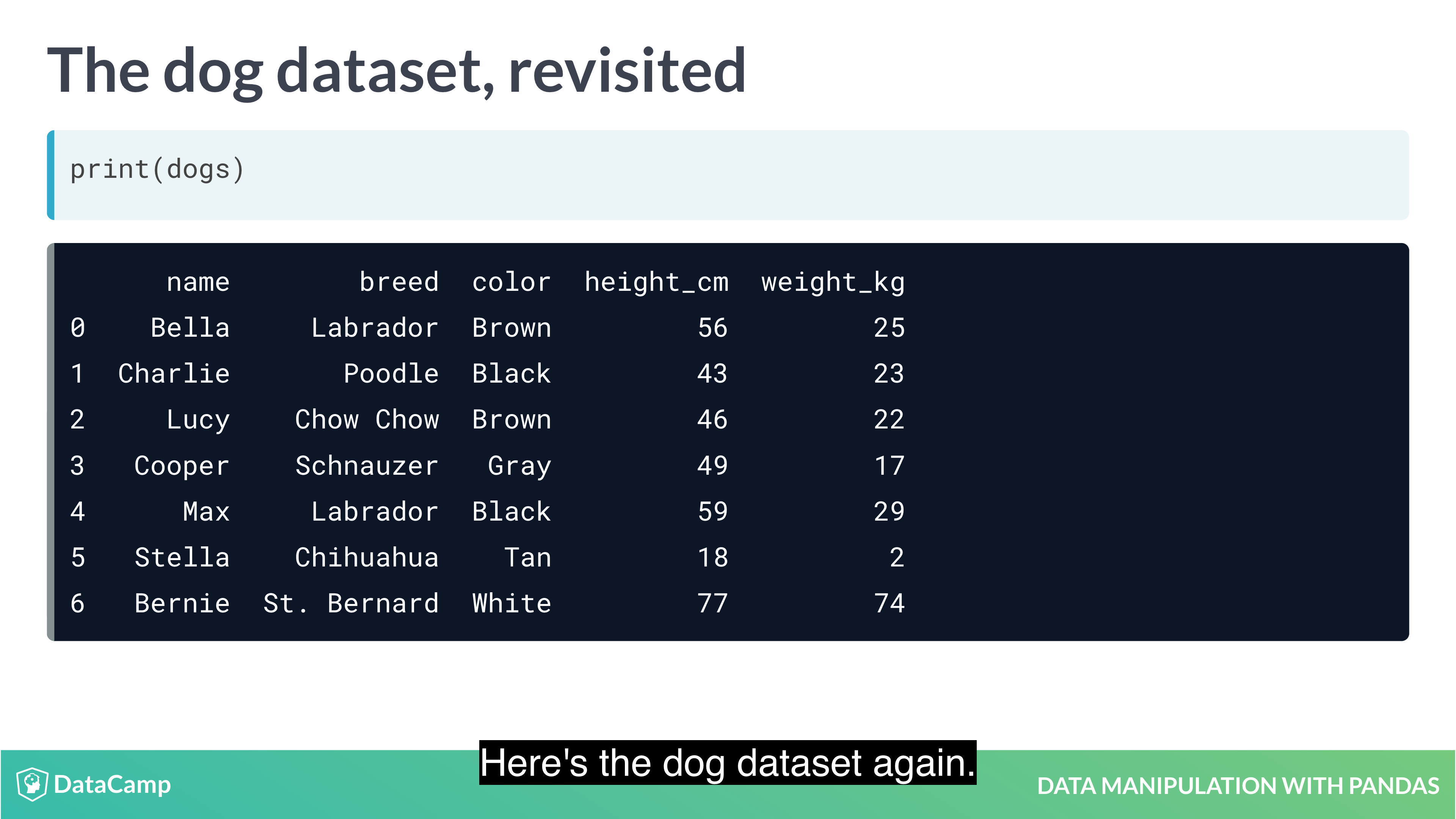
1 | dogs["bmi"] = dogs["wight_kg"] / dogs["height_m] ** 2 |
Aggregating Data
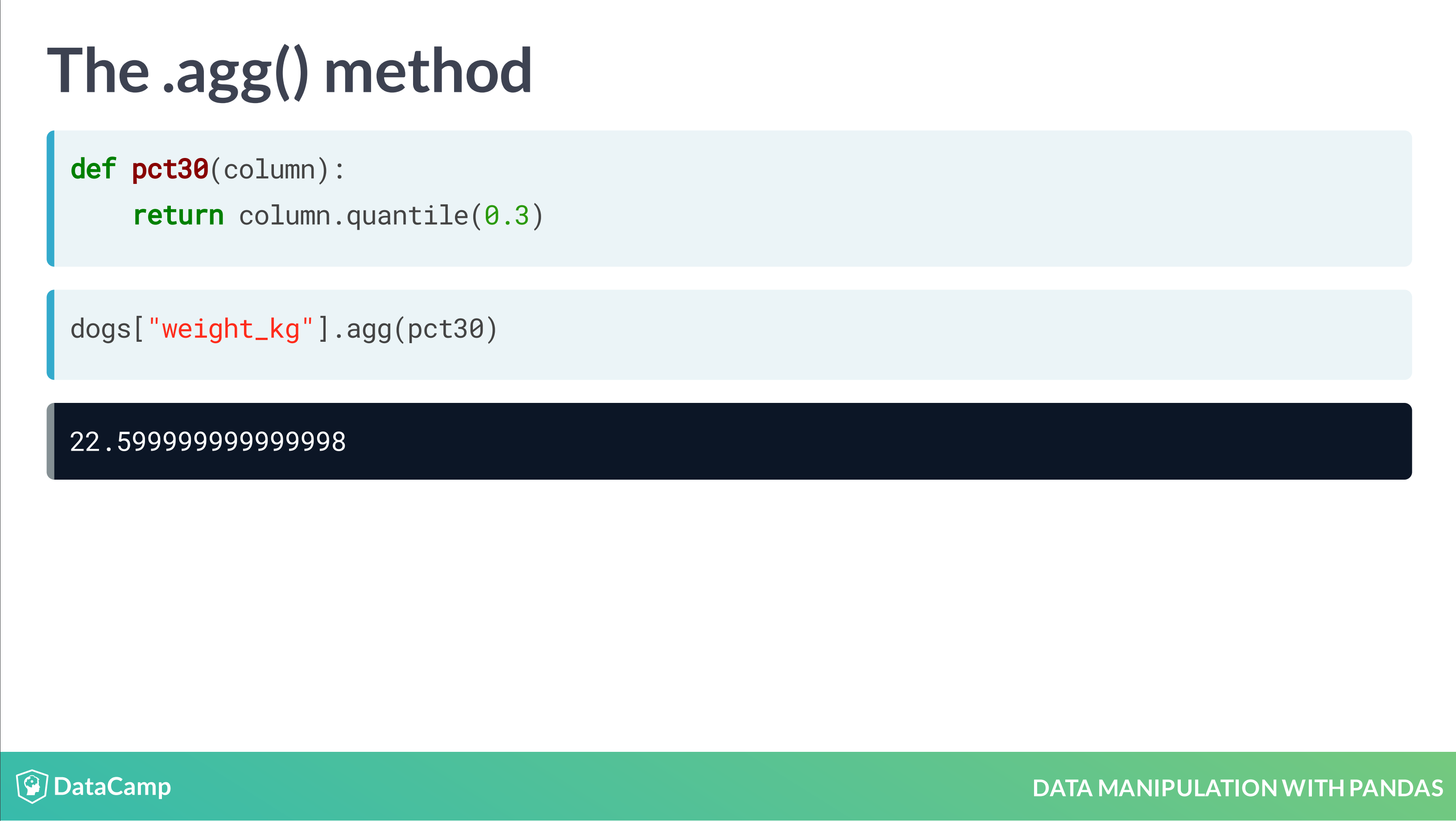
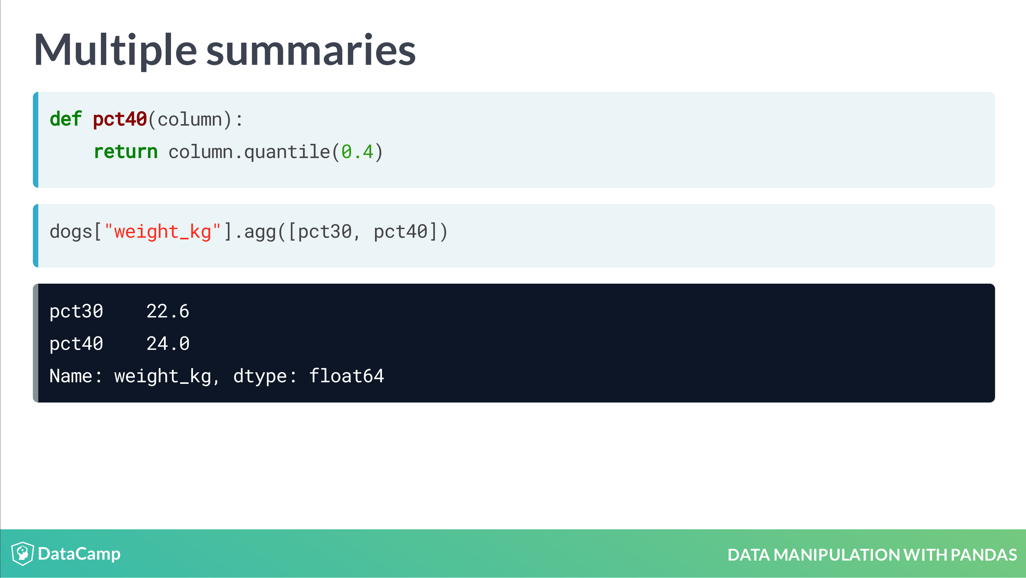
- Summary statistics
- Counting
- Grouped summary statistics
Summarizing Data
1 | df["column_name"].mean() |
Counting
1 | df.drop_duplicates(subset="column_names") |
Grouped Summary Statistics
Without Groupby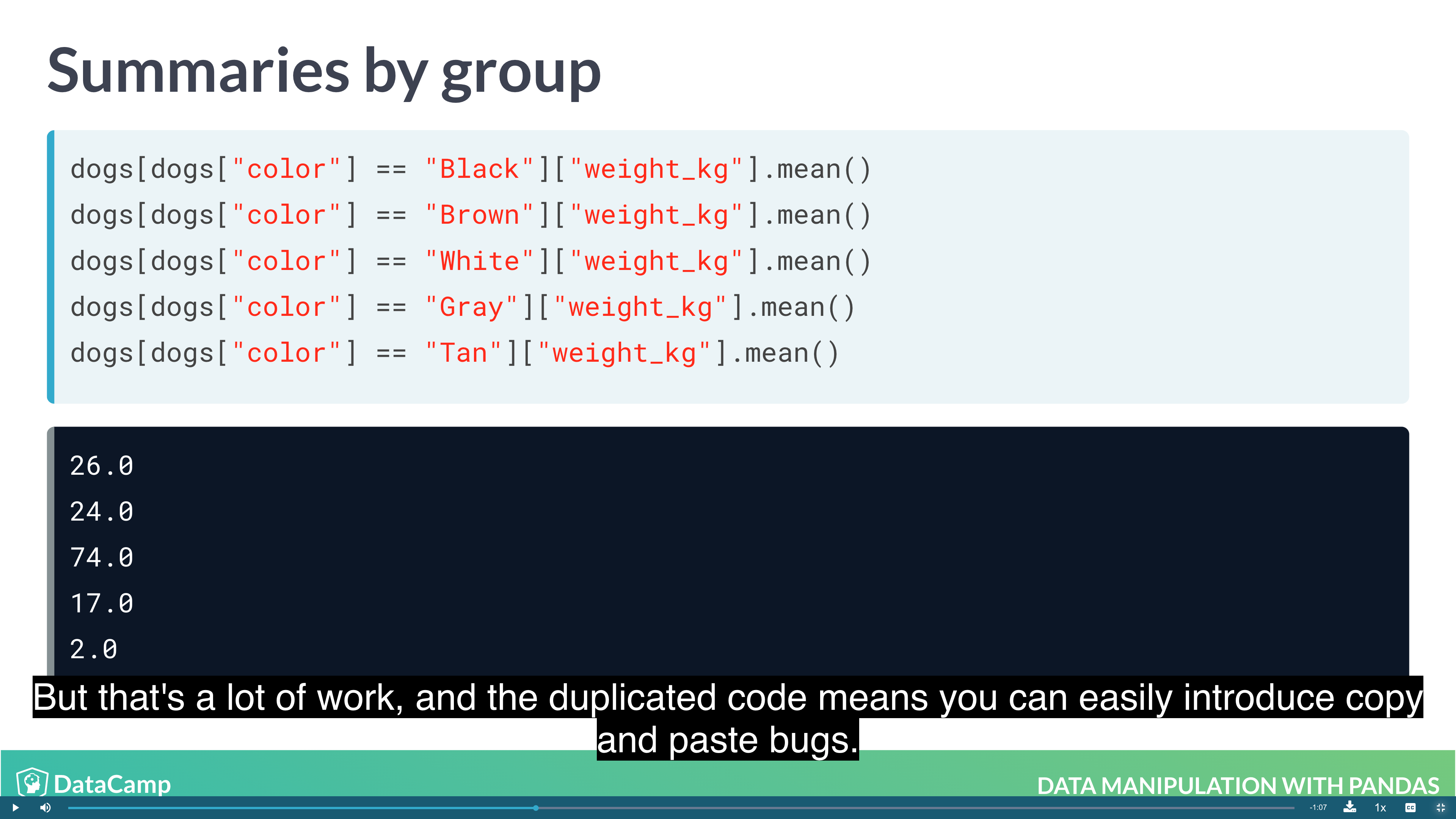
With Groupby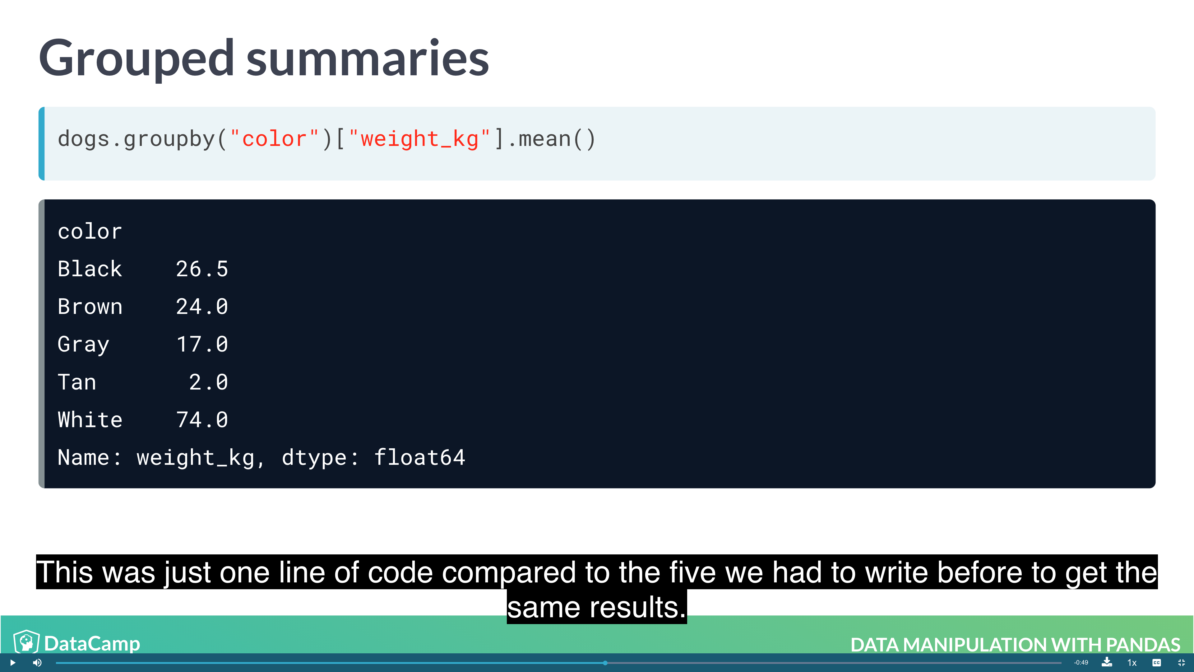
1 | dogs.groupby("color")["weight_kg"].mean() |
Multiple Grouped Summaries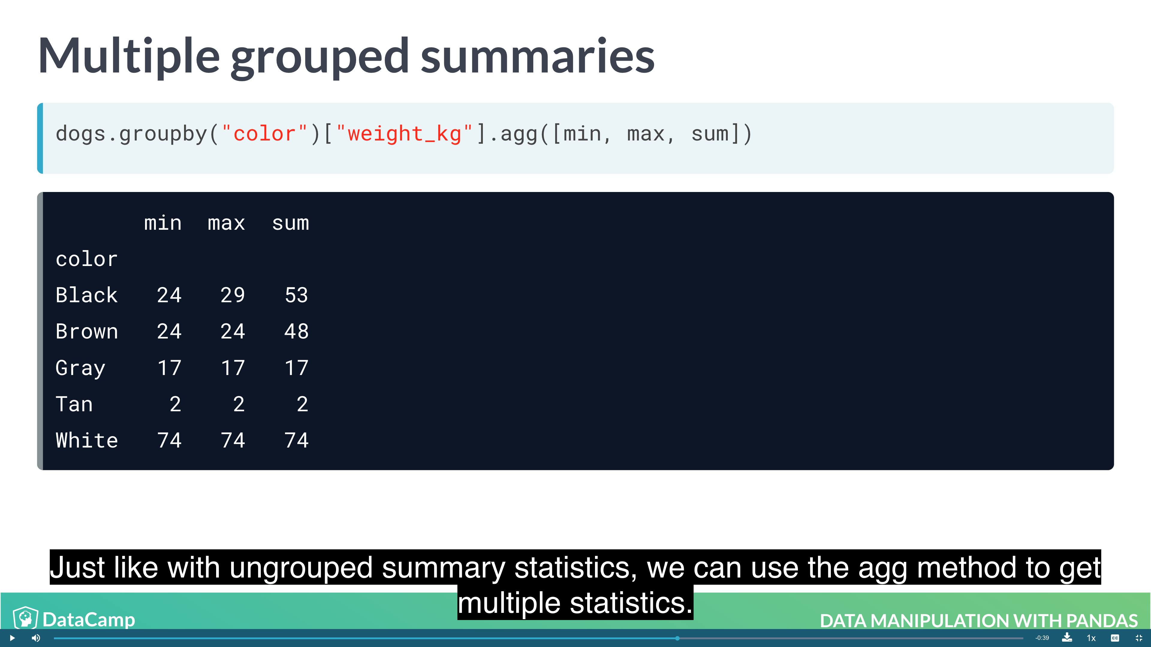
1 | dogs.groupby("color")["weight_kg"].agg([min, max, sum]) |
Grouping by multiple variables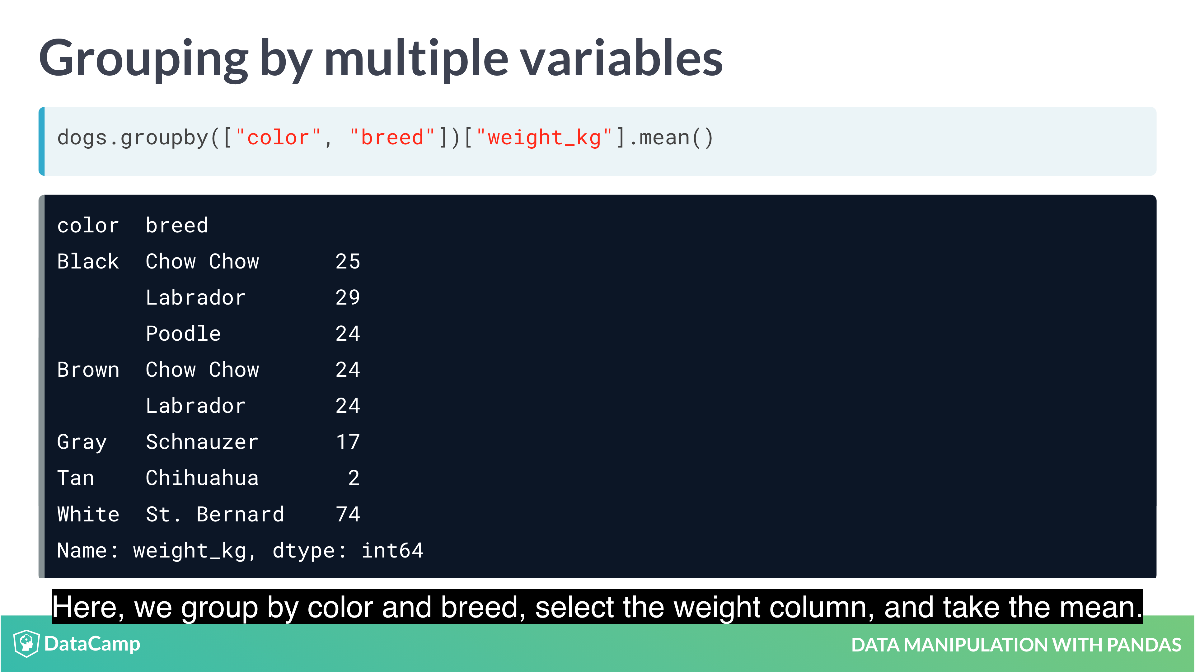
1 | dogs.groupby(["color", "breed"])["weight_kg"].mean() |
Many groups, many summaries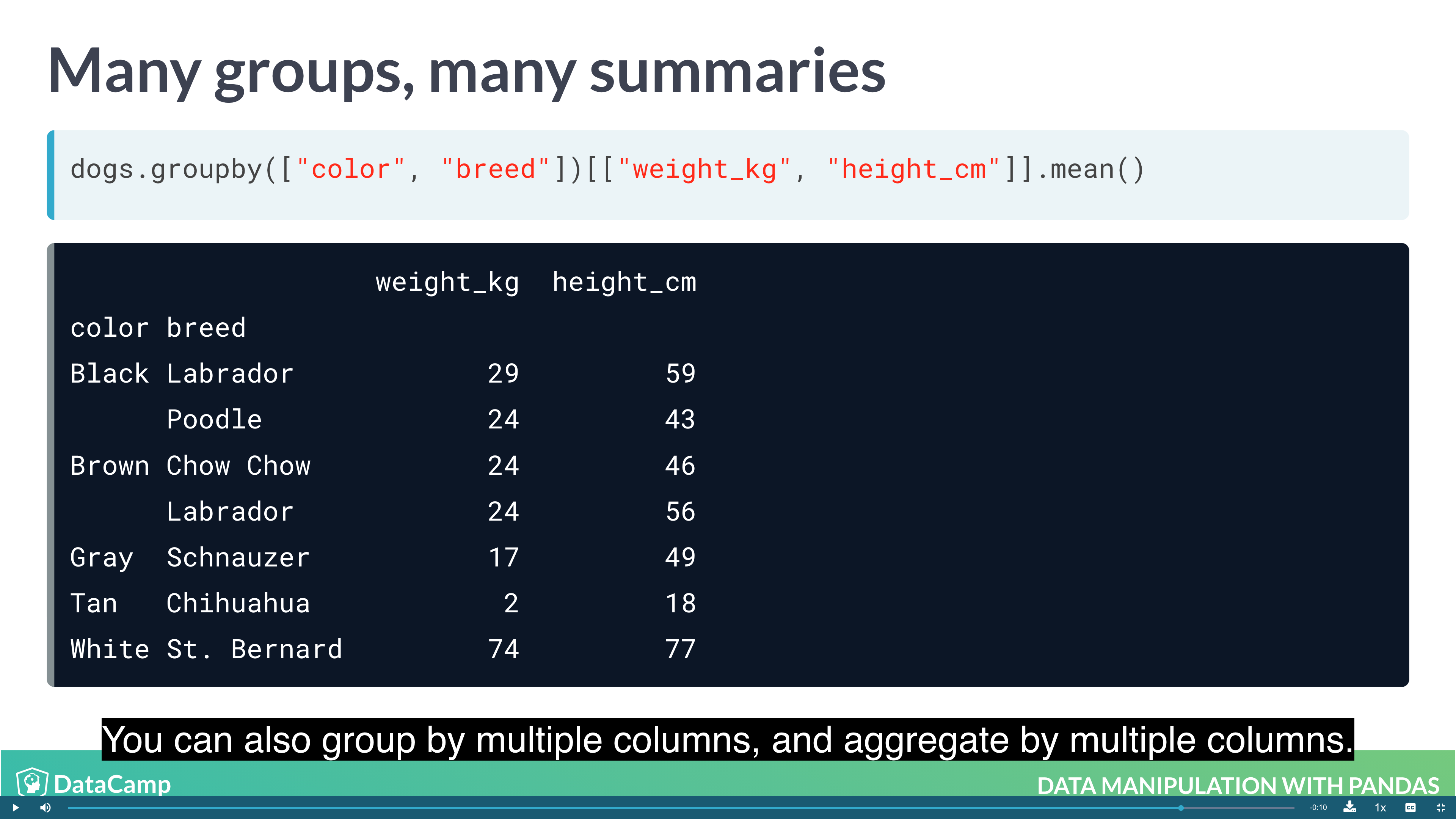
1 | dogs.groupby(["colors", "breed"])[["weight_ky", "height_cm"]].mean() |
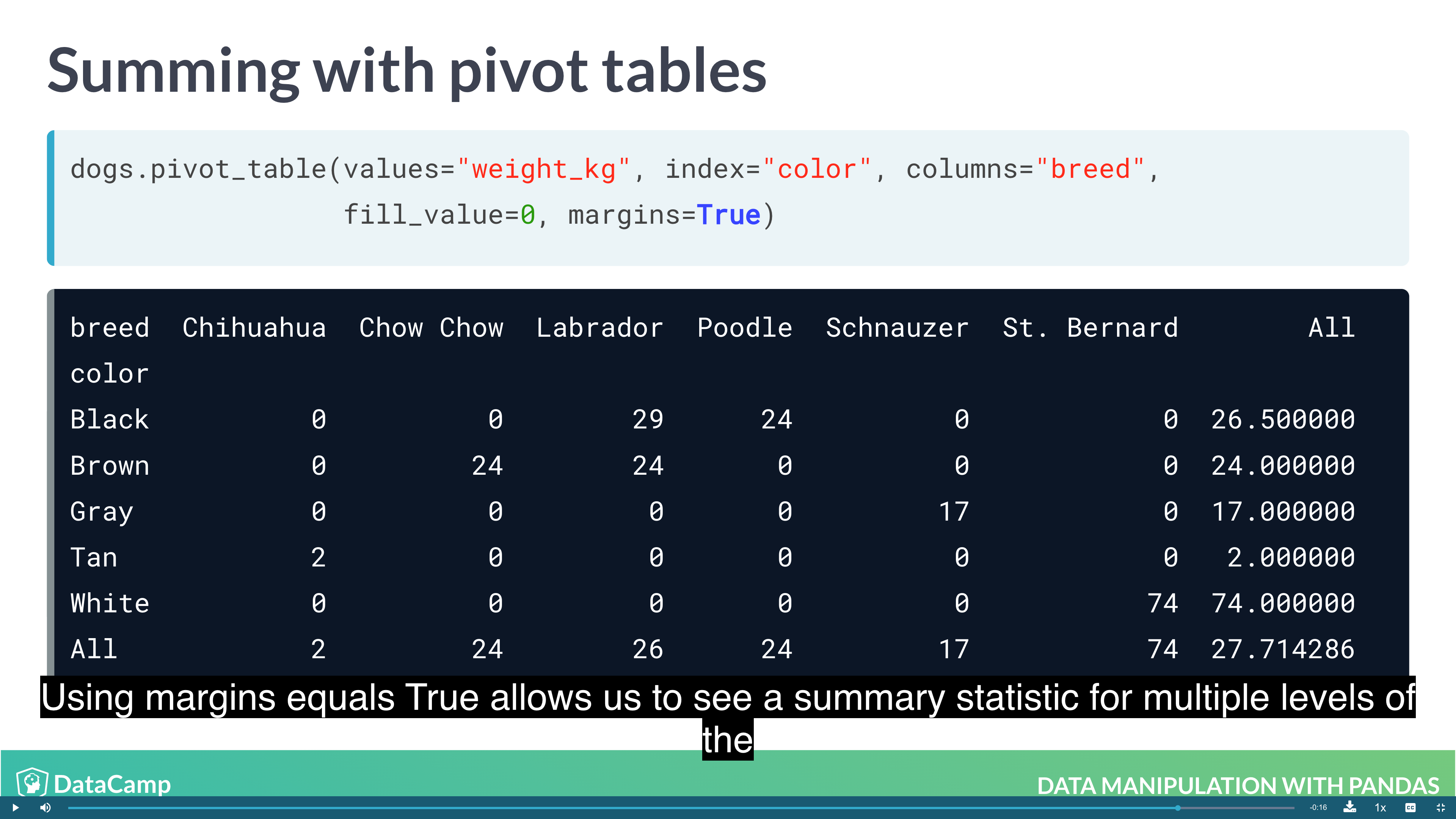
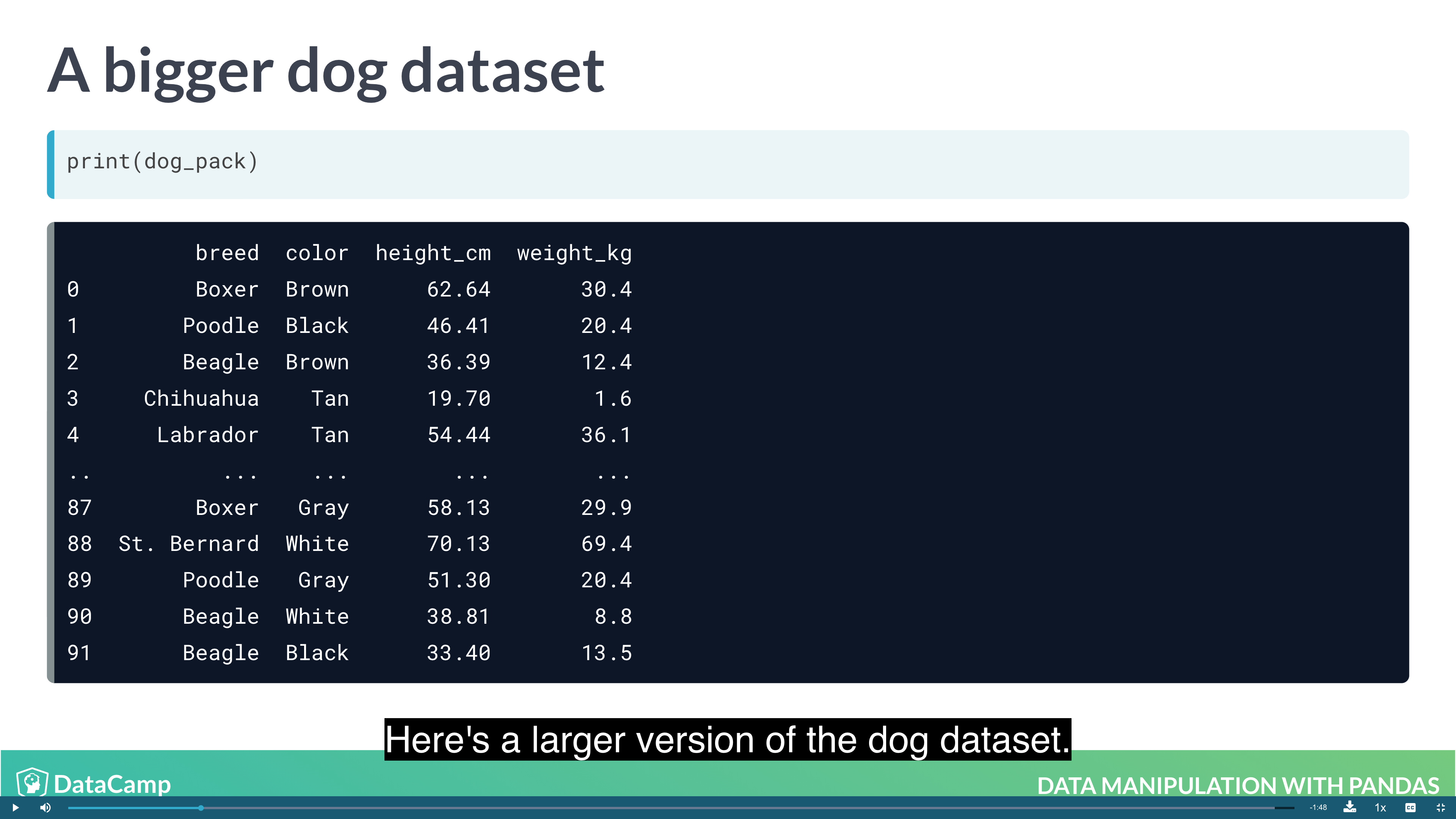
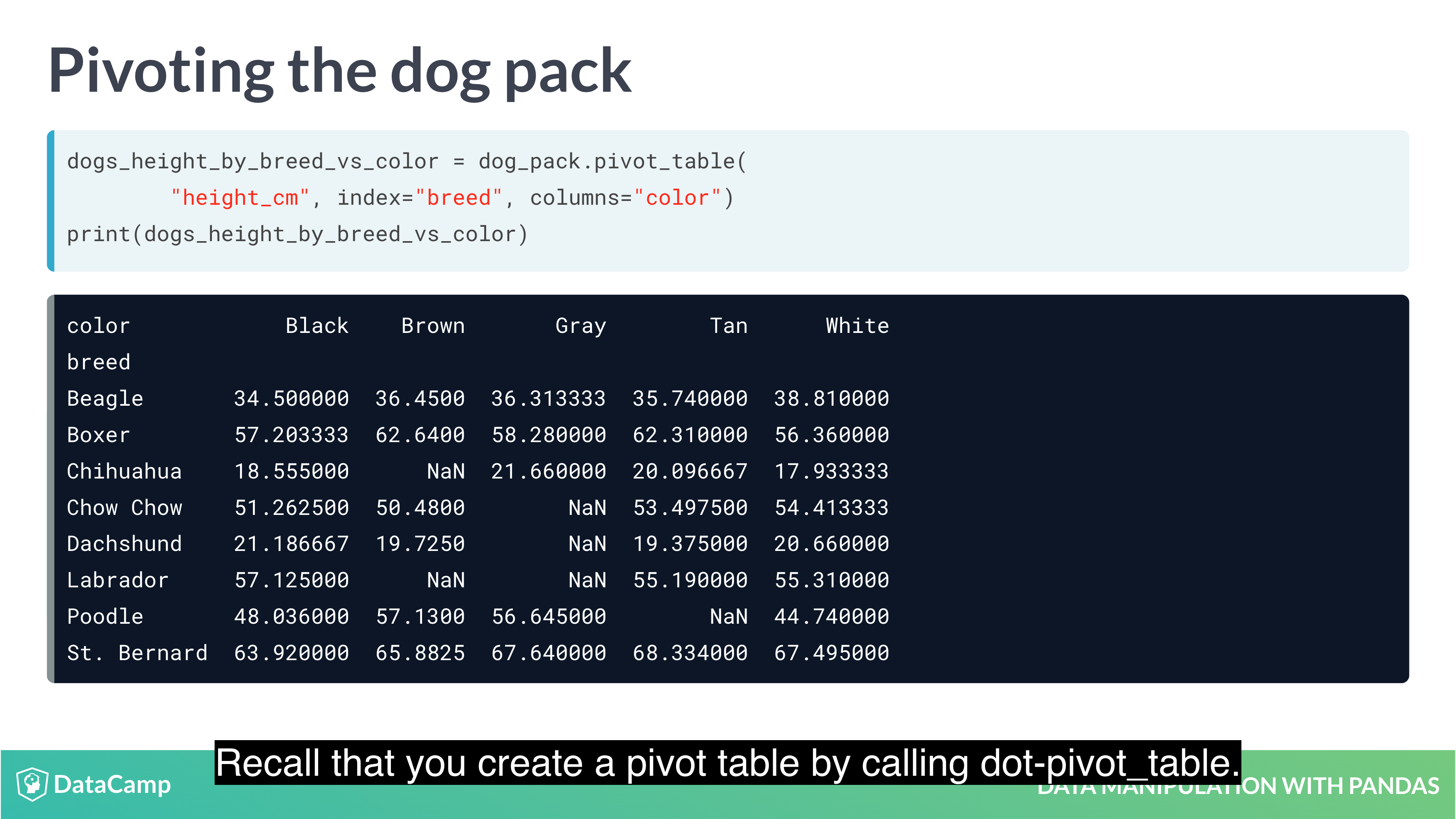
Pivot Tables
Pivot tables are the standard way of aggregating data in spreadsheets. In pandas, pivot tables are essentially just another way of performing grouped calculations. That is, the .pivot_table() method is just an alternative to .groupby().
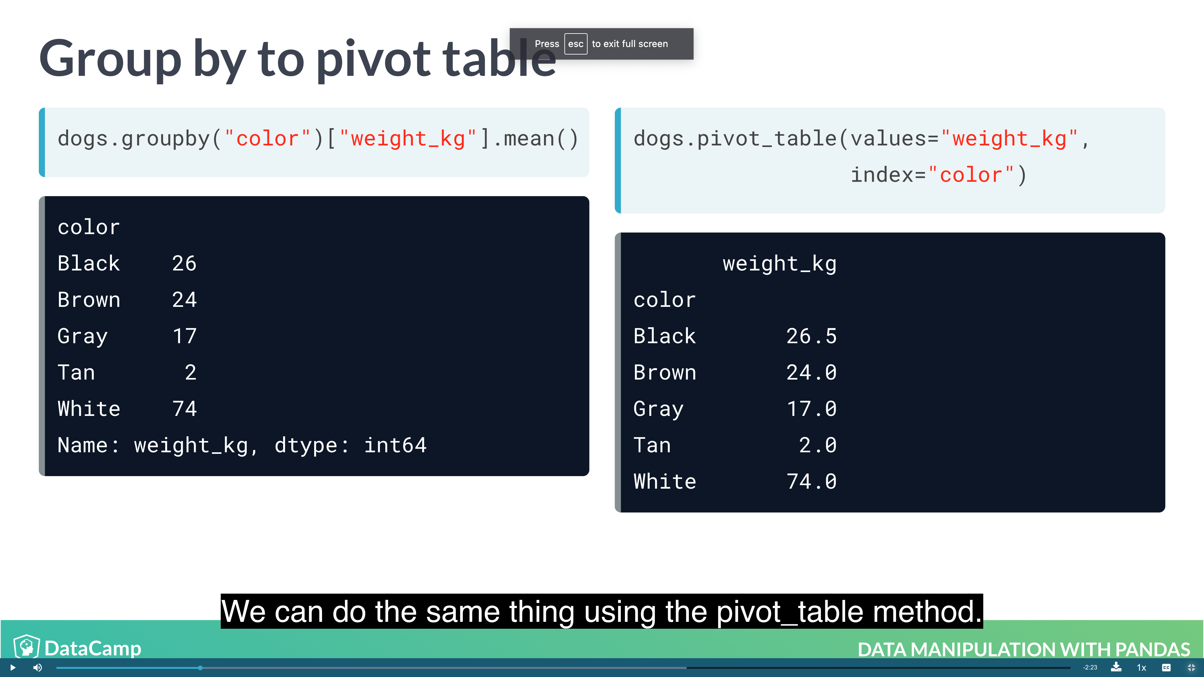
1 | dogs.groupby("color")["weight_kg"].mean() |
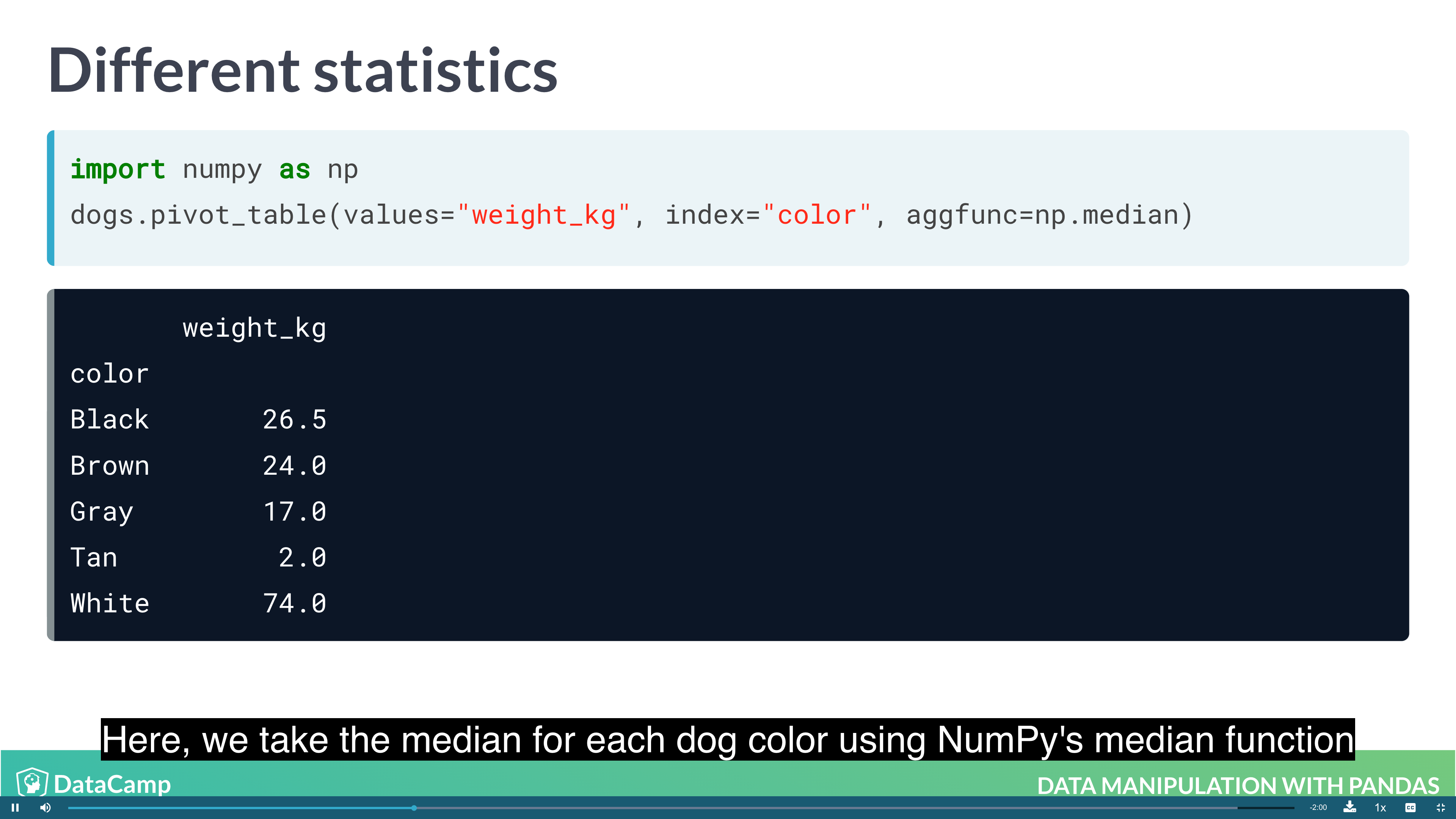
1 | # By default, pivot_table takes the mean value for each group. For other summary statistic, using numpy |
1 | # By default, pivot_table takes the mean value for each group. For other summary statistic, using numpy |
Slicing and Indexing Data
- Subsetting using slicing
- Indexes and subsetting using indexs
Explicit indexes
Pandas allows you to designate columns as an index. This enables cleaner code when taking subsets (as well as providing more efficient lookup under some circumstances).
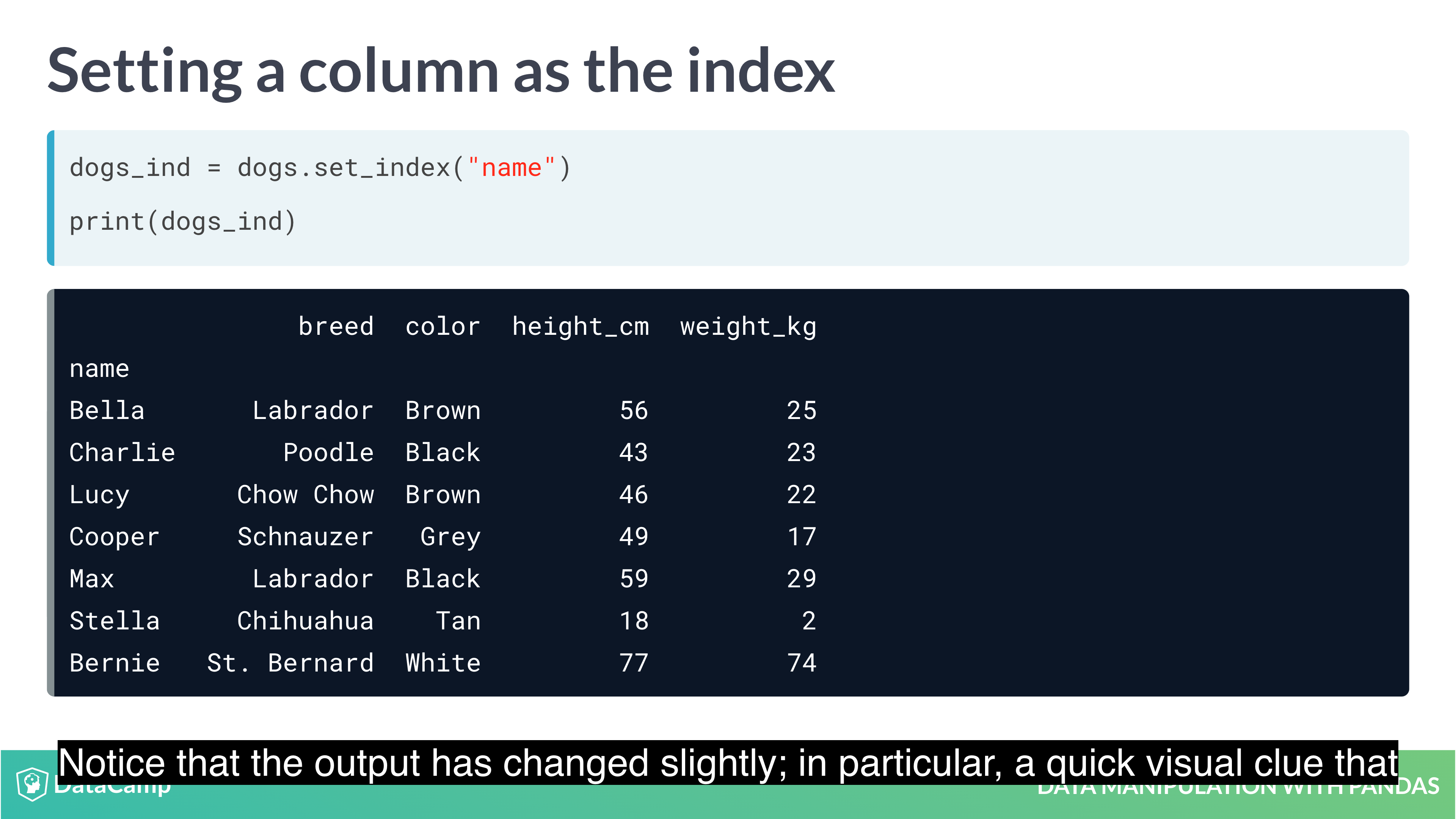
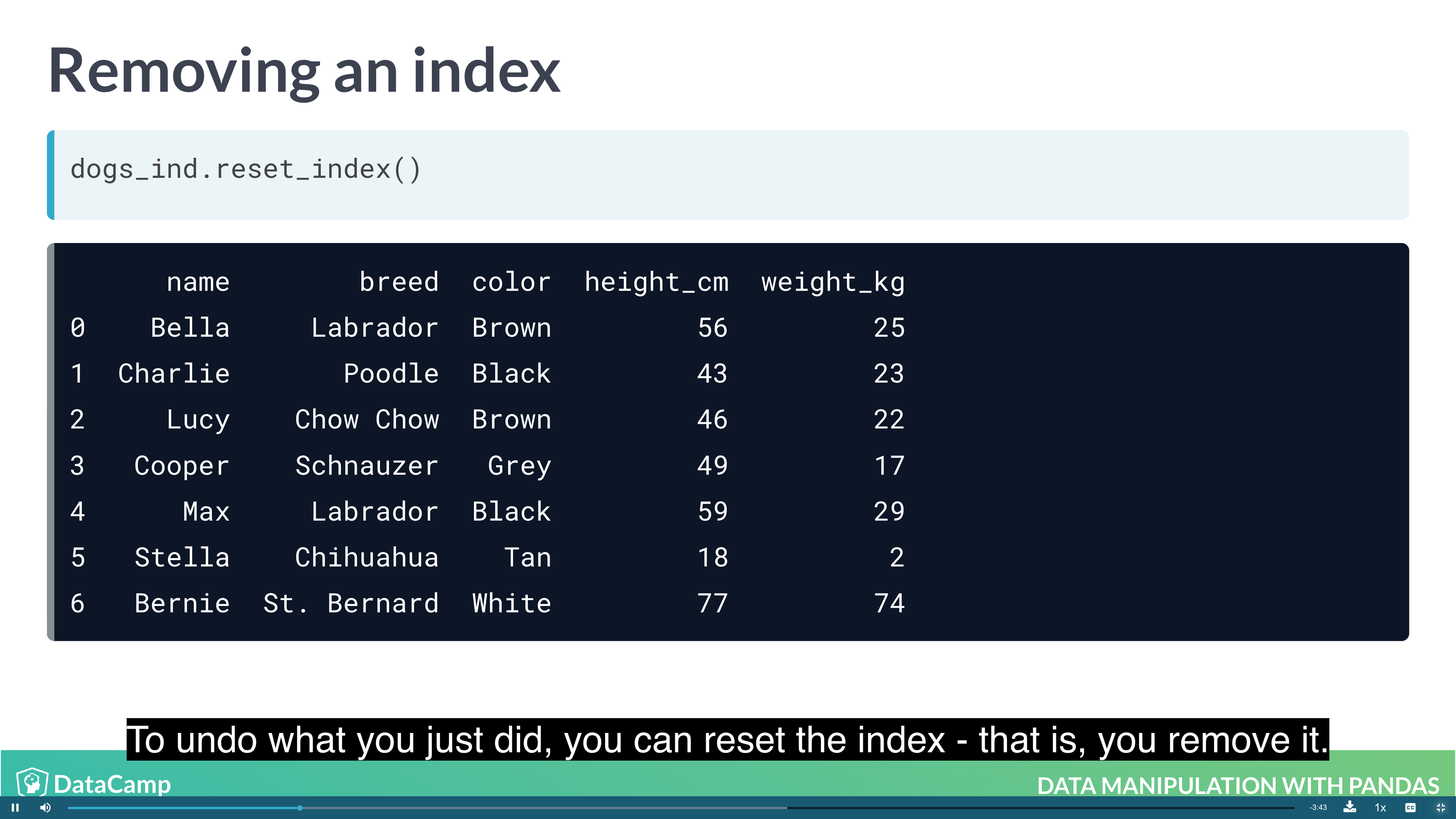
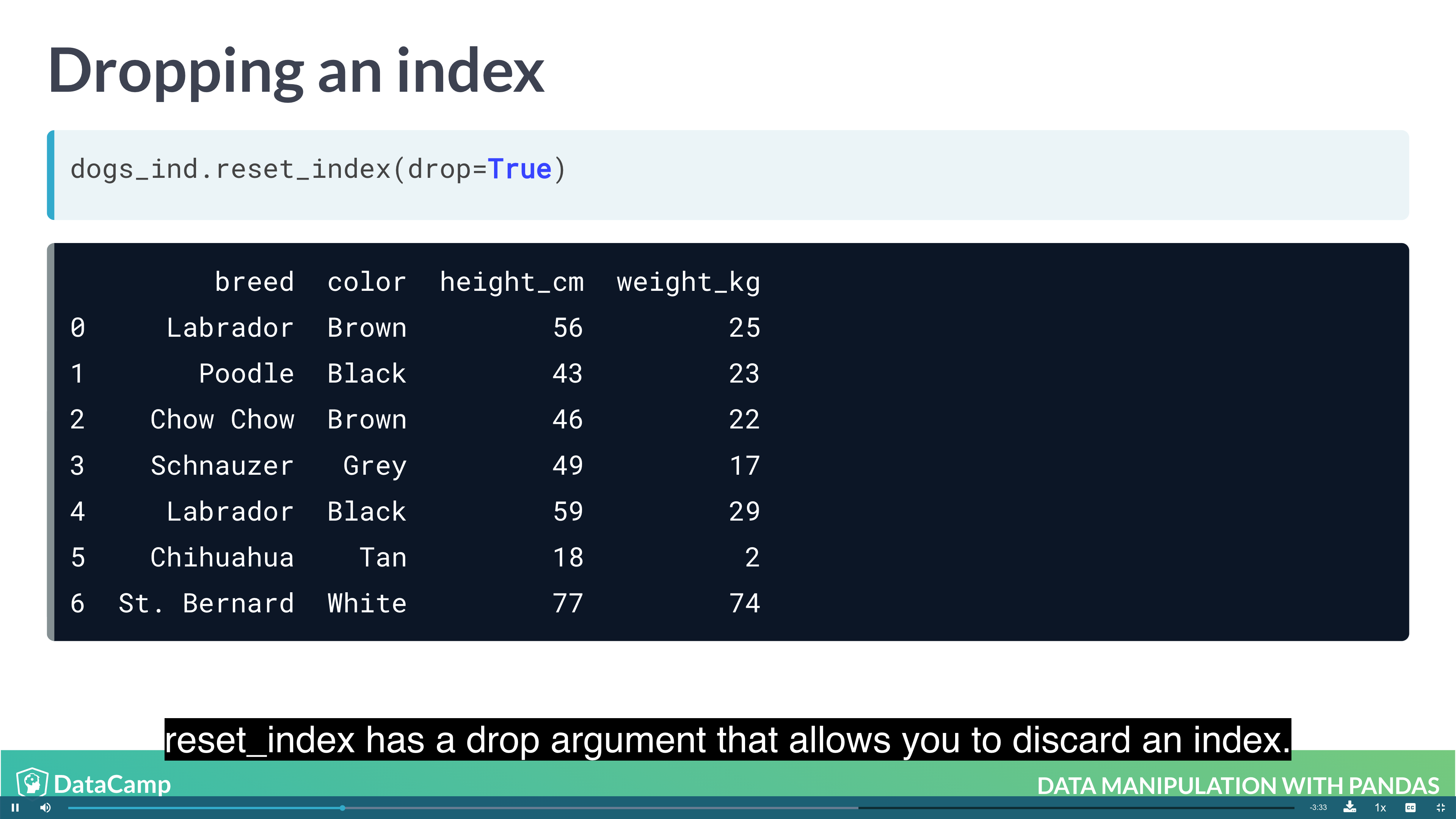
1 | df.set_index("name") # setting index; index doesn't have to be unique; index makes subsetting more readable |
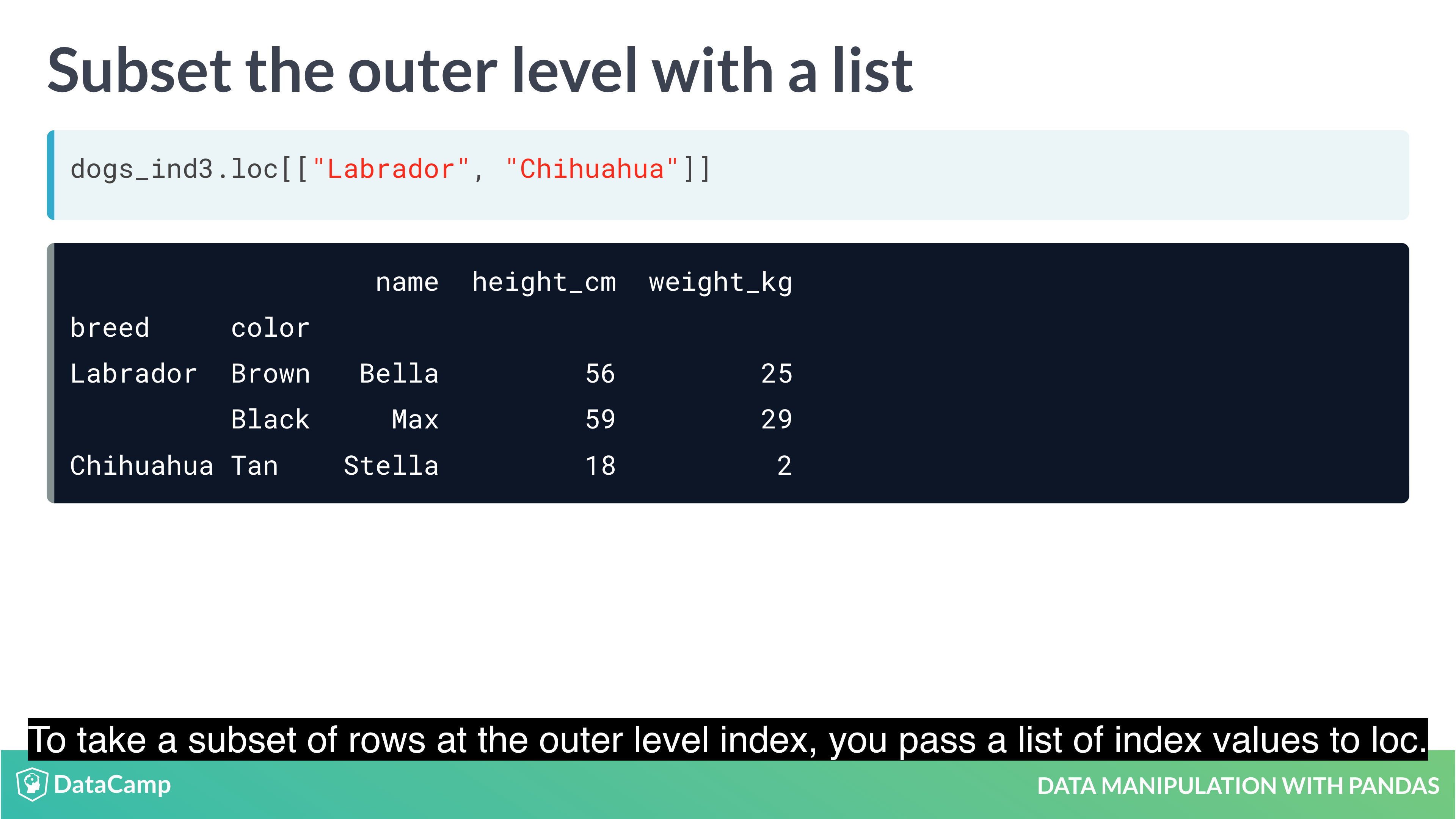
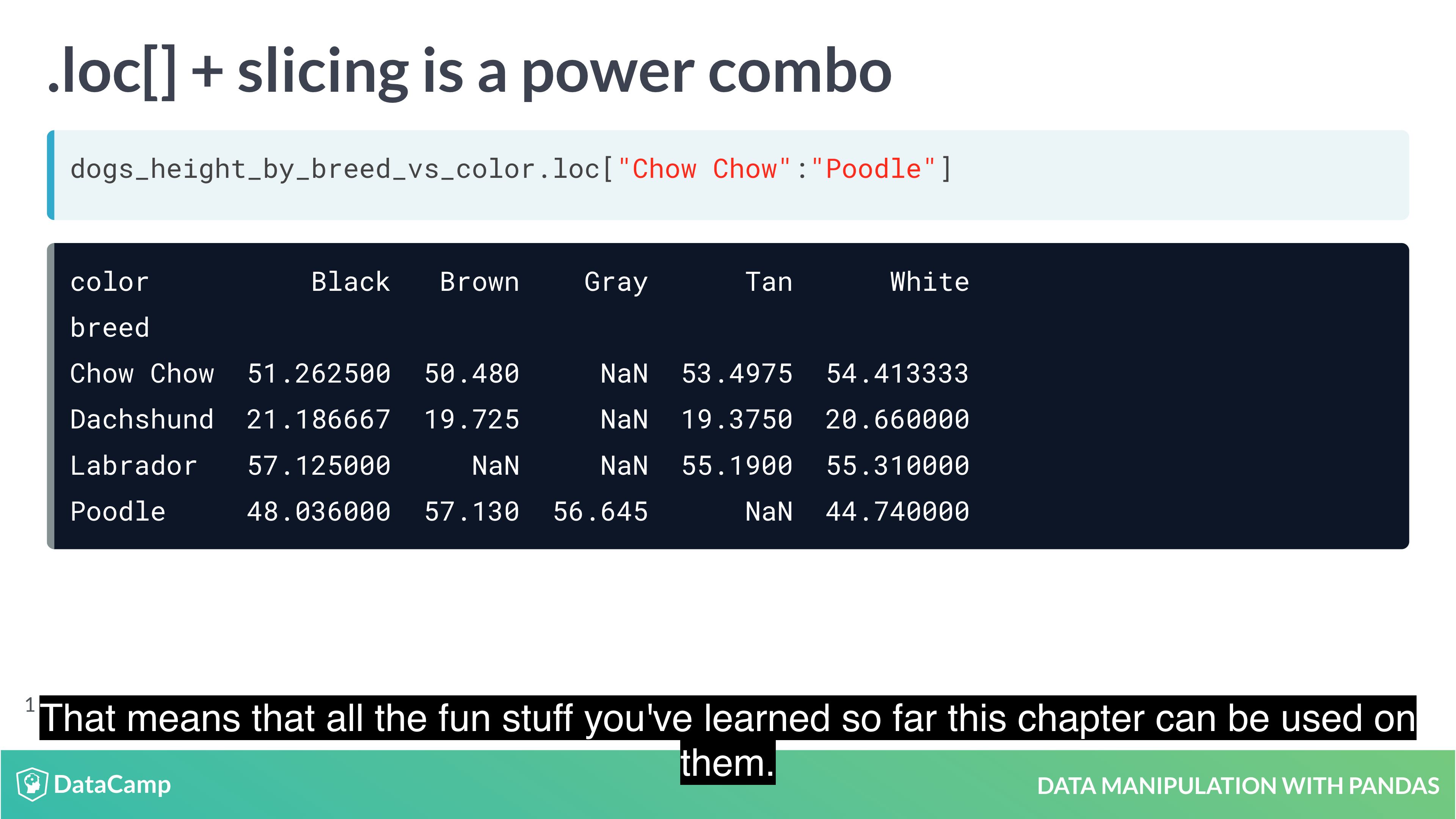
Subsetting with .loc[]
The killer feature for indexes is .loc[]: a subsetting method that accepts index values. When you pass it a single argument, it will take a subset of rows.
The code for subsetting using .loc[] can be easier to read than standard square bracket subsetting, which can make your code less burdensome to maintain.
1 | df[df["col"].isin(["val_1", "val_2"])] |
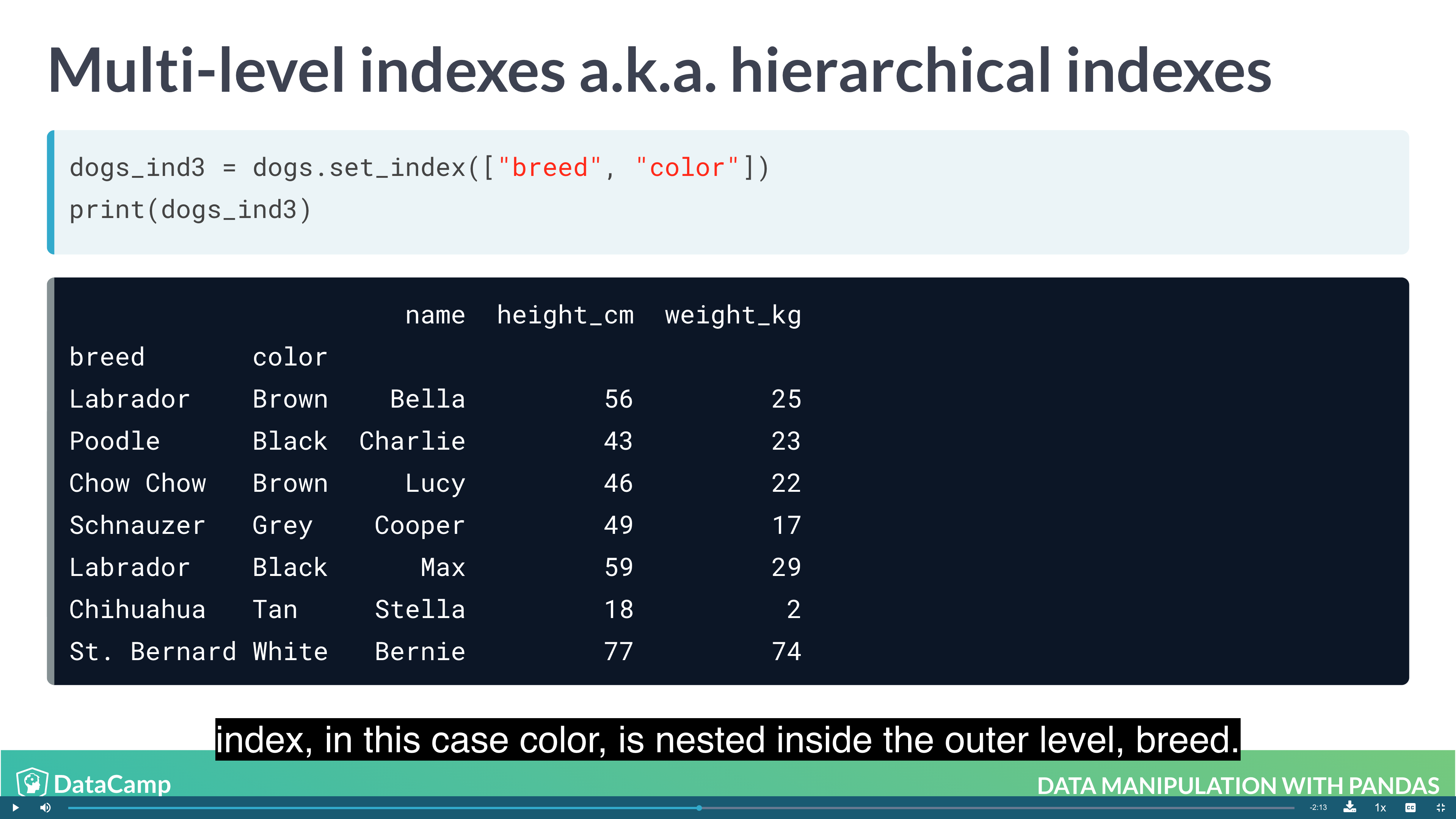
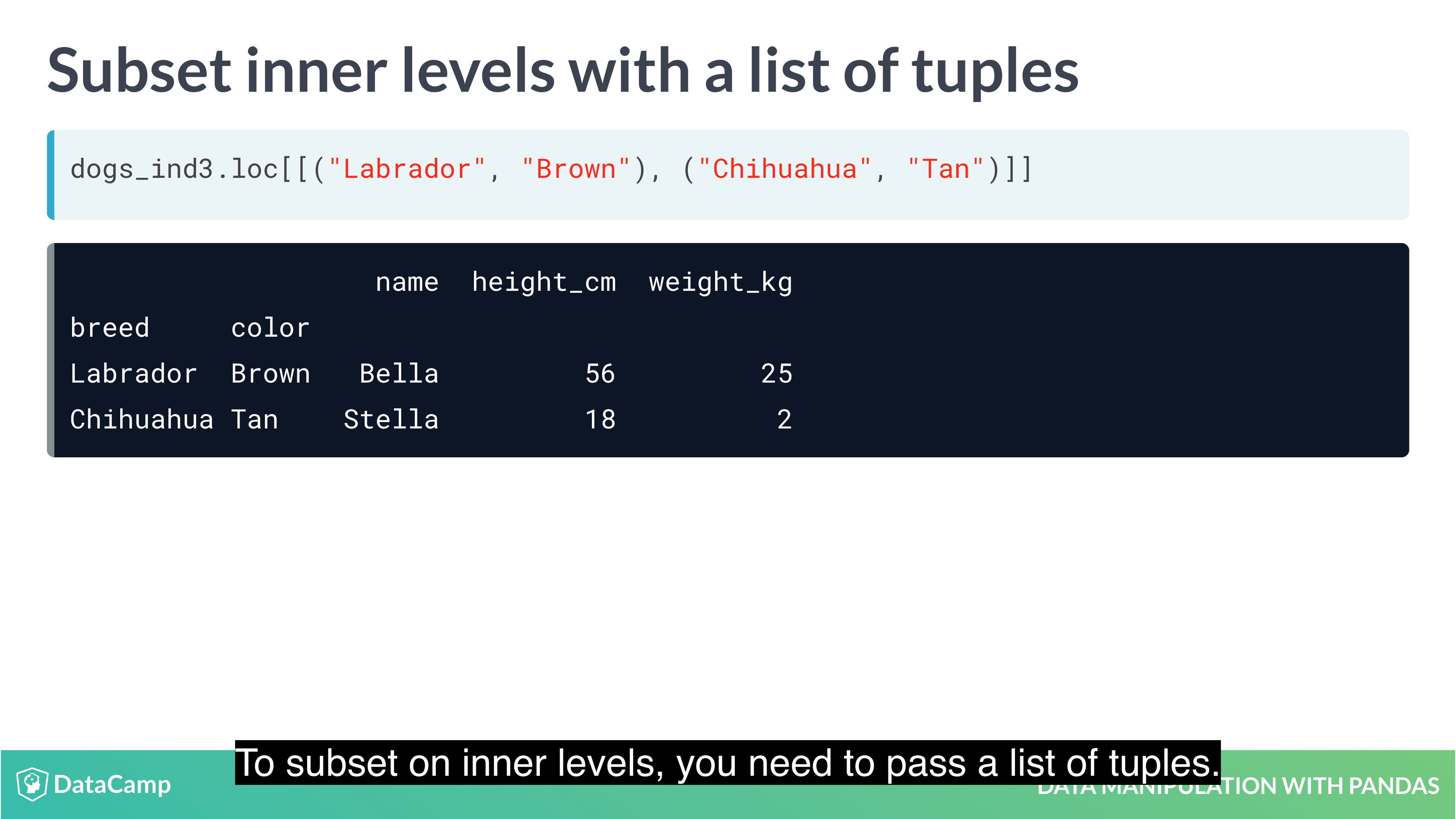
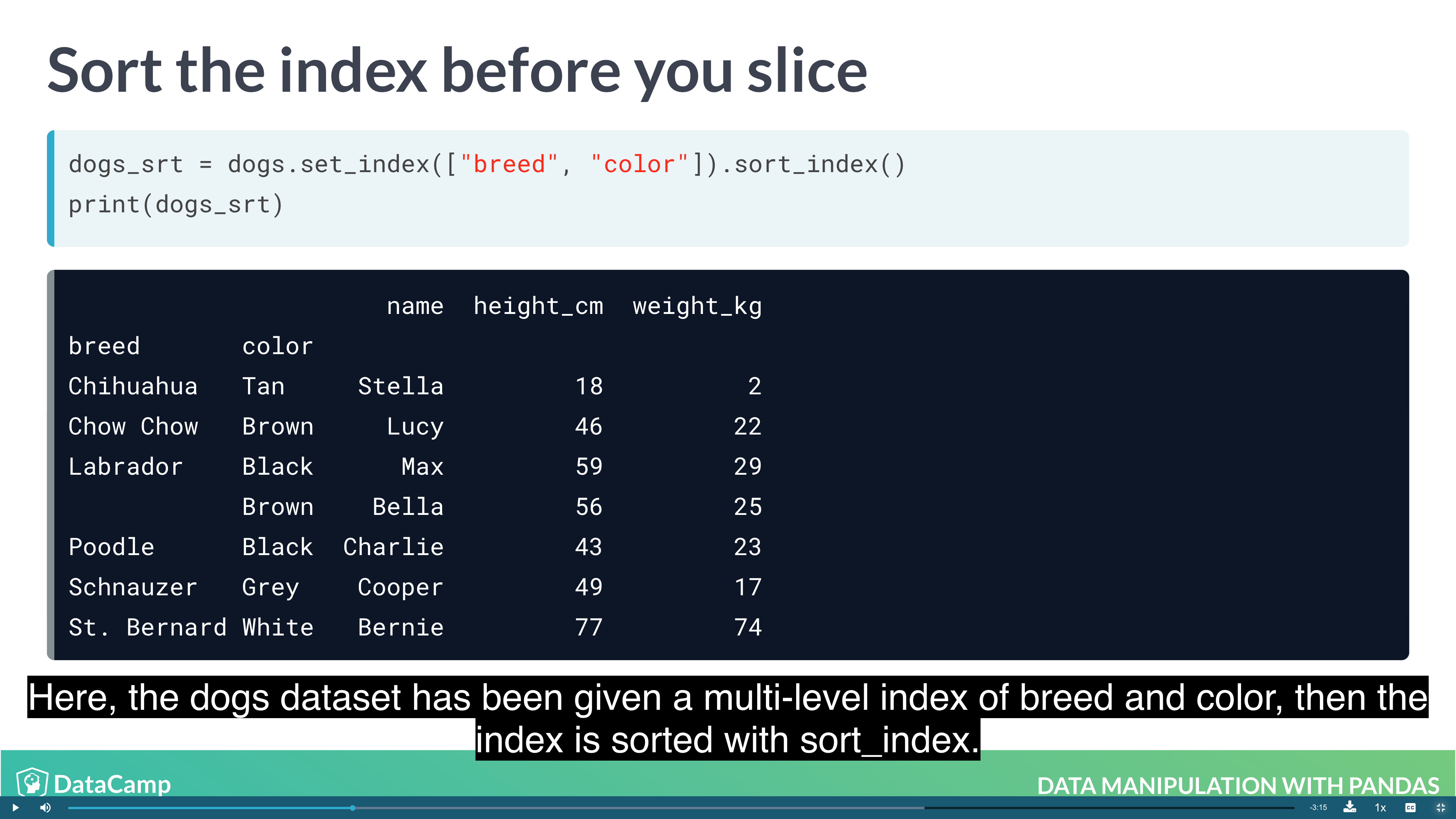
Setting multi-level indexes
Indexes can also be made out of multiple columns, forming a multi-level index (sometimes called a hierarchical index). There is a trade-off to using these.
The benefit is that multi-level indexes make it more natural to reason about nested categorical variables. For example, in a clinical trial you might have control and treatment groups. Then each test subject belongs to one or another group, and we can say that a test subject is nested inside treatment group. Similarly, in the temperature dataset, the city is located in the country, so we can say a city is nested inside country.
The main downside is that the code for manipulating indexes is different from the code for manipulating columns, so you have to learn two syntaxes, and keep track of how your data is represented.
1 | df_ind = df.set_index(["lev-1", "lev-2"]) # for example, lev-1 is country, lev-2 is state |
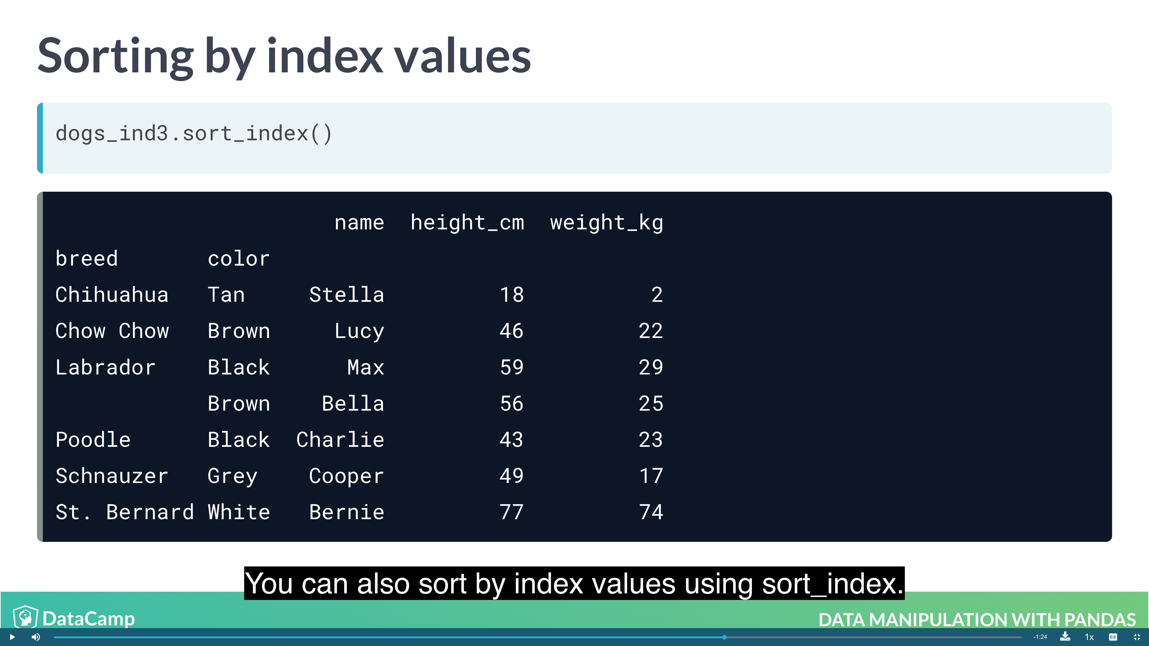
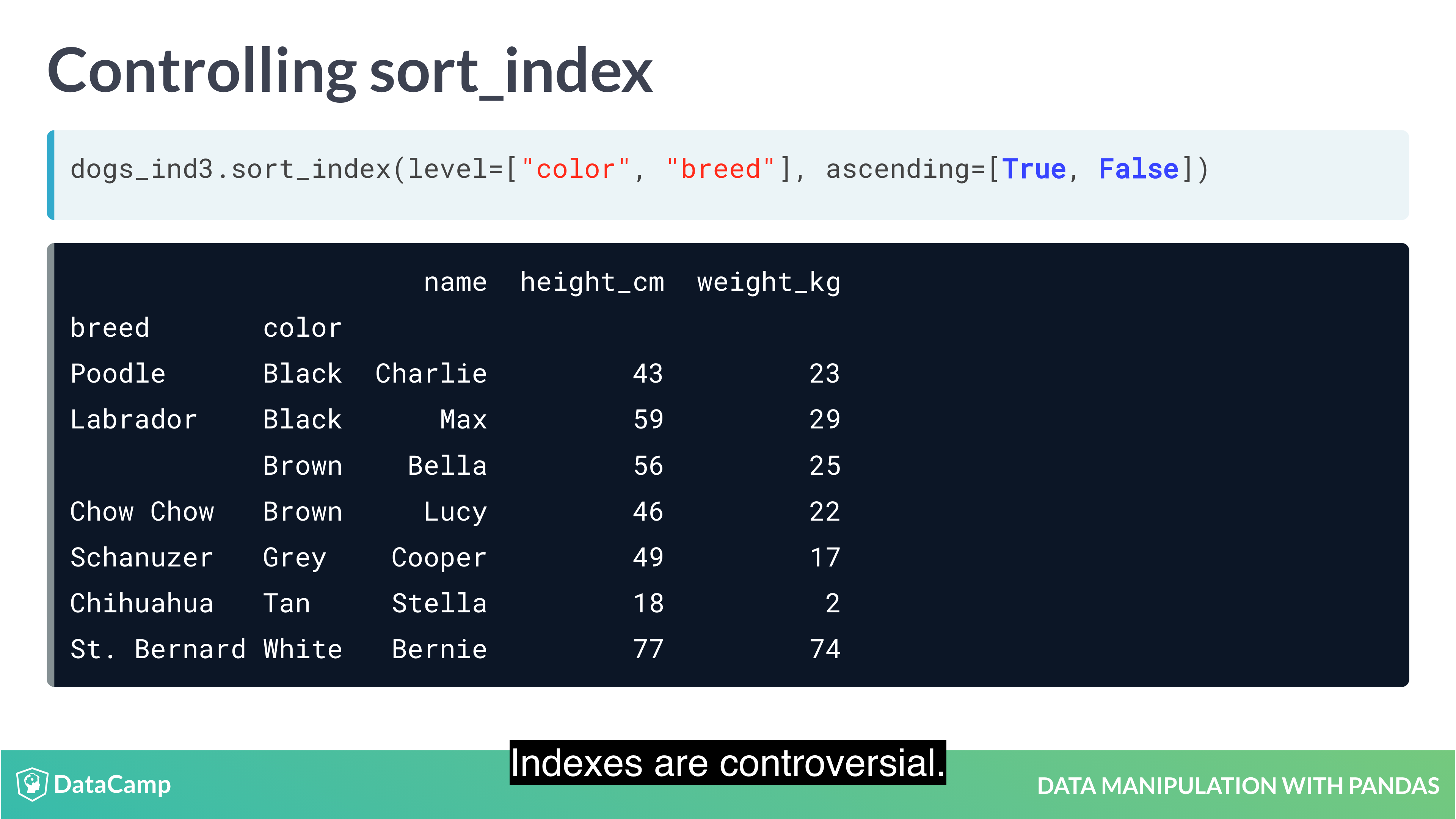
Sorting by index values
Previously, you changed the order of the rows in a DataFrame by calling .sort_values(). It’s also useful to be able to sort by elements in the index. For this, you need to use .sort_index().
1 | df.sort_index() |
Example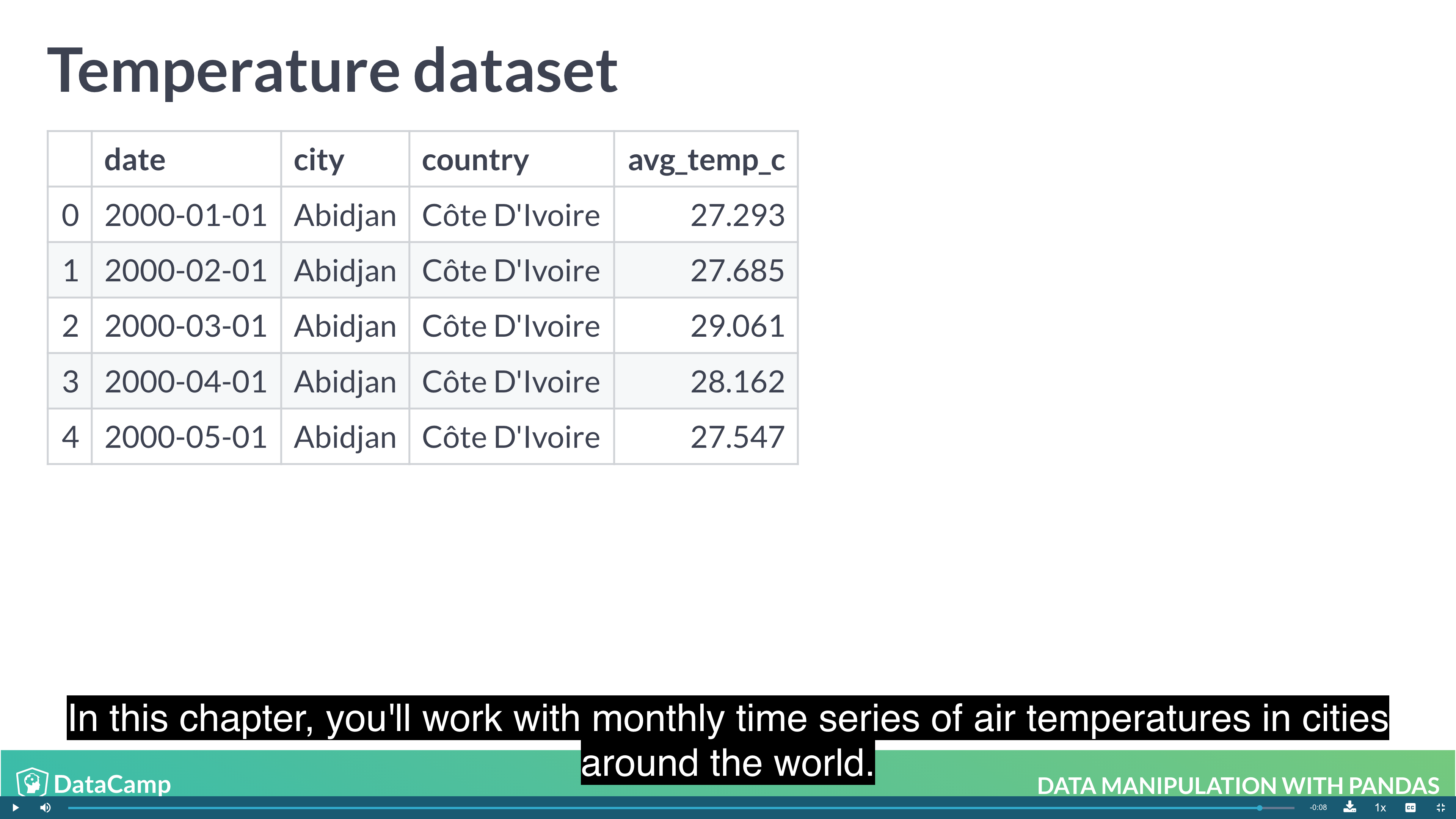
1 | # Look at temperatures |
Slicing and Subsetting with .loc and .iloc
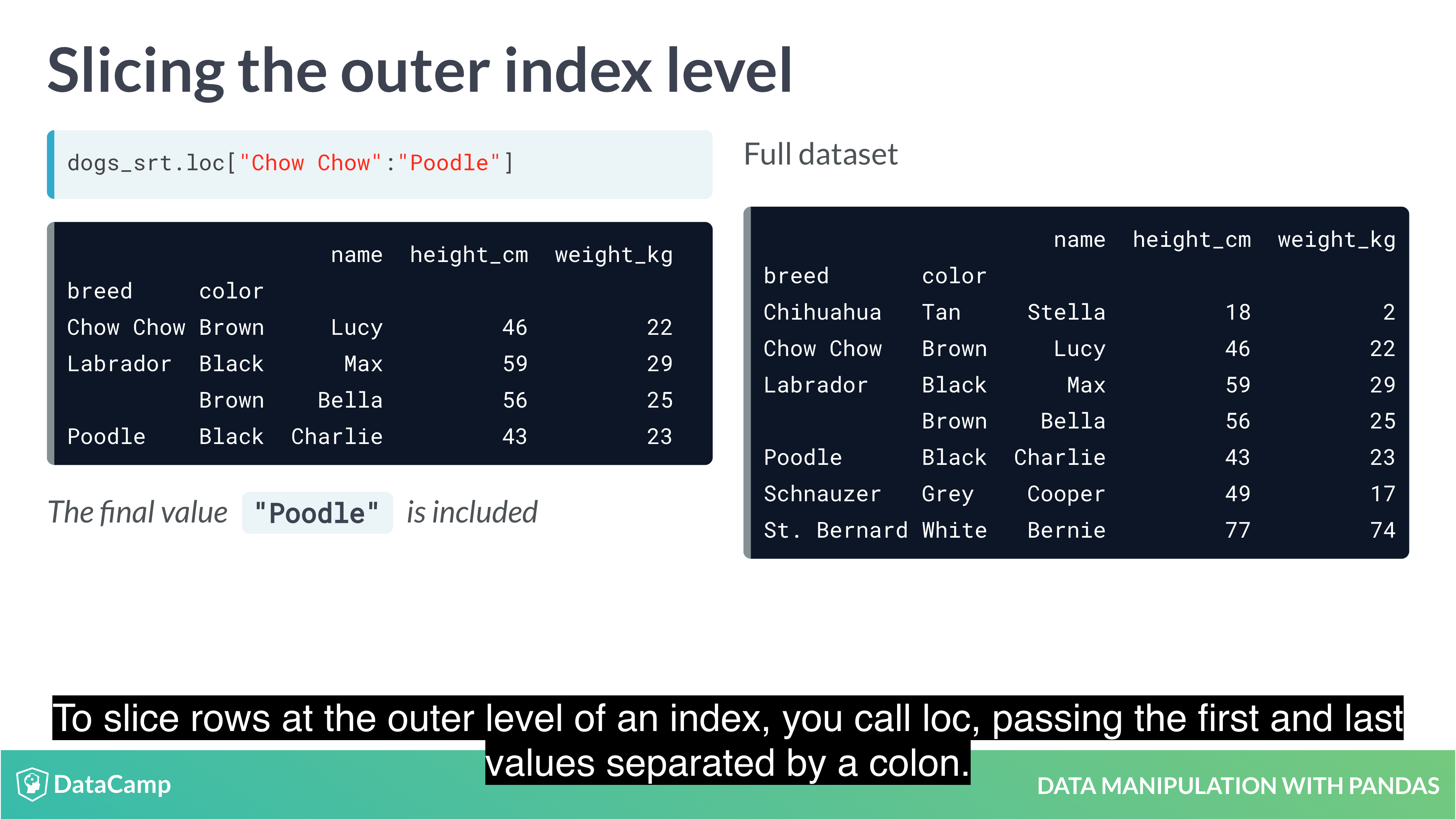
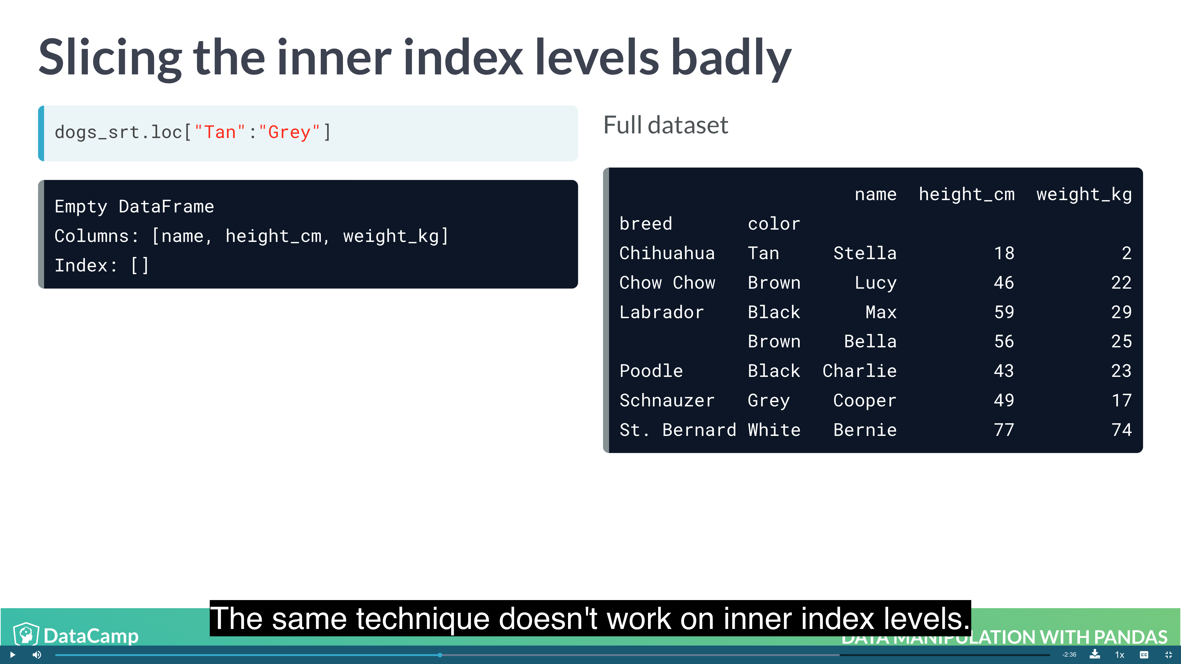
1 | # 1. Set indexes |
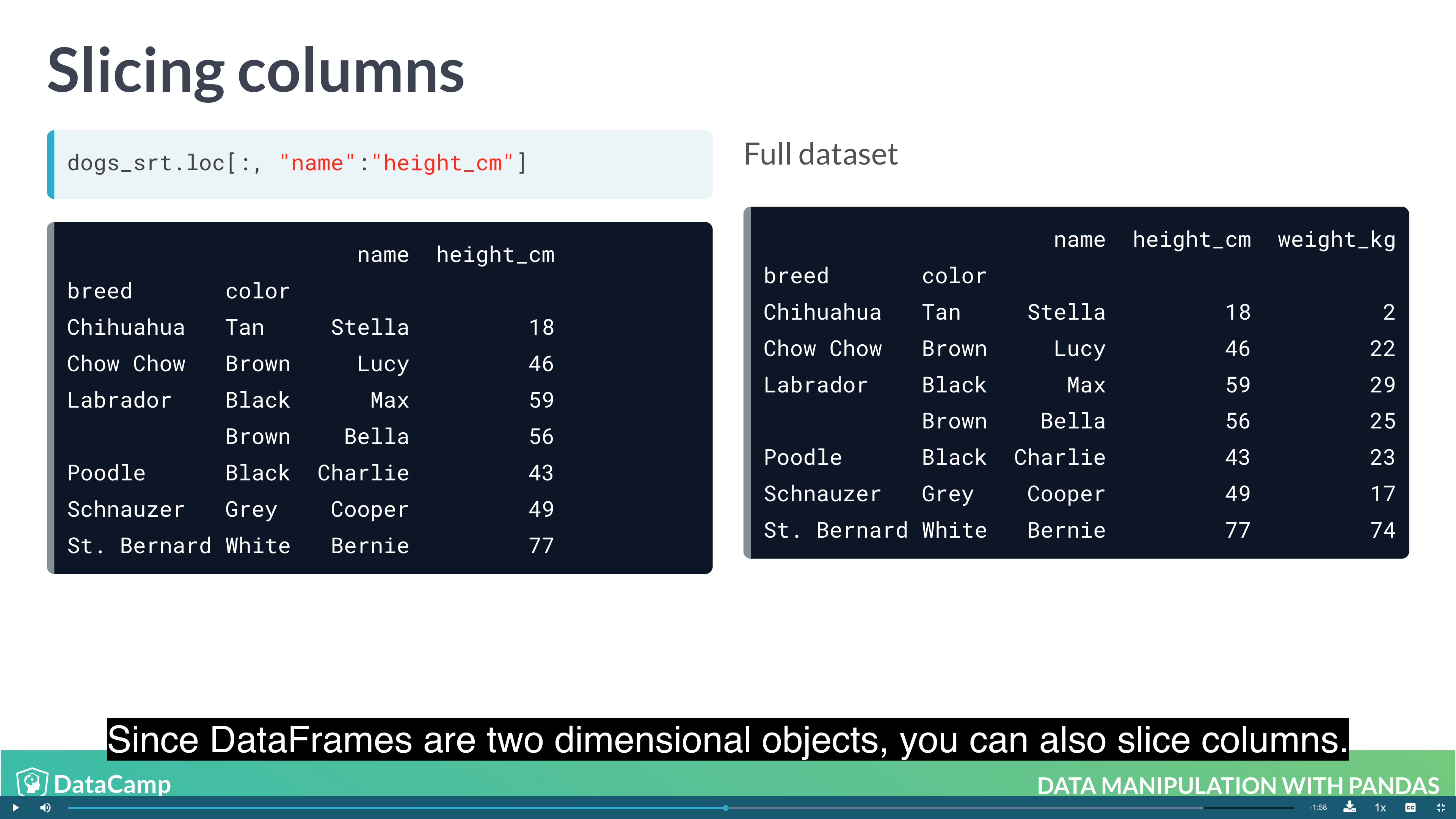
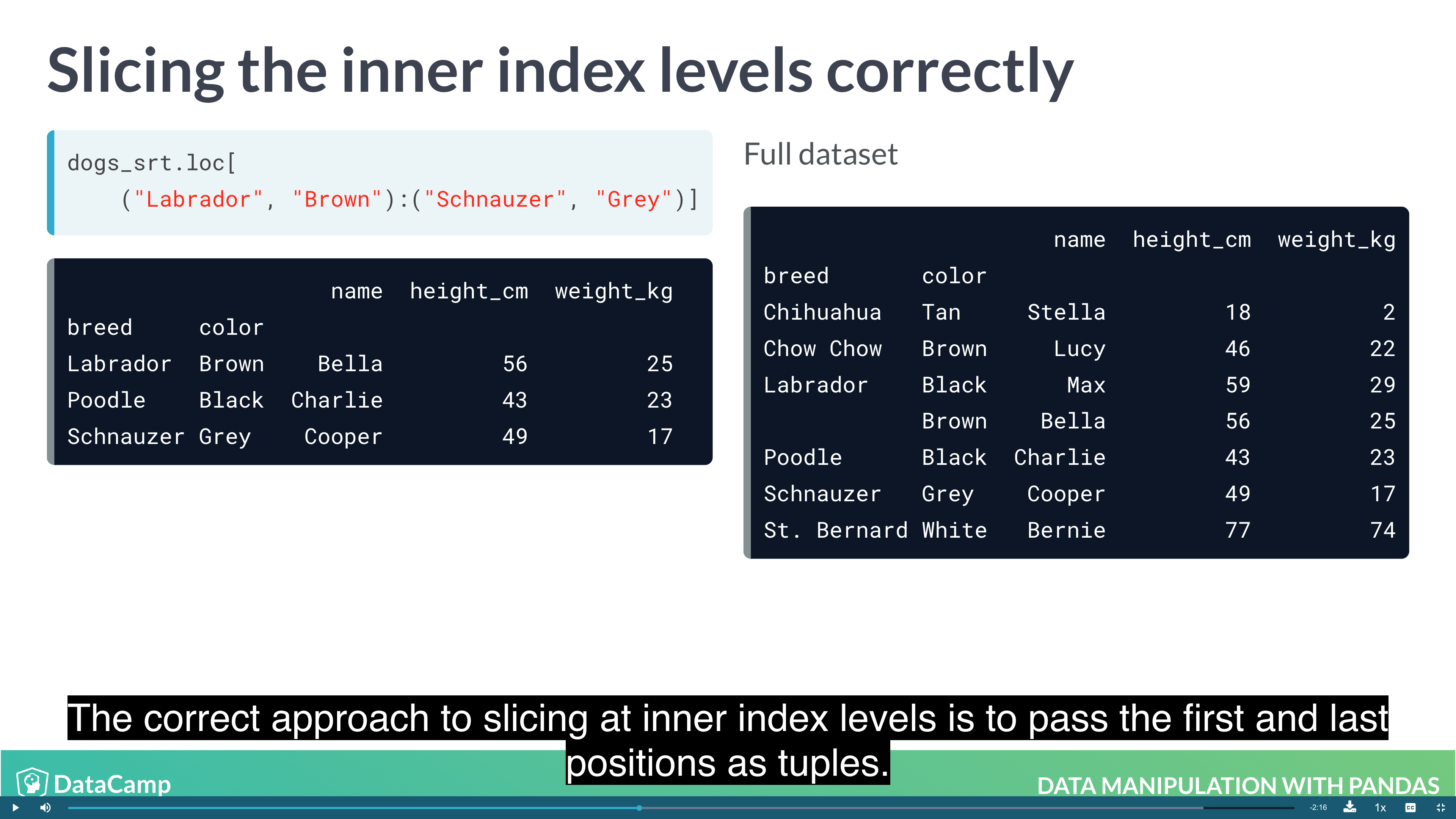
1 | df.loc["row_1":"row_2", "col_1":"col_2"] |
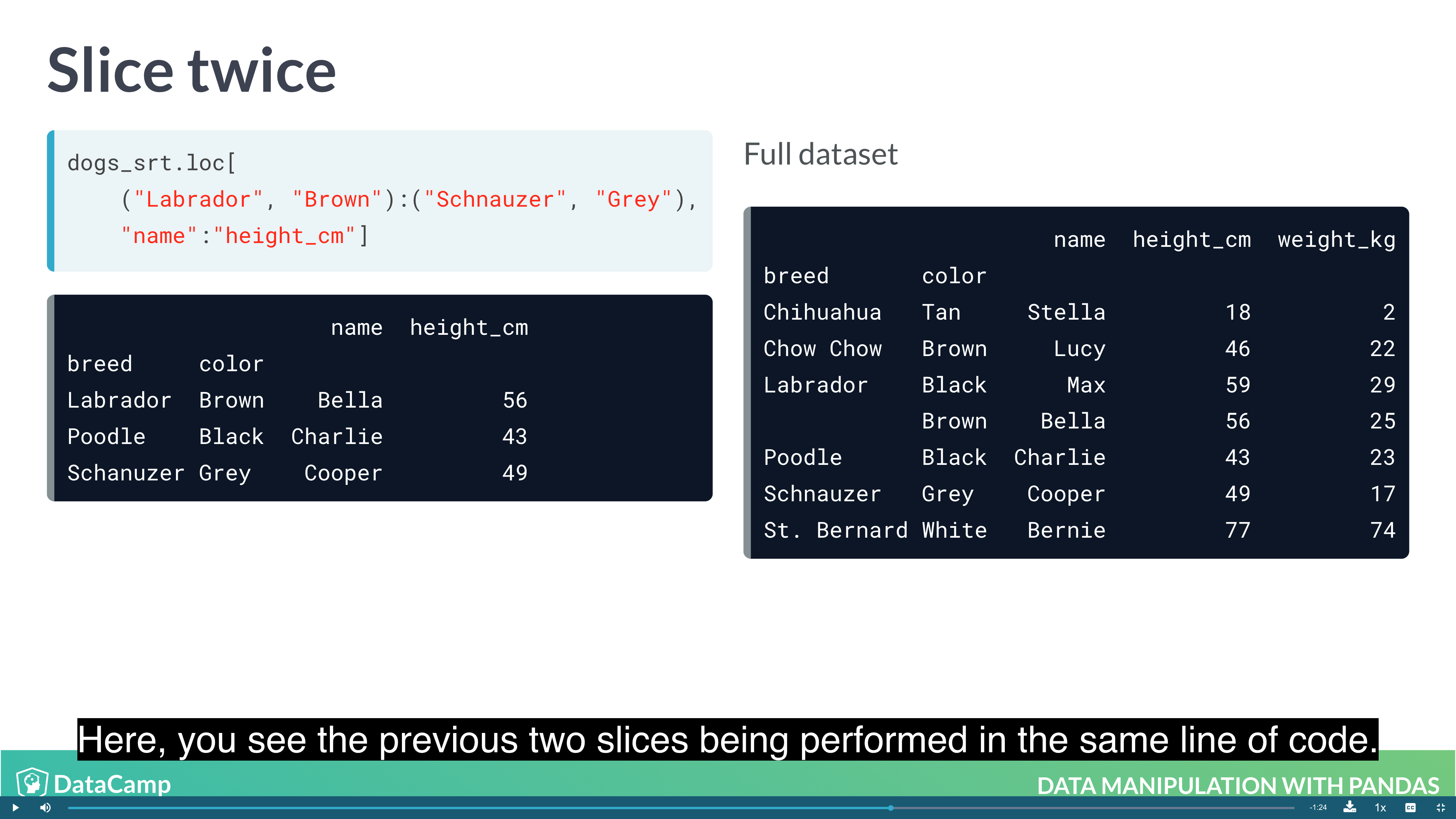
1 | df.loc[("outer_index_1", "inner_index_1"):("outer_index_2":"inner_index_2"), "col_1":"col_2"] |
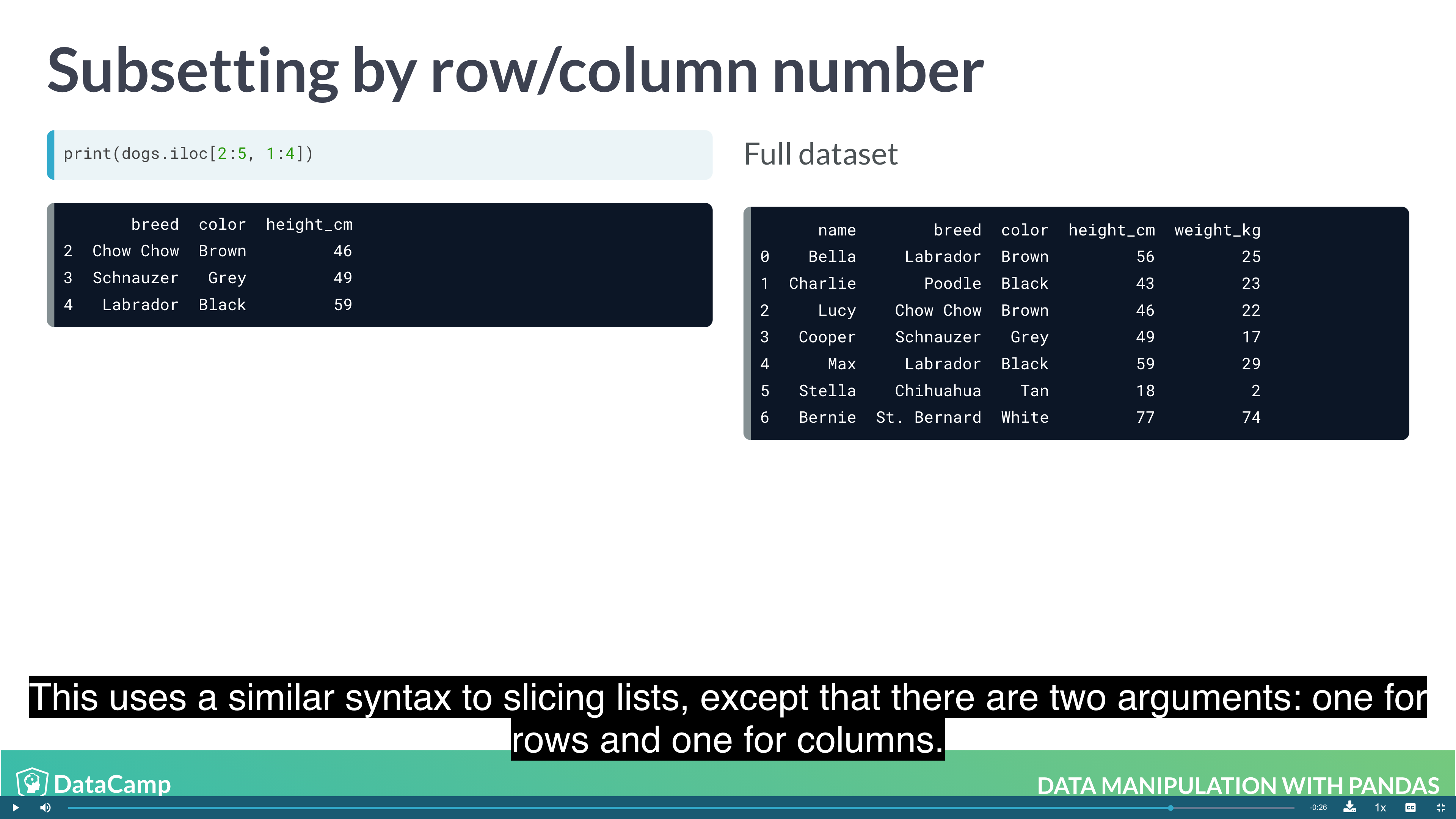
1 | df.iloc[n:m, n:m] |
Working with Pivot Tables
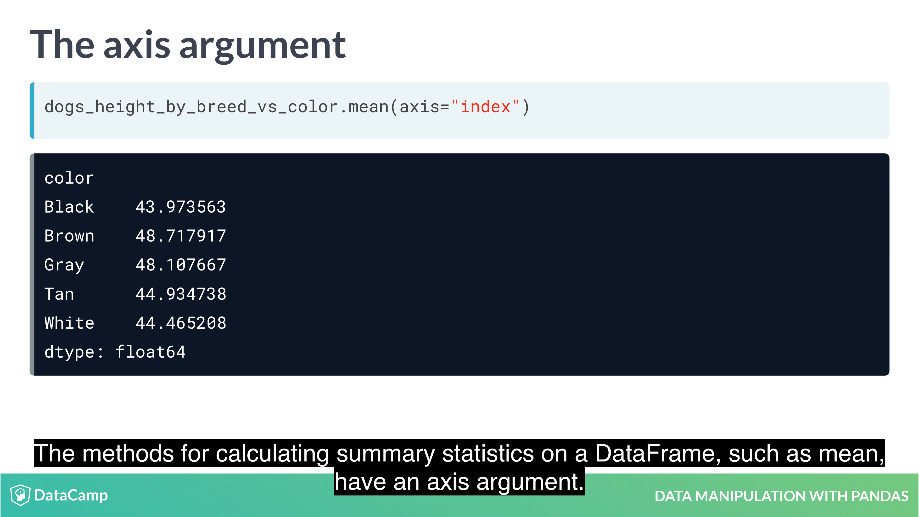
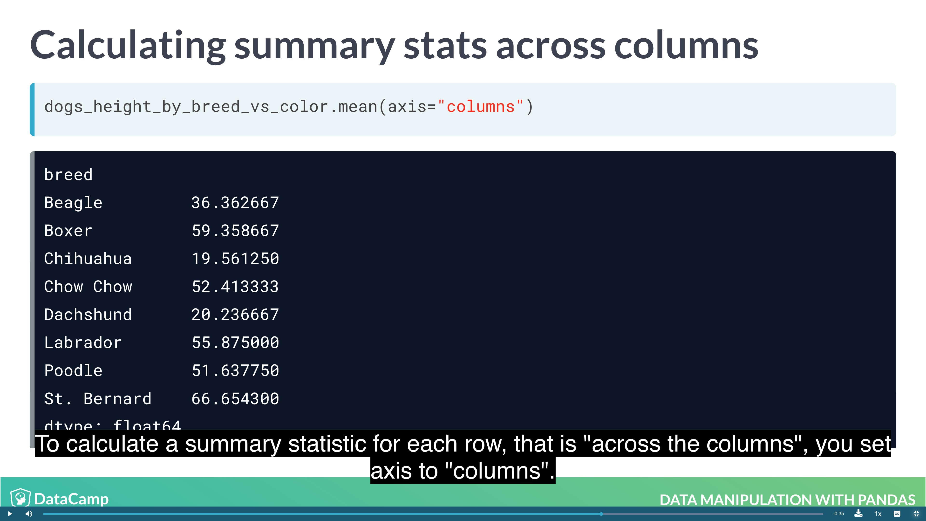
1 | df.mean(axis="index") # The default value is "index", which means "calculate the statistic across rows. |
You can access the components of a date (year, month and day) using code of the form dataframe["column"].dt.component. For example, the month component is dataframe["column"].dt.month, and the year component is dataframe["column"].dt.year.
Example
1 | # Add a year column to temperatures |
Creating and Visualizing Data
- Plotting
- Handling missing data
- Reading data into a DataFrame
Visualization
1 | import matplotlib.pyplot as plt |
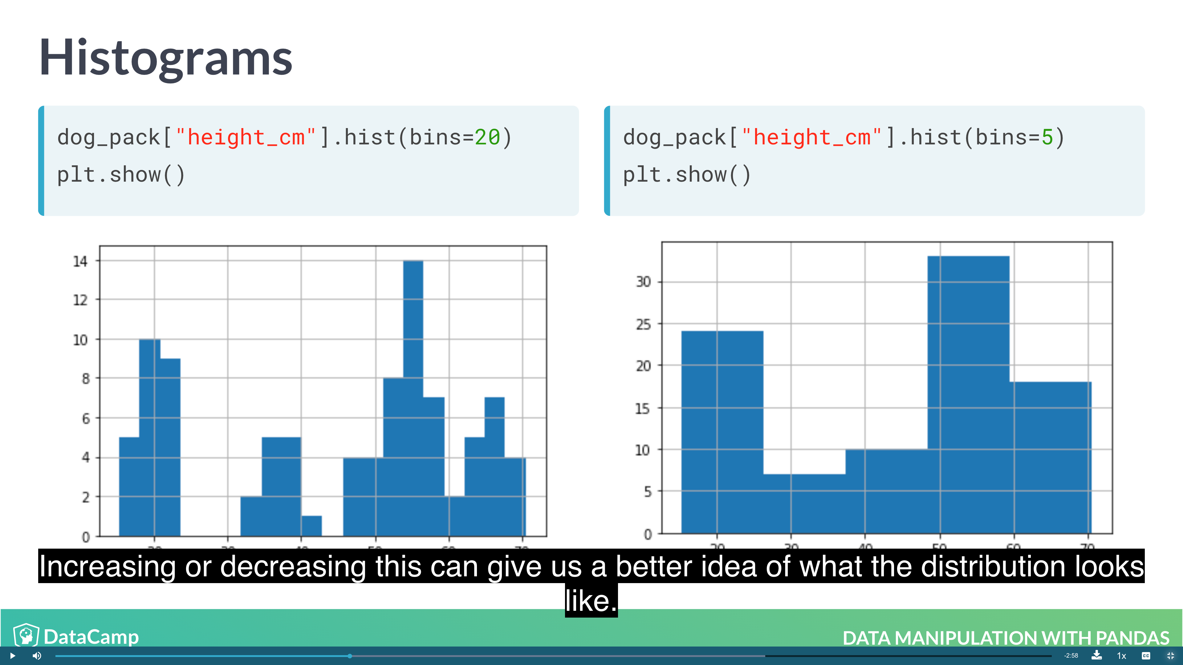
1 | # Histogram |
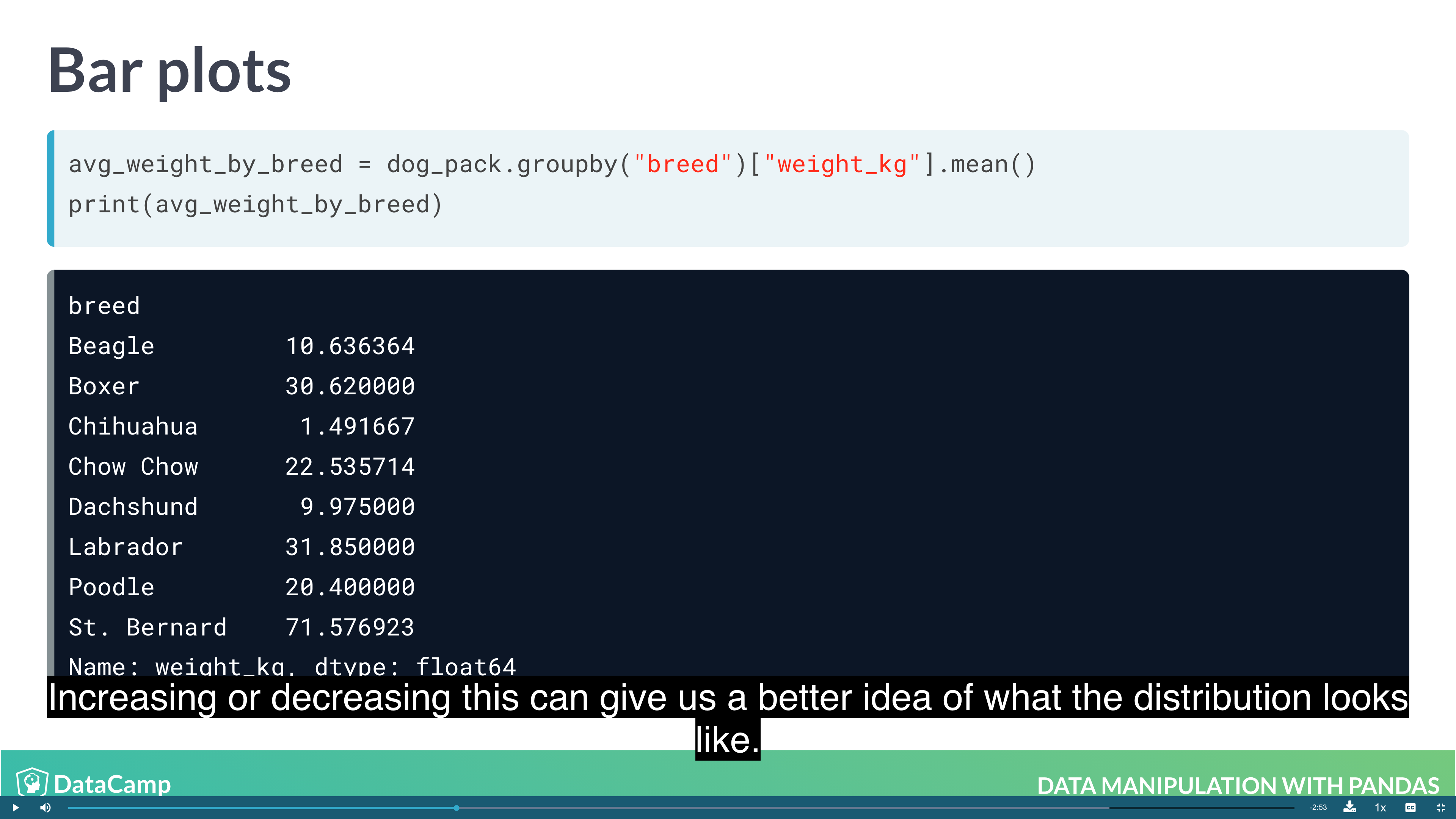
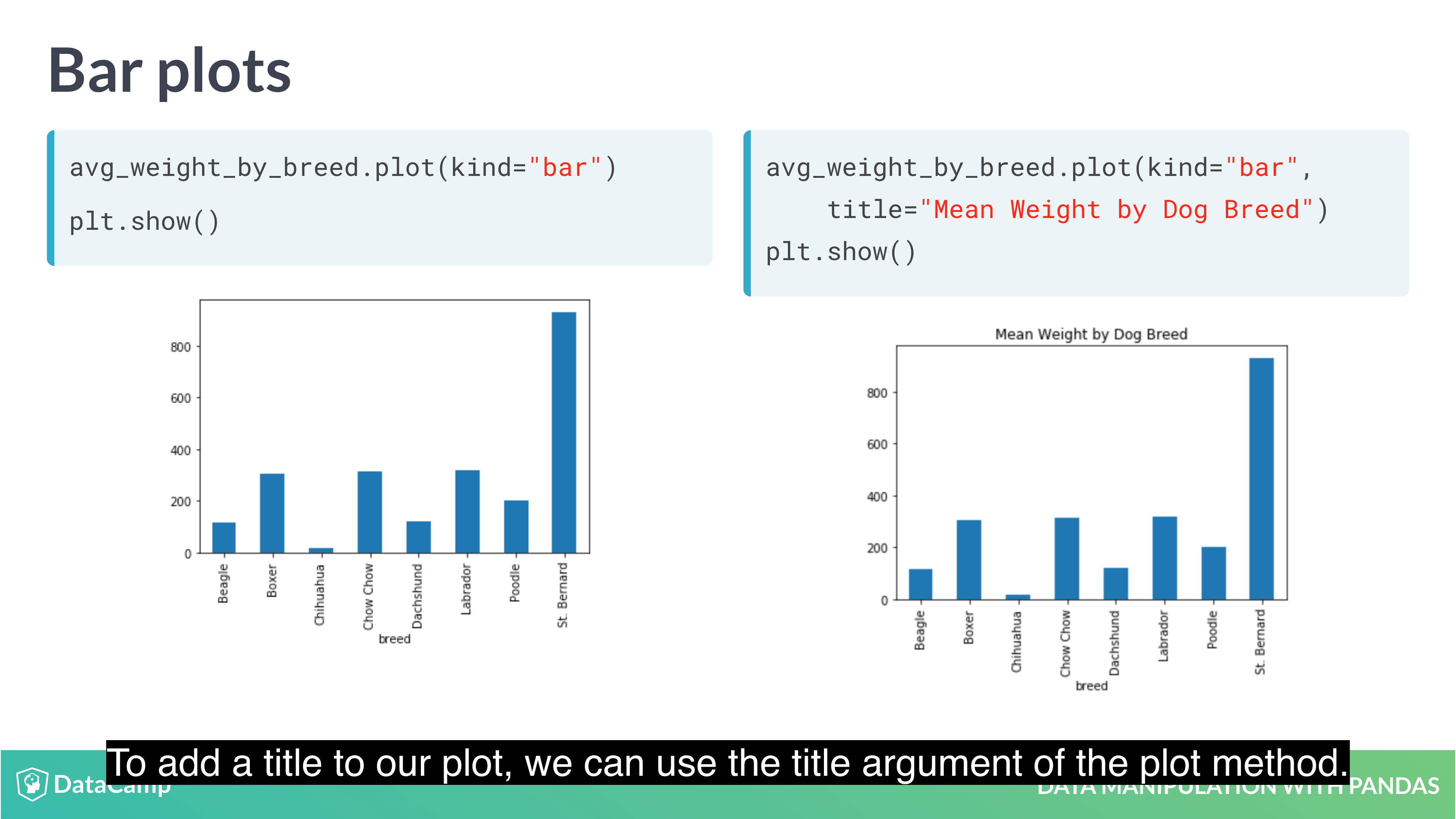
1 | # Bar Plot |
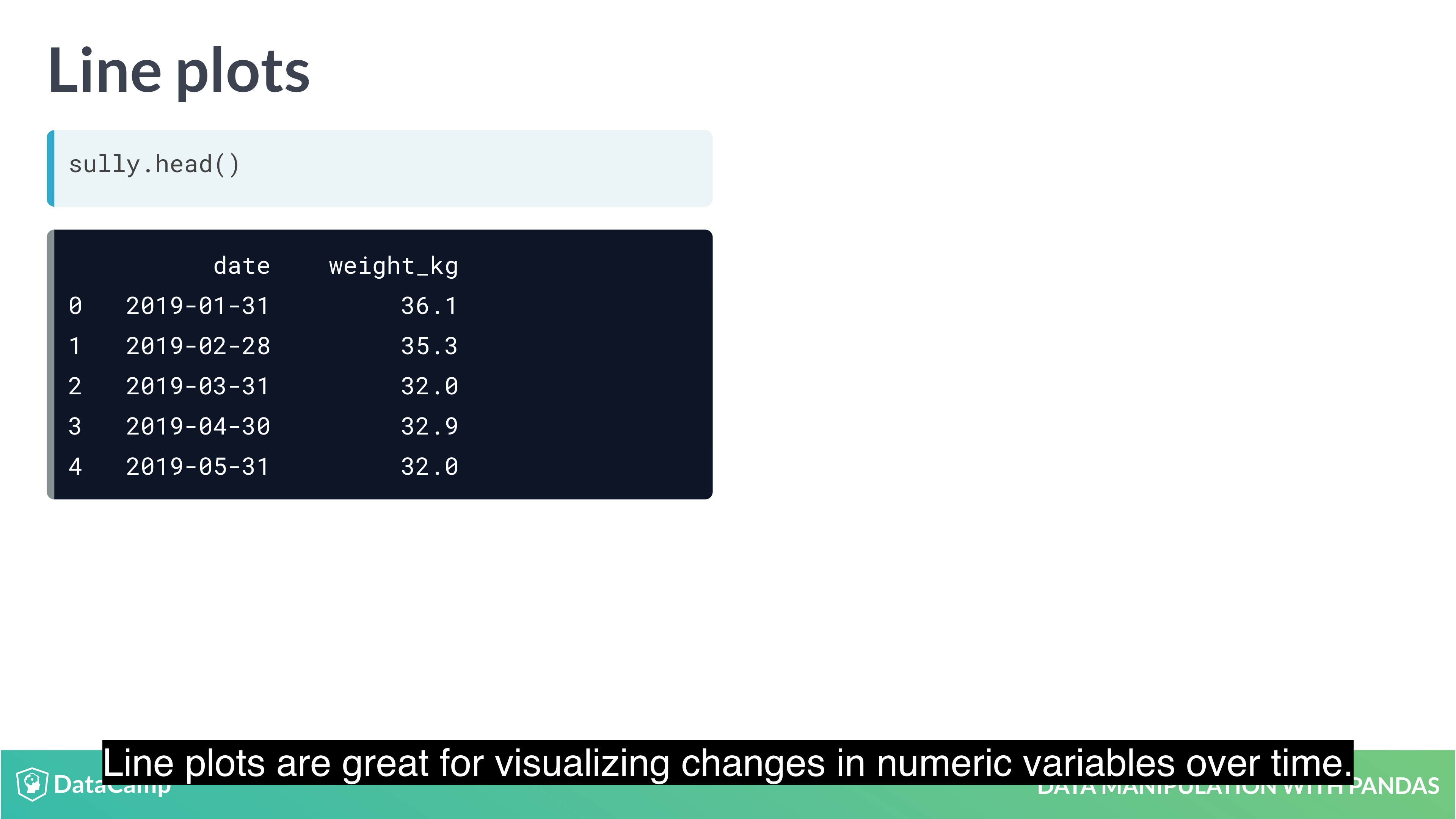
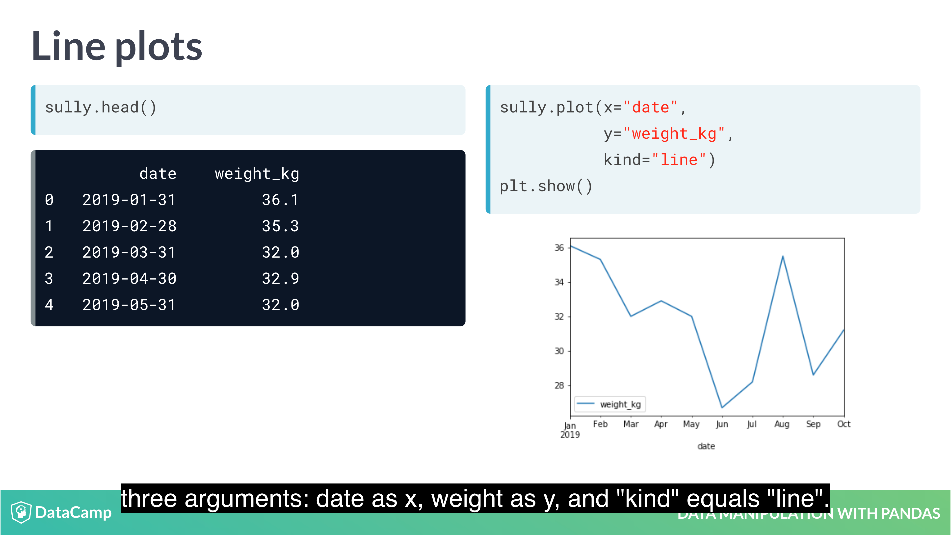
1 | # Line Plot |
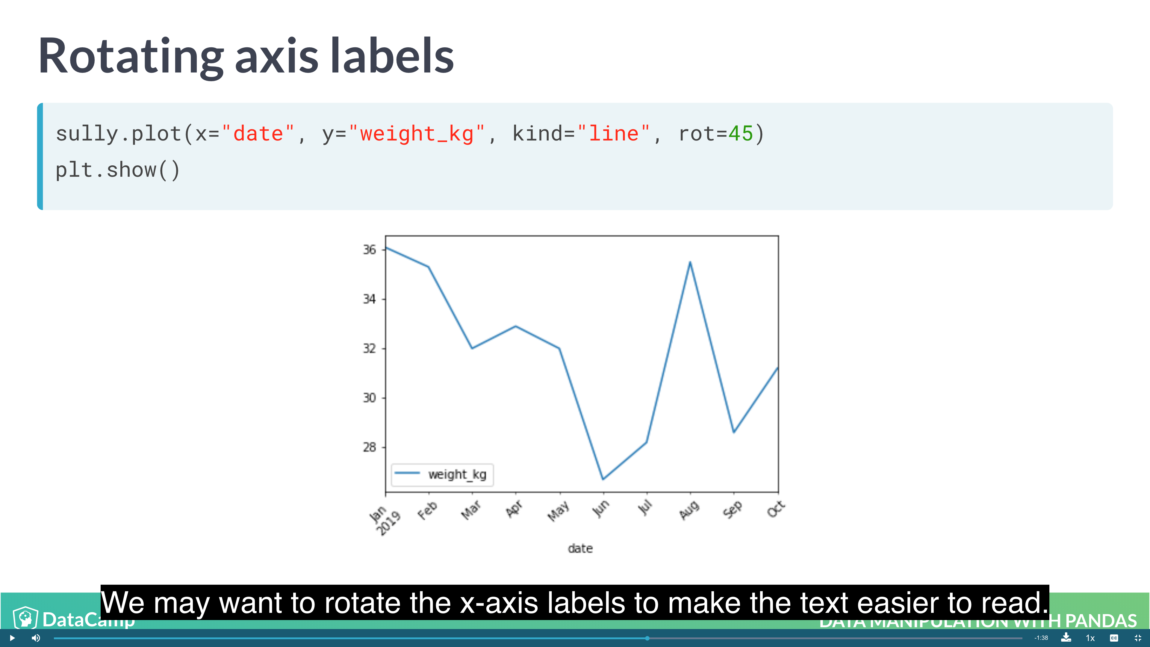
1 | # Rotating Axis Labels |
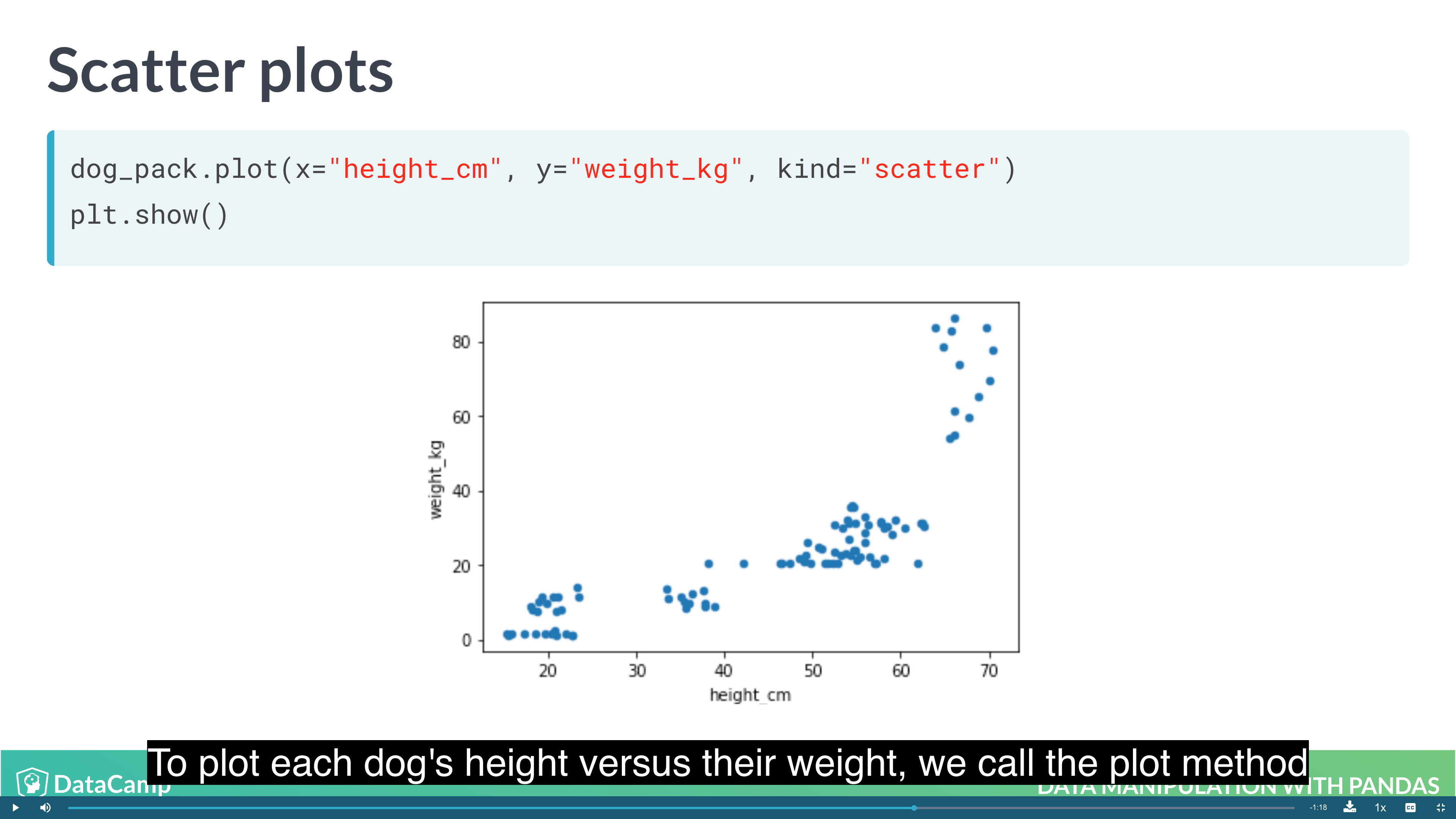
1 | # Scatter Plot |
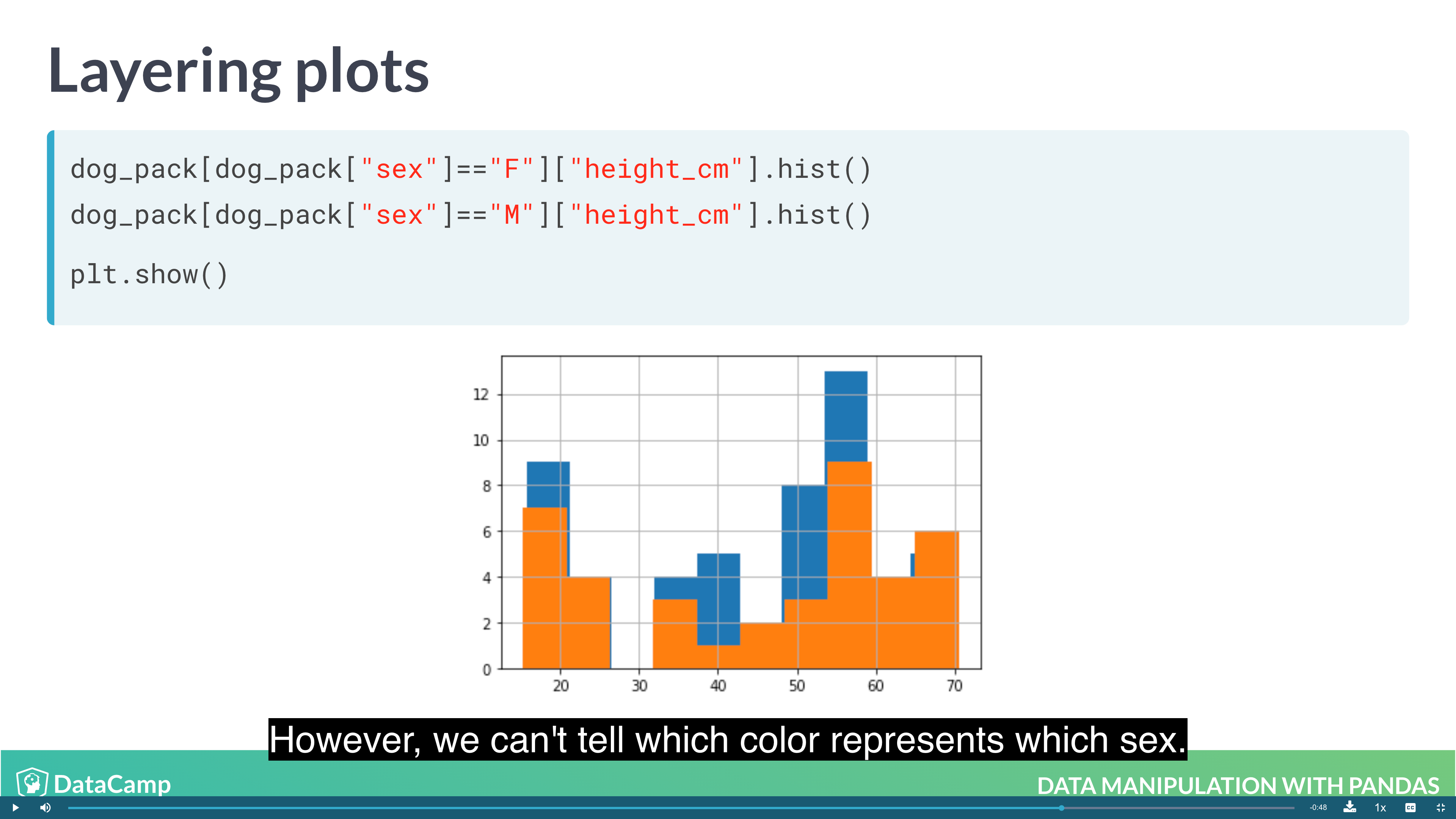
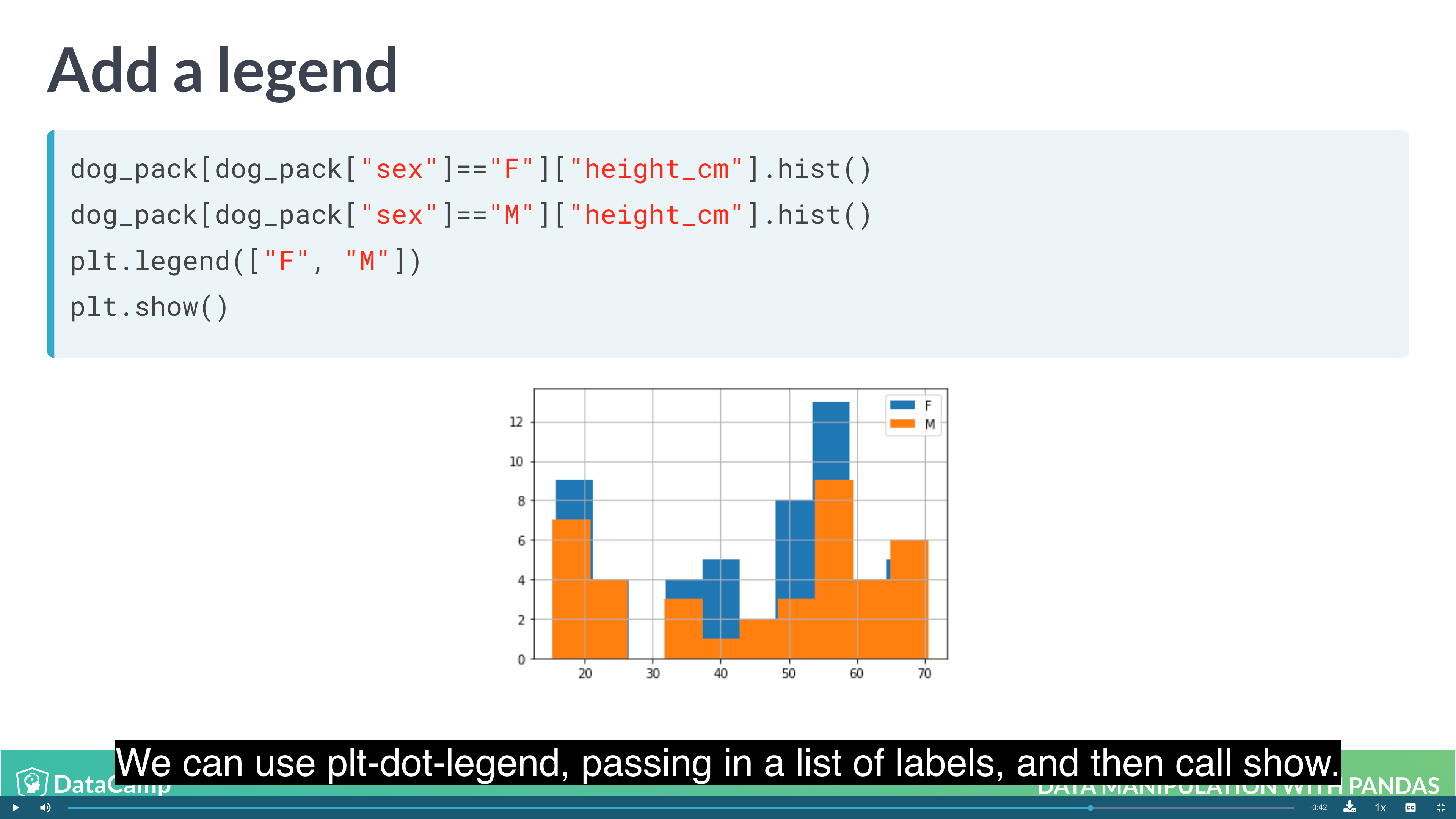
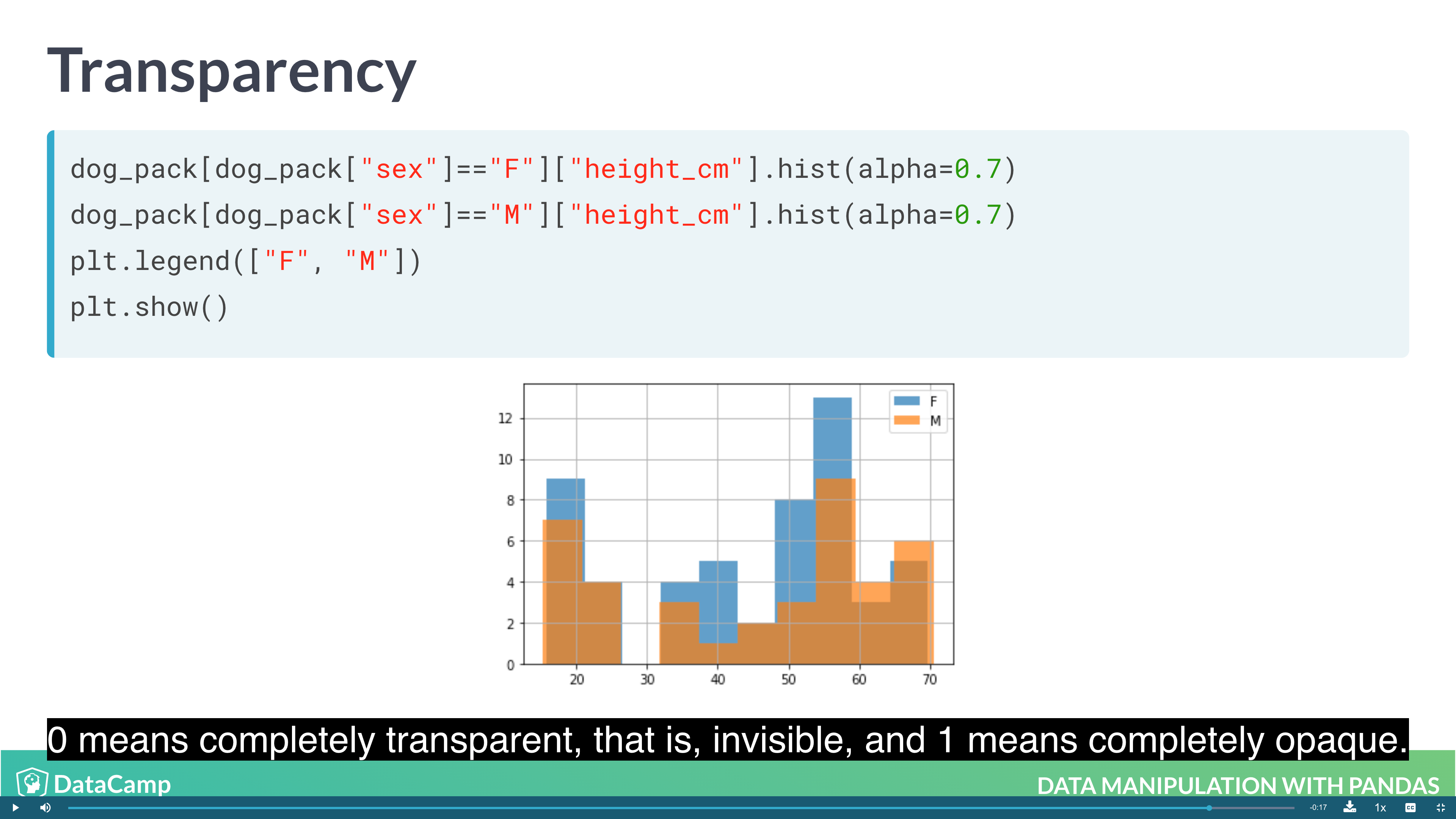
1 | # Layering Plot |
Example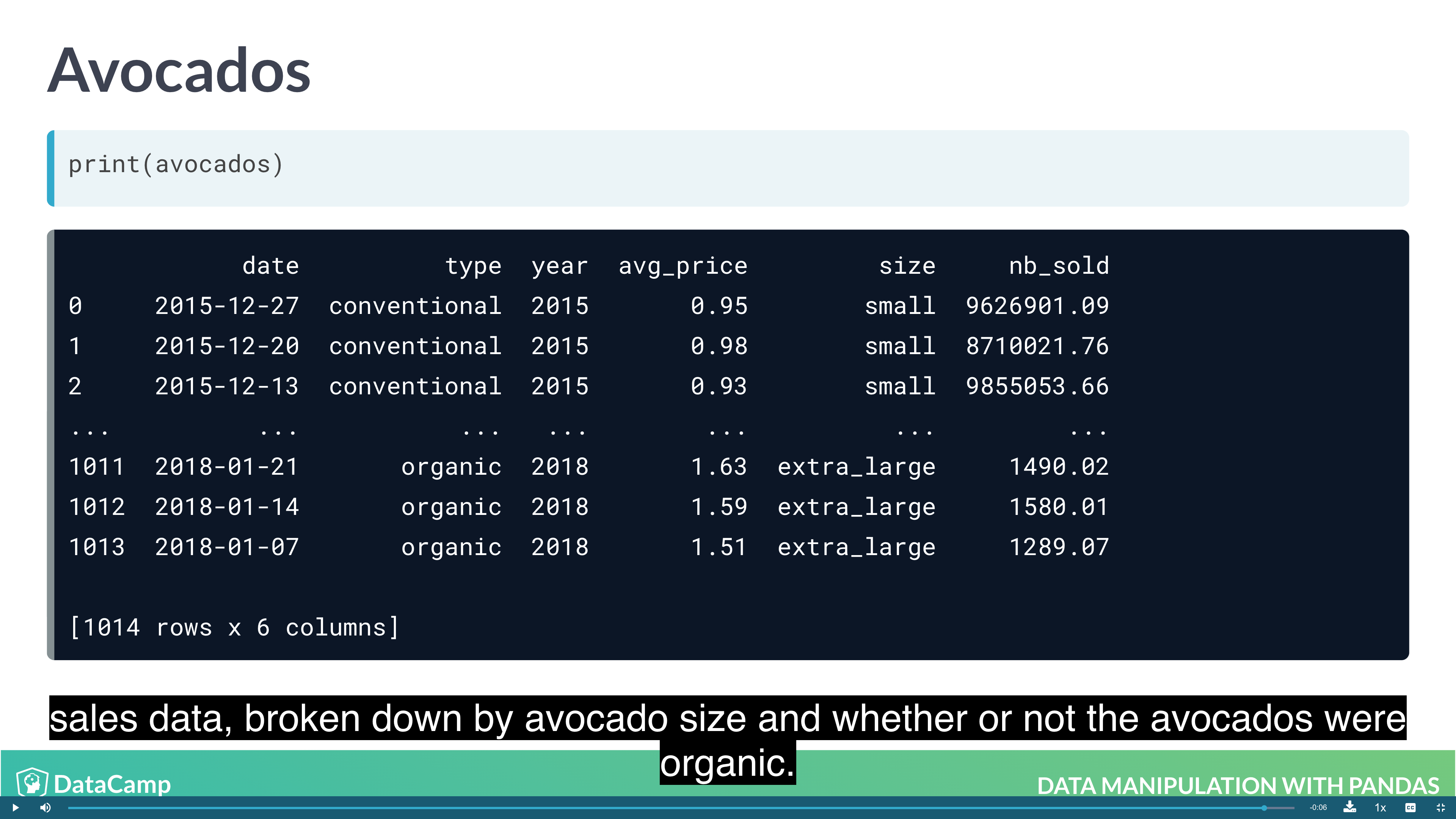
Missing Values
In a pandas DataFrame, missing values are indicated with NaN, which stands for “not a number”.
1 | df.isna() |
1 | df.dropna() # It is not ideal if you have a lot of missing values. |
1 | df.fillna(0) |
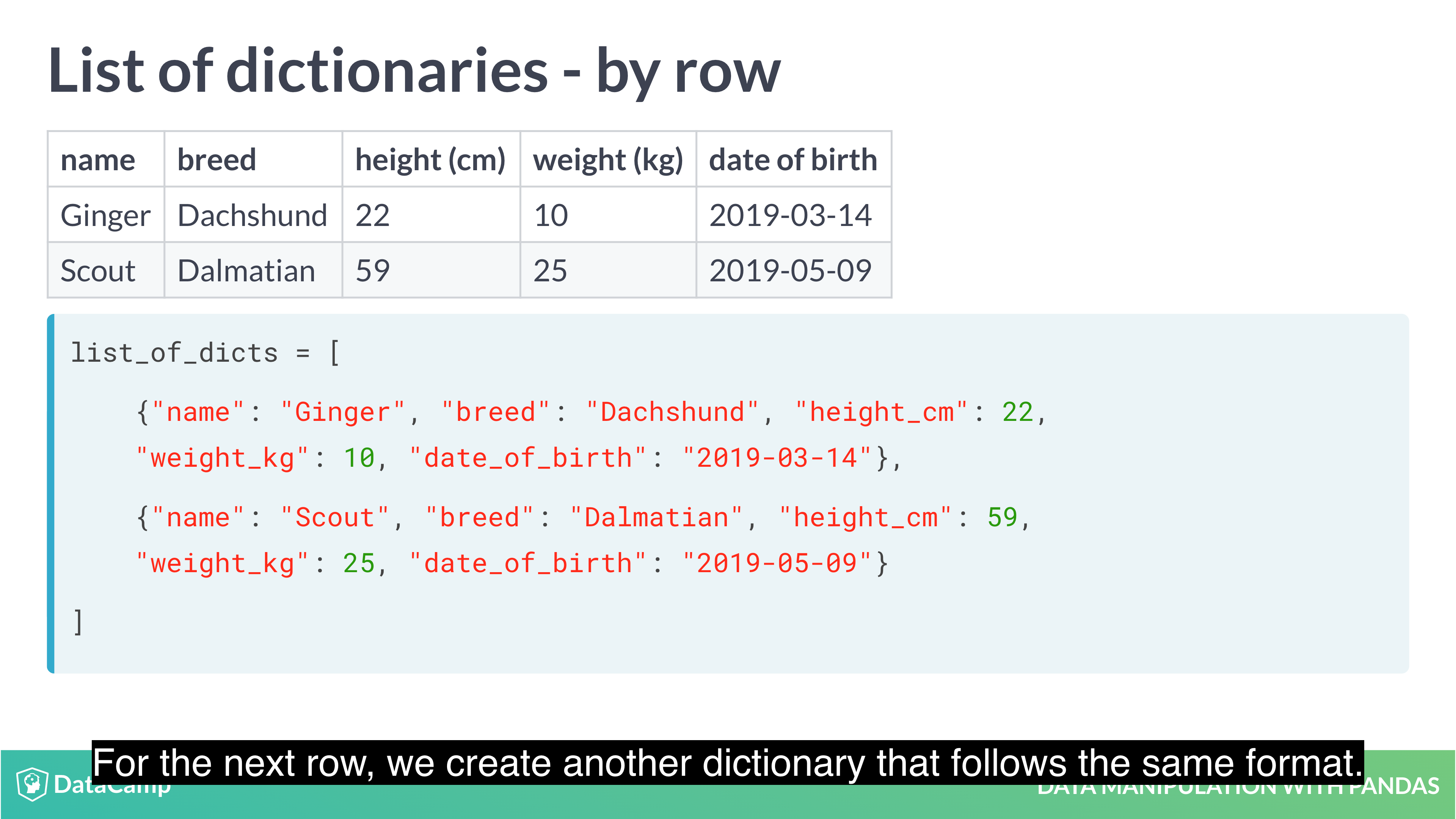
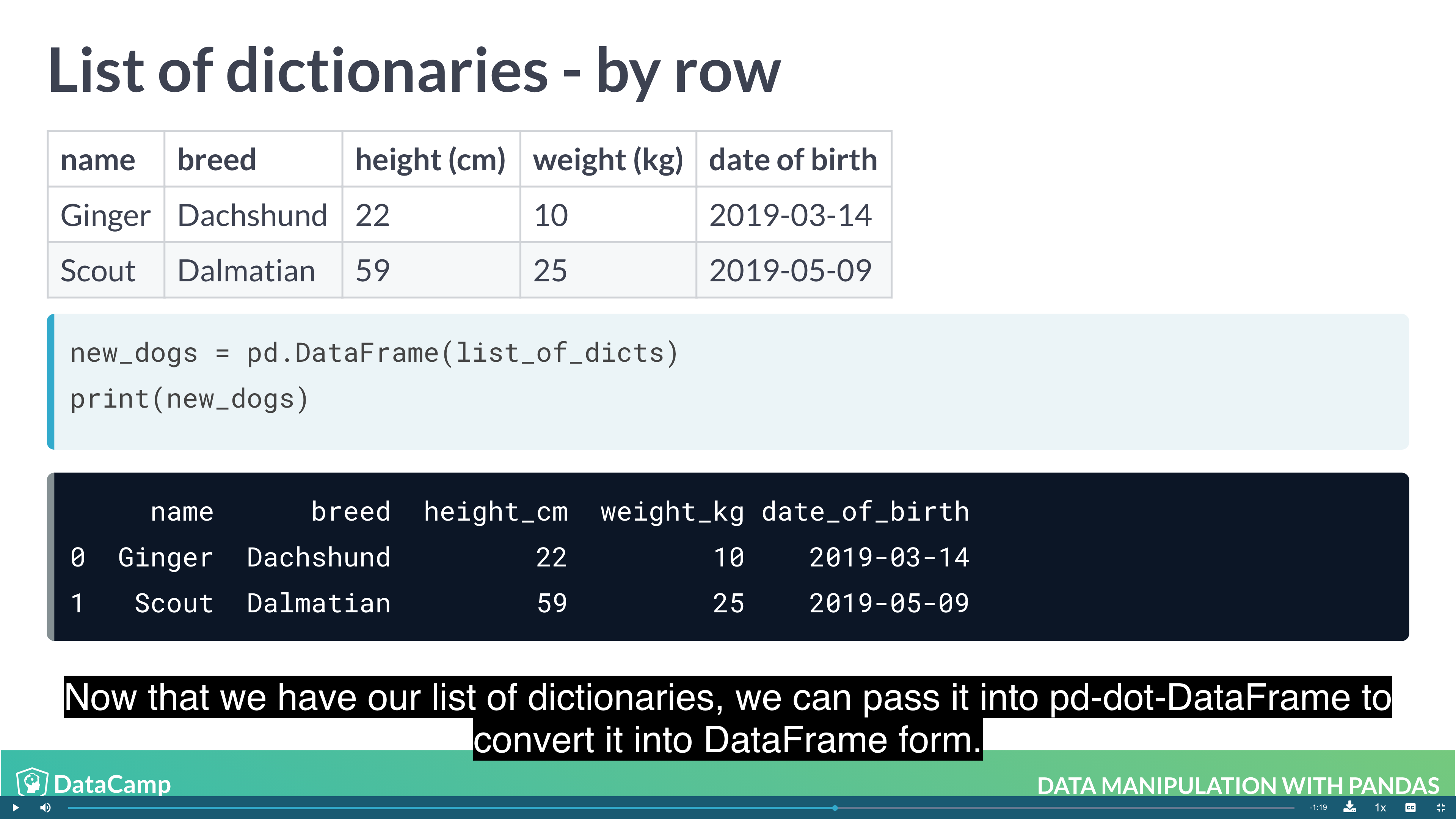
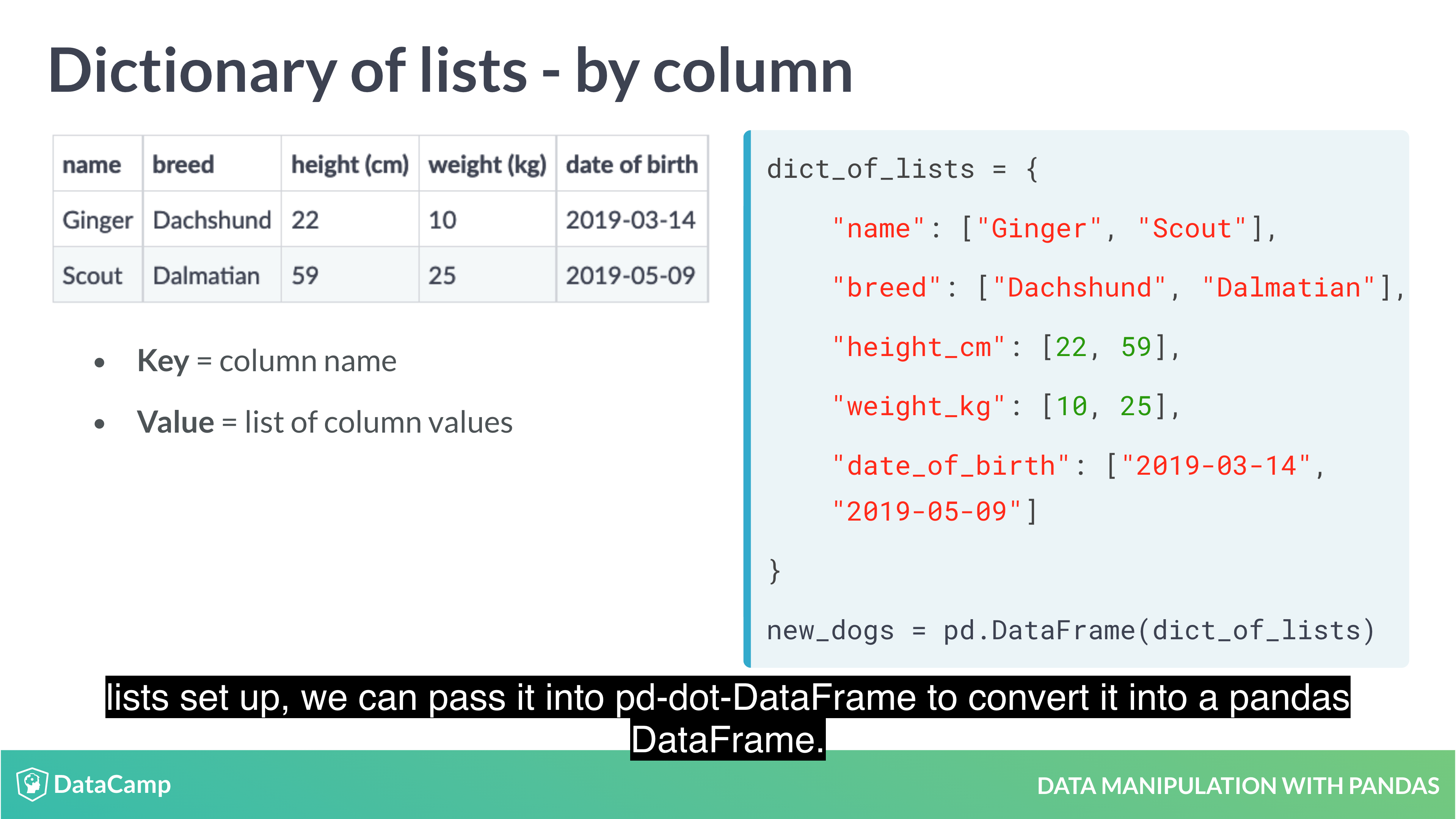
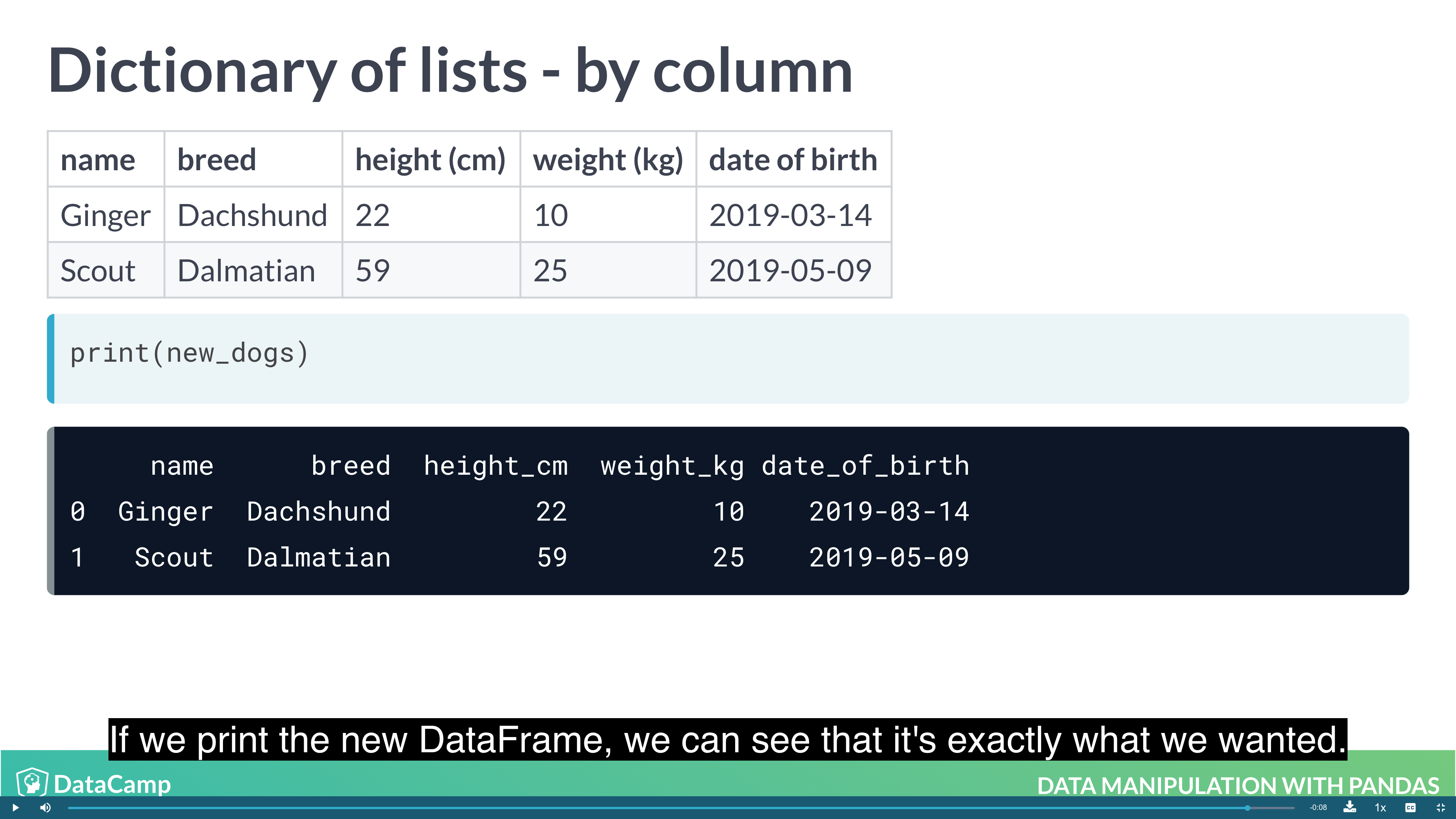
Creating DataFrames
Creating Dataframes:
- From a list of dictionaries: Constructed row by row
- From a dictionary of lists: Constructed column by column
1 | dic = { |
Creating DataFrames from List of Dictionaries
Creating DataFrames from Dictionary of lists
Reading and Writing CSVs
- CSV: Comma-Separated-Values.
- Designed for DataFrame-like data.
- Most database and spreadsheet programs can use them or create them.
1 | df = pd.read_csv("csv_file") |
More to Learn
- Merging DataFrames with Pandas
- Streamlined Data Ingestion with Pandas
- Analyzing Police Activity with Pandas
- Analyzing Marketing Campaigns with Pandas
One More Thing
Python Algorithms - Words: 2,640
Python Crawler - Words: 1,663
Python Data Science - Words: 4,551
Python Django - Words: 2,409
Python File Handling - Words: 1,533
Python Flask - Words: 874
Python LeetCode - Words: 9
Python Machine Learning - Words: 5,532
Python MongoDB - Words: 32
Python MySQL - Words: 1,655
Python OS - Words: 707
Python plotly - Words: 6,649
Python Quantitative Trading - Words: 353
Python Tutorial - Words: 25,451
Python Unit Testing - Words: 68