LearningSpark
Reference
Spark Features
Spark Purpose
In particular, data engineers will learn how to use Spark’s Structured APIs to perform complex data exploration and analysis on both batch and streaming data; use Spark SQL for interactive queries; use Spark’s built-in and external data sources to read, refine, and write data in different file formats as part of their extract, transform, and load (ETL) tasks; and build reliable data lakes with Spark and the open source Delta Lake table format.
Speed
Second, Spark builds its query computations as a directed acyclic graph (DAG); its DAG scheduler and query optimizer construct an efficient computational graph that can usually be decomposed into tasks that are executed in parallel across workers on the cluster
Ease of Use
Spark achieves simplicity by providing a fundamental abstraction of a simple logical data structure called a Resilient Distributed Dataset (RDD) upon which all other higher-level structured data abstractions, such as DataFrames and Datasets, are constructed.
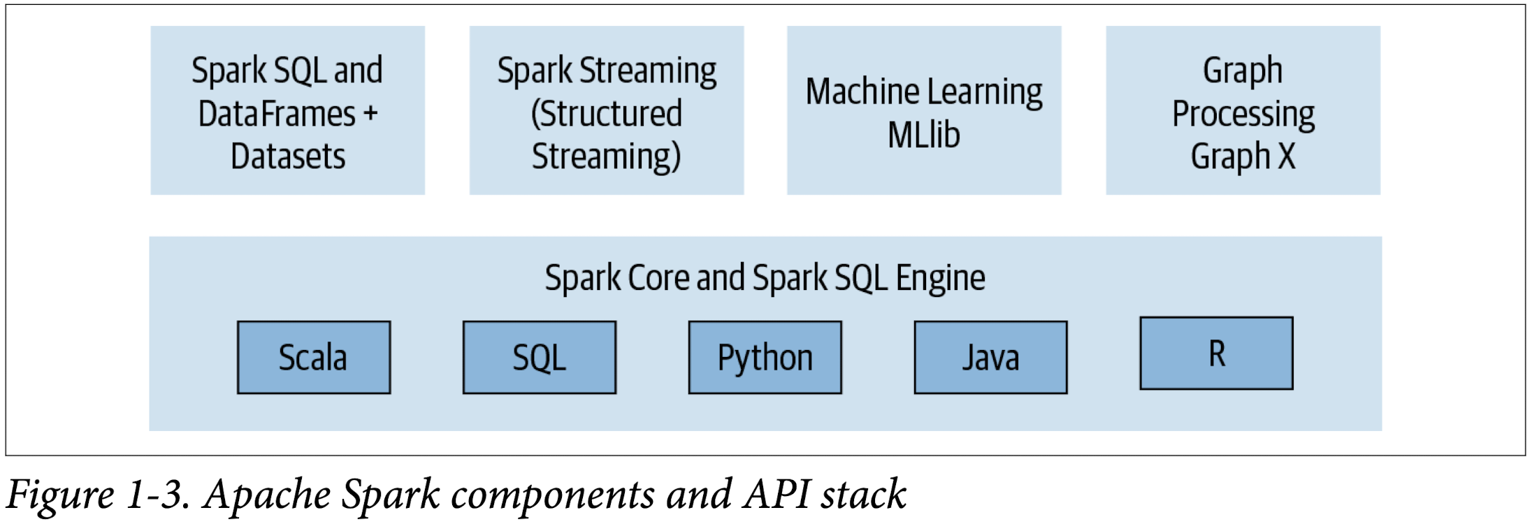
Modularity
Spark SQL, Spark Structured Streaming, Spark MLlib, and GraphX
Extensibiltiy
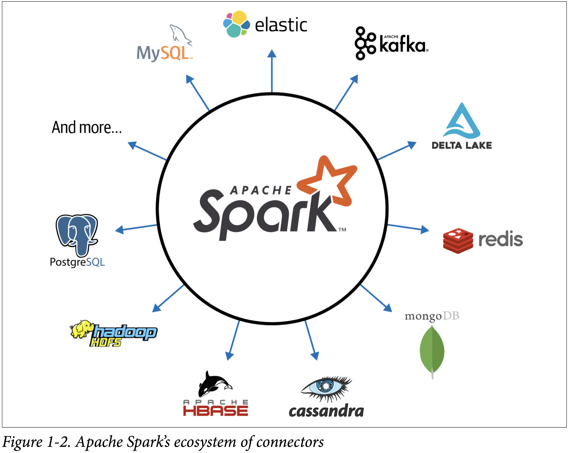
Spark to read data stored in myriad sources—Apache Hadoop, Apache Cassandra, Apache HBase, MongoDB, Apache Hive, RDBMSs, and more—and process it all in memory. Spark’s DataFrameReaders and DataFrame Writers can also be extended to read data from other sources, such as Apache Kafka, Kinesis, Azure Storage, and Amazon S3, into its logical data abstraction, on which it can operate.
Spark Components
Apache Spark’s Distributed Execution
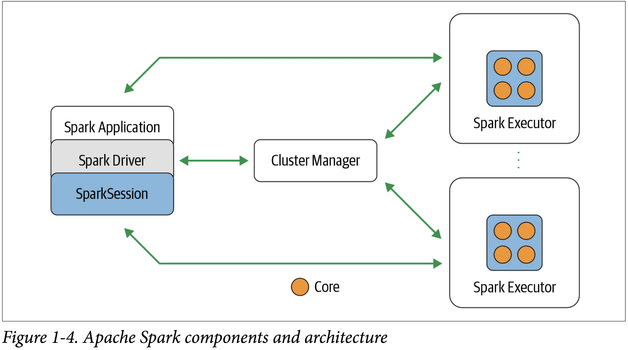
Spark driver
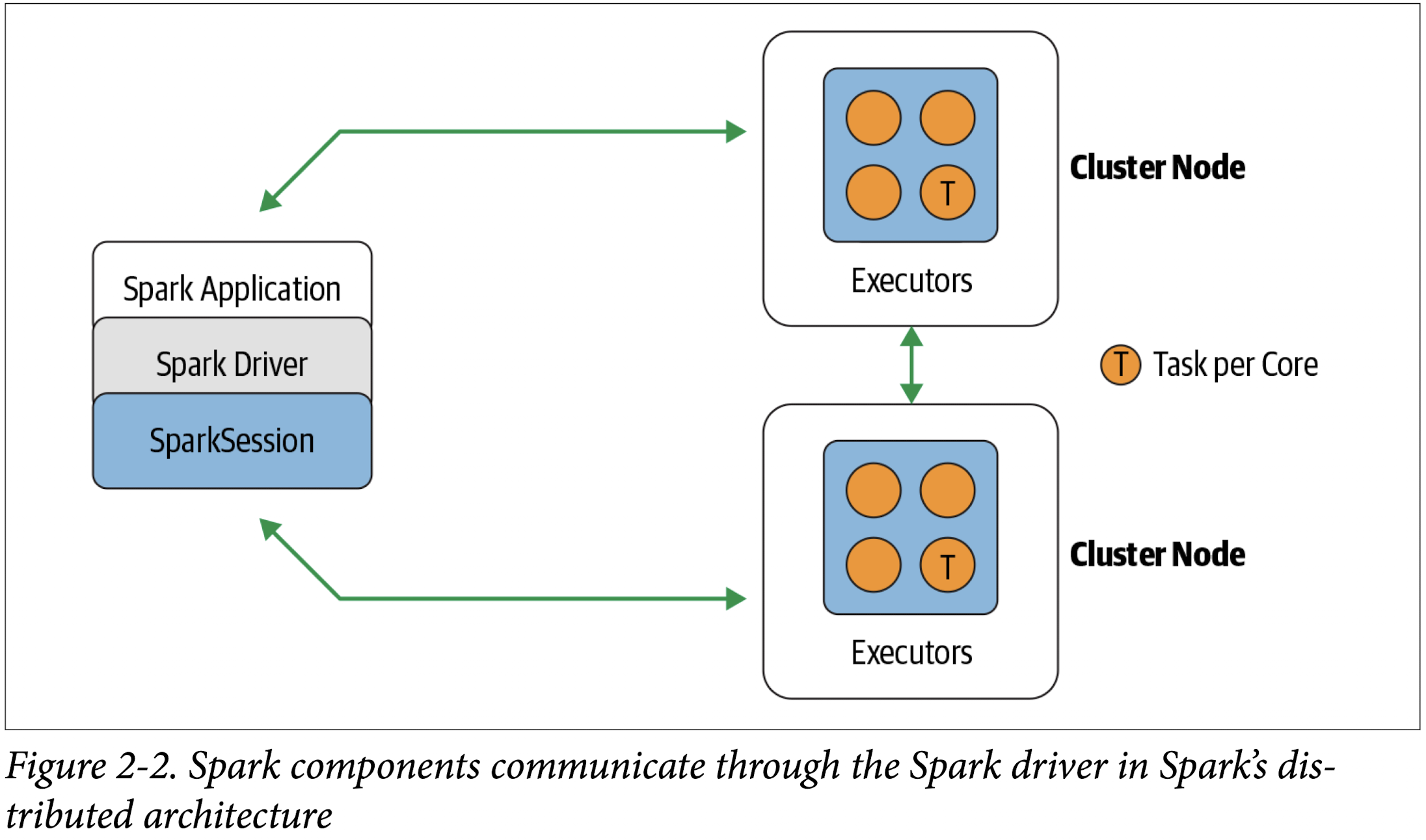
As the part of the Spark application responsible for instantiating a SparkSession, the Spark driver has multiple roles: it communicates with the cluster manager; it requests resources (CPU, memory, etc.) from the cluster manager for Spark’s executors (JVMs); and it transforms all the Spark operations into DAG computations, schedules them, and distributes their execution as tasks across the Spark executors. Once the resources are allocated, it communicates directly with the executors.
SparkSession
In Spark 2.0, the SparkSession became a unified conduit to all Spark operations and data. Not only did it subsume previous entry points to Spark like the SparkContext, SQLContext, HiveContext, SparkConf, and StreamingContext, but it also made working with Spark simpler and easier
Cluster manager
The cluster manager is responsible for managing and allocating resources for the cluster of nodes on which your Spark application runs. Currently, Spark supports four cluster managers: the built-in standalone cluster manager, Apache Hadoop YARN, Apache Mesos, and Kubernetes.
Spark executor
A Spark executor runs on each worker node in the cluster. The executors communicate with the driver program and are responsible for executing tasks on the workers. In most deployments modes, only a single executor runs per node.
Deployment methods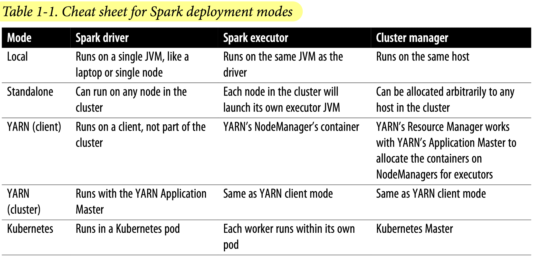
Distributed data and partitions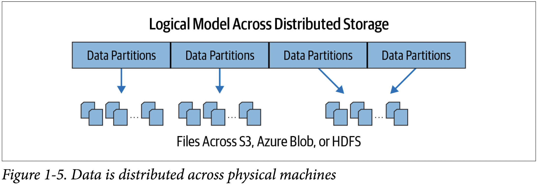
Spark Shell
1 | scala> val strings = spark.read.text("spark-3.2.1-bin-hadoop3.2/README.md") |
1 | strings = spark.read.text("spark-3.2.1-bin-hadoop3.2/README.md") |
1 | strings.show(10, truncate=True) |
Every computation expressed in high-level Structured APIs is decomposed into low-level optimized and generated RDD operations and then converted into Scala bytecode for the executors’ JVMs. This generated RDD operation code is not accessible to users, nor is it the same as the user-facing RDD APIs.
Spark Application
Spark Application Concepts
Application
- A user program built on Spark using its APIs. It consists of a driver program and executors on the cluster.
SparkSession
- An object that provides a point of entry to interact with underlying Spark functionality and allows programming Spark with its APIs. In an interactive Spark shell, the Spark driver instantiates a SparkSession for you, while in a Spark application, you create a SparkSession object yourself.
Job
- A parallel computation consisting of multiple tasks that gets spawned in response to a Spark action (e.g.,
save(),collect()).
Stage
- Each job gets divided into smaller sets of tasks called stages that depend on each other.
Task
- A single unit of work or execution that will be sent to a Spark executor.
Spark Application and SparkSession
At the core of every Spark application is the Spark driver program, which creates a SparkSession object. When you’re working with a Spark shell, the driver is part of the shell and the SparkSession object (accessible via the variable spark) is created for you, as you saw in the earlier examples when you launched the shells.
In those examples, because you launched the Spark shell locally on your laptop, all the operations ran locally, in a single JVM. But you can just as easily launch a Spark shell to analyze data in parallel on a cluster as in local mode. The commands spark-shell –help or pyspark –help will show you how to connect to the Spark cluster man‐ ager. Figure 2-2 shows how Spark executes on a cluster once you’ve done this.
Once you have a SparkSession, you can program Spark using the APIs to perform Spark operations.
Spark Jobs
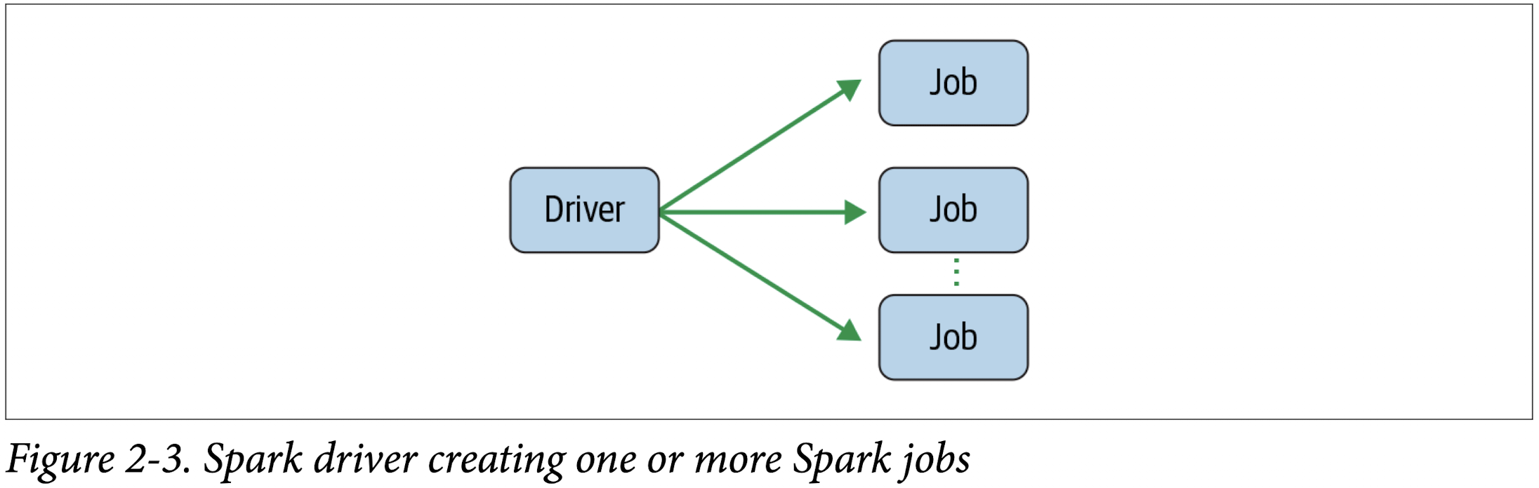
During interactive sessions with Spark shells, the driver converts your Spark applica‐ tion into one or more Spark jobs (Figure 2-3). It then transforms each job into a DAG. This, in essence, is Spark’s execution plan, where each node within a DAG could be a single or multiple Spark stages.
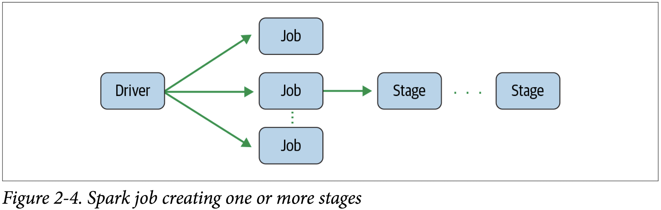
Spark Stage
As part of the DAG nodes, stages are created based on what operations can be per‐ formed serially or in parallel (Figure 2-4). Not all Spark operations can happen in a single stage, so they may be divided into multiple stages. Often stages are delineated on the operator’s computation boundaries, where they dictate data transfer among Spark executors.
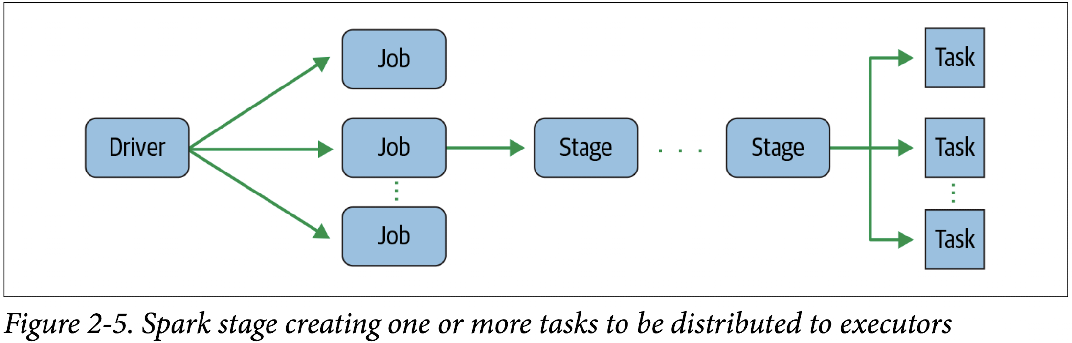
Spark Tasks
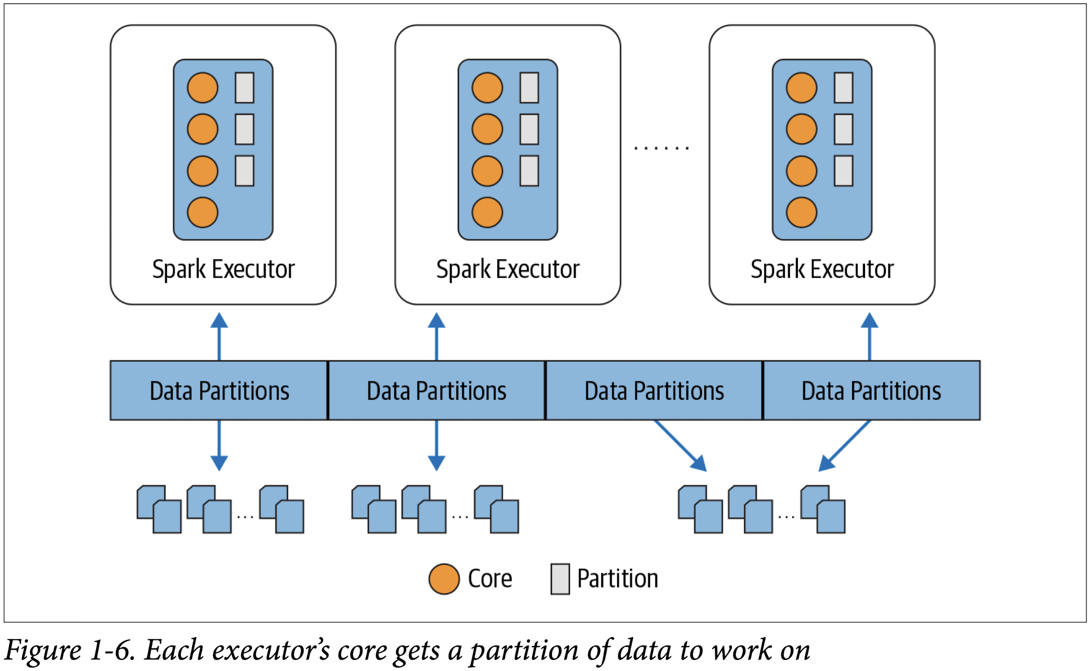
Each stage is comprised of Spark tasks (a unit of execution), which are then federated across each Spark executor; each task maps to a single core and works on a single par‐ tition of data (Figure 2-5). As such, an executor with 16 cores can have 16 or more tasks working on 16 or more partitions in parallel, making the execution of Spark’s tasks exceedingly parallel!
Transformations, Actions, and Lazy Evaluation
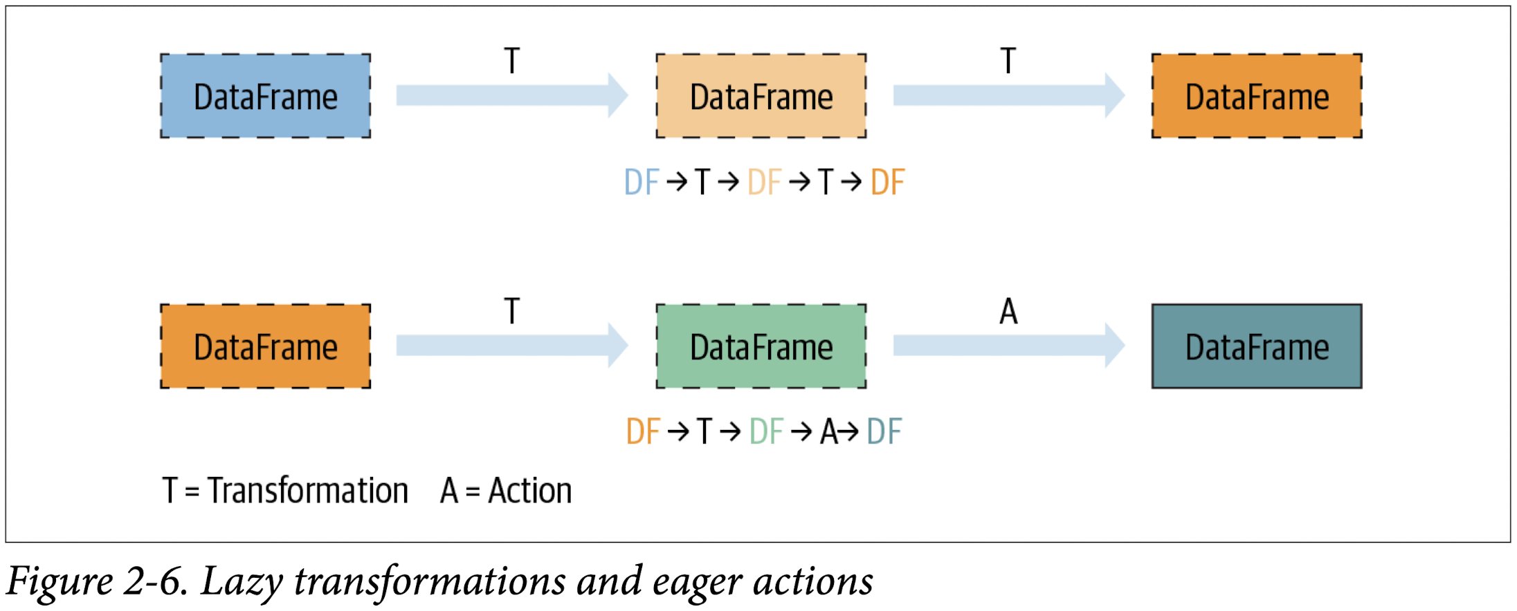
Spark operations on distributed data can be classified into two types: transformations and actions. Transformations, as the name suggests, transform a Spark DataFrame into a new DataFrame without altering the original data, giving it the property of immutability. Put another way, an operation such as select() or filter() will not change the original DataFrame; instead, it will return the transformed results of the operation as a new DataFrame.
All transformations are evaluated lazily. That is, their results are not computed immediately, but they are recorded or remembered as a lineage. A recorded lineage allows Spark, at a later time in its execution plan, to rearrange certain transformations, coalesce them, or optimize transformations into stages for more efficient execution. Lazy evaluation is Spark’s strategy for delaying execution until an action is invoked or data is “touched” (read from or written to disk).
An action triggers the lazy evaluation of all the recorded transformations. In
Figure 2-6, all transformations T are recorded until the action A is invoked. Each transformation T produces a new DataFrame.
While lazy evaluation allows Spark to optimize your queries by peeking into your chained transformations, lineage and data immutability provide fault tolerance. Because Spark records each transformation in its lineage and the DataFrames are immutable between transformations, it can reproduce its original state by simply replaying the recorded lineage, giving it resiliency in the event of failures.
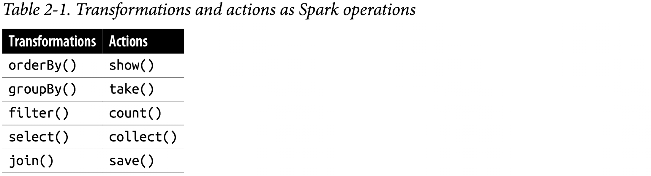
Table 2-1 lists some examples of transformations and actions.
Narrow and Wide Transformations
As noted, transformations are operations that Spark evaluates lazily. A huge advantage of the lazy evaluation scheme is that Spark can inspect your computational query and ascertain how it can optimize it. This optimization can be done by either joining or pipelining some operations and assigning them to a stage, or breaking them into stages by determining which operations require a shuffle or exchange of data across clusters.
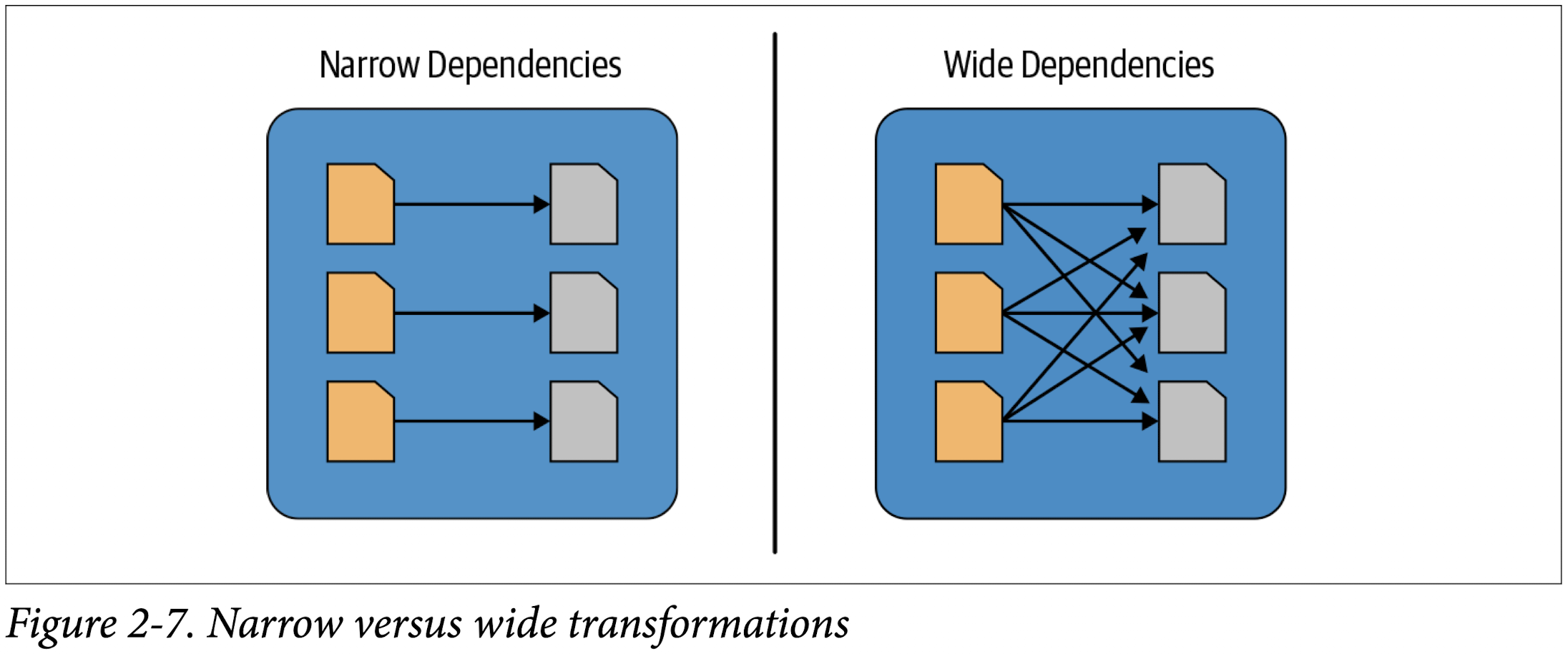
Transformations can be classified as having either narrow dependencies or wide dependencies. Any transformation where a single output partition can be computed from a single input partition is a narrow transformation. For example, in the previous code snippet, filter() and contains() represent narrow transformations because they can operate on a single partition and produce the resulting output partition without any exchange of data.
However, groupBy() or orderBy() instruct Spark to perform wide transformations, where data from other partitions is read in, combined, and written to disk. Since each partition will have its own count of the word that contains the “Spark” word in its row of data, a count (groupBy()) will force a shuffle of data from each of the executor’s partitions across the cluster. In this transformation, orderBy() requires output from other partitions to compute the final aggregation.
Figure 2-7 illustrates the two types of dependencies.
The Spark UI
Spark includes a graphical user interface that you can use to inspect or monitor Spark applications in their various stages of decomposition—that is jobs, stages, and tasks. Depending on how Spark is deployed, the driver launches a web UI, running by default on port 4040, where you can view metrics and details such as:
- A list of scheduler stages and tasks
- A summary of RDD sizes and memory usage
- Information about the environment
- Information about the running executors
- All the Spark SQL queries
In local mode, you can access this interface at http://<localhost>:4040 in a web browser.
Counting M&Ms for the Cookie Monster
Set environment variables
env– The command allows you to run another program in a custom environment without modifying the current one. When used without an argument it will print a list of the current environment variables.printenv– The command prints all or the specified environment variables.set– The command sets or unsets shell variables. When used without an argument it will print a list of all variables including environment and shell variables, and shell functions.unset– The command deletes shell and environment variables.export– The command sets environment variables./etc/environment- Use this file to set up system-wide environment variables./etc/profile- Variables set in this file are loaded whenever a bash login shell is entered. ```Per-user shell specific configuration files. For example, if you are using Bash, you can declare the variables in the
~/.bashrc:
Set your SPARK_HOME environment variable to the root-level directory where you installed Spark on your local machine.
1 | ➜ spark-3.2.1-bin-hadoop3.2 pwd |
1 | ➜ spark-3.2.1-bin-hadoop3.2 echo 'export SPARK_HOME="/Users/zacks/Git/Data Science Projects/spark-3.2.1-bin-hadoop3.2"' >> ~/.zshrc |
Review ~/.zshrc
1 | ➜ spark-3.2.1-bin-hadoop3.2 tail -1 ~/.zshrc |
To avoid having verbose INFO messages printed to the console, copy the log4j.properties.template file to log4j.properties and set log4j.rootCategory=WARN in the conf/log4j.properties file.
Content in log4j.properties.template
1 | ➜ spark-3.2.1-bin-hadoop3.2 cat conf/log4j.properties.template |
1 | ➜ spark-3.2.1-bin-hadoop3.2 cp conf/log4j.properties.template conf/log4j.properties |
After edit log4j.rootCategory in log4j.properties
1 | ➜ spark-3.2.1-bin-hadoop3.2 cat conf/log4j.properties | grep log4j.rootCategory |
Spark Job
Under LearningSparkV2/chapter2/py/src
1 | ➜ src git:(dev) ✗ source ~/.zshrc |
Output:
1st table: head of df
2nd table: sum Count group by State, Color
3rd table: sum Count group by State, Color where Color = 'CA'
1 | WARNING: An illegal reflective access operation has occurred |
Spark’s Structured APIs
Spark: What’s Underneath an RDD?
The RDD is the most basic abstraction in Spark. There are three vital characteristics associated with an RDD:
- Dependencies
- Partitions (with some locality information)
- Compute function: Partition =>
Iterator[T]
All three are integral to the simple RDD programming API model upon which all higher-level functionality is constructed. First, a list of dependencies that instructs Spark how an RDD is constructed with its inputs is required. When necessary to reproduce results, Spark can recreate an RDD from these dependencies and replicate operations on it. This characteristic gives RDDs resiliency.
Second, partitions provide Spark the ability to split the work to parallelize computation on partitions across executors. In some cases—for example, reading from HDFS—Spark will use locality information to send work to executors close to the data. That way less data is transmitted over the network.
And finally, an RDD has a compute function that produces an Iterator[T] for the data that will be stored in the RDD.
Structuring Spark
Key Metrics and Benefits
Structure yields a number of benefits, including better performance and space efficiency across Spark components. We will explore these benefits further when we talk about the use of the DataFrame and Dataset APIs shortly, but for now we’ll concentrate on the other advantages: expressivity, simplicity, composability, and uniformity.
Let’s demonstrate expressivity and composability first, with a simple code snippet. In the following example, we want to aggregate all the ages for each name, group by name, and then average the ages—a common pattern in data analysis and discovery. If we were to use the low-level RDD API for this, the code would look as follows:
1 | # In Python |
No one would dispute that this code, which tells Spark how to aggregate keys and compute averages with a string of lambda functions, is cryptic and hard to read. In other words, the code is instructing Spark how to compute the query. It’s completely opaque to Spark, because it doesn’t communicate the intention. Furthermore, the equivalent RDD code in Scala would look very different from the Python code shown here.
By contrast, what if we were to express the same query with high-level DSL operators and the DataFrame API, thereby instructing Spark what to do? Have a look:
1 | # In Python |
The DataFrame API
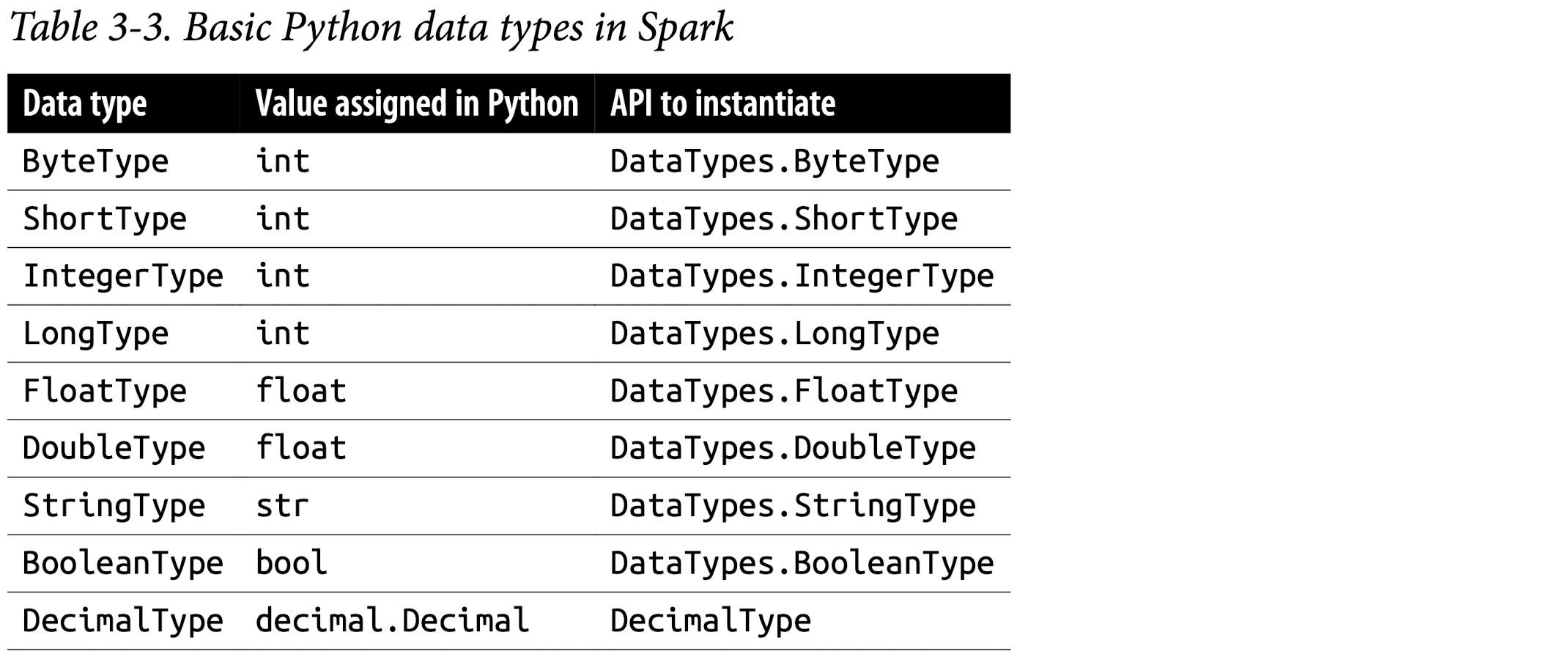
Spark’s Basic Data Types
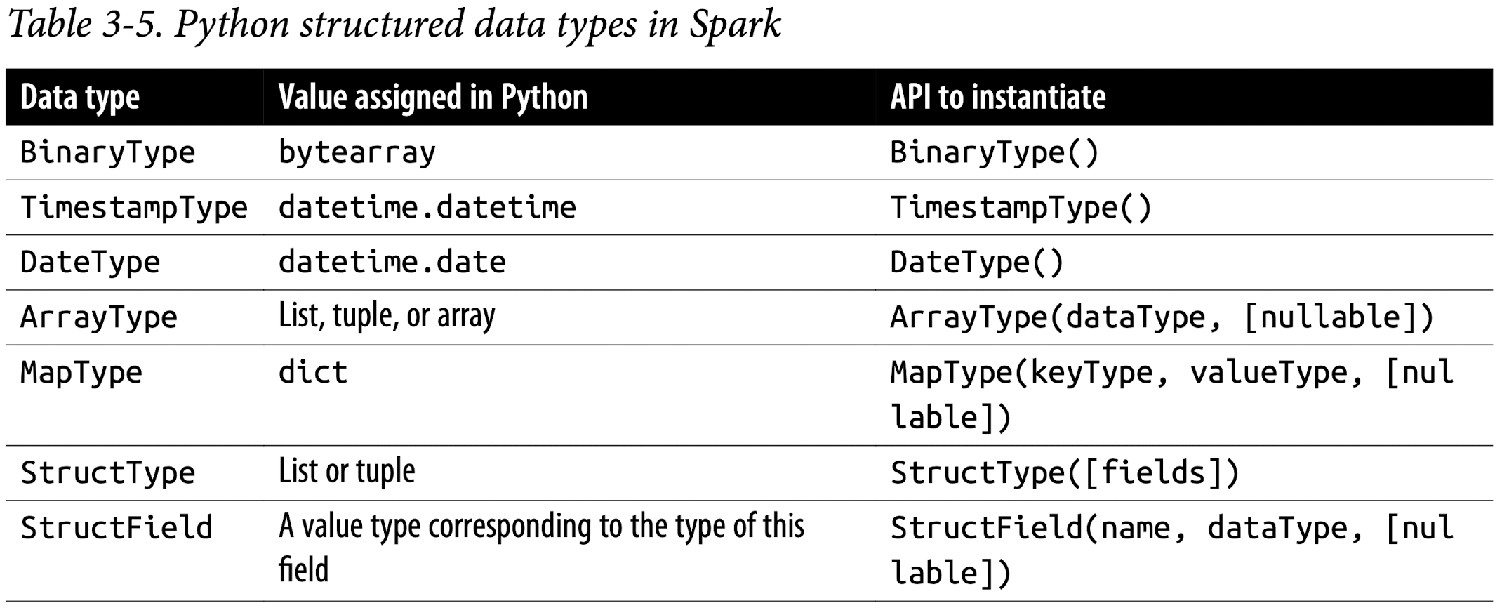
Spark’s Structured and Complex Data Types
Schemas and Creating DataFrames
A schema in Spark defines the column names and associated data types for a DataFrame.
Defining a schema up front as opposed to taking a schema-on-read approach offers three benefits:
- You relieve Spark from the onus of inferring data types.
- You prevent Spark from creating a separate job just to read a large portion of your file to ascertain the schema, which for a large data file can be expensive and time-consuming.
- You can detect errors early if data doesn’t match the schema.
So, we encourage you to always define your schema up front whenever you want to read a large file from a data source.
Two ways to define a schema
Spark allows you to define a schema in two ways. One is to define it programmatically, and the other is to employ a Data Definition Language (DDL) string, which is much simpler and easier to read.
To define a schema programmatically for a DataFrame with three named columns, author, title, and pages, you can use the Spark DataFrame API. For example:
1 | # In Python |
Defining the same schema using DDL is much simpler:
1 | # In Python |
You can choose whichever way you like to define a schema. For many examples, we will use both:
1 | # define schema by using Spark DataFrame API |
1 | # define schema by using Definition Language (DDL) |
Columns and Expressions
Named columns in DataFrames are conceptually similar to named columns in pandas or R DataFrames or in an RDBMS table: they describe a type of field. You can list all the columns by their names, and you can perform operations on their values using relational or computational expressions. In Spark’s supported languages, columns are objects with public methods (represented by the Column type).
You can also use logical or mathematical expressions on columns. For example, you could create a simple expression using expr("columnName * 5") or (expr("columnName - 5") > col(anothercolumnName)), where columnName is a Spark type (integer, string, etc.). expr() is part of the pyspark.sql.functions (Python) and org.apache.spark.sql.functions (Scala) packages. Like any other function in those packages, expr() takes arguments that Spark will parse as an expression, computing the result.
Scala, Java, and Python all have public methods associated with columns. You’ll note that the Spark documentation refers to both
colandColumn. Column is the name of the object, whilecol()is a standard built-in function that returns aColumn.
We have only scratched the surface here, and employed just a couple of methods on Column objects. For a complete list of all public methods for
Columnobjects, we refer you to the Spark documentation.
Column objects in a DataFrame can’t exist in isolation; each column is part of a row in a record and all the rows together constitute a DataFrame, which as we will see later in the chapter is really a Dataset[Row] in Scala.
Rows
A row in Spark is a generic Row object, containing one or more columns. Each column may be of the same data type (e.g., integer or string), or they can have different types (integer, string, map, array, etc.). Because Row is an object in Spark and an ordered collection of fields, you can instantiate a Row in each of Spark’s supported languages and access its fields by an index starting at 0:
1 | from pyspark.sql import Row |
Row objects can be used to create DataFrames if you need them for quick interactivity and exploration:
1 | rows = [Row("Matei Zaharia", "CA"), Row("Reynold Xin", "CA")] |
Common DataFrame Operations
To perform common data operations on DataFrames, you’ll first need to load a Data‐ Frame from a data source that holds your structured data. Spark provides an inter‐ face, DataFrameReader, that enables you to read data into a DataFrame from myriad data sources in formats such as JSON, CSV, Parquet, Text, Avro, ORC, etc. Likewise, to write a DataFrame back to a data source in a particular format, Spark uses DataFrameWriter.
Using DataFrameReader and DataFrameWriter
By defining a schema and use DataFrameReader class and its methods to tell Spark what to do, it’s more efficient to define a schema than have Spark infer it.
inferSchema
If you don’t want to specify the schema, Spark can infer schema from a sample at a lesser cost. For example, you can use the samplingRatio option(under chapter3 directory):
1 | sampleDF = (spark |
The following example shows how to read DataFrame with a schema:
1 | from pyspark.sql.types import * |
The spark.read.csv() function reads in the CSV file and returns a DataFrame of rows and named columns with the types dictated in the schema.
To write the DataFrame into an external data source in your format of choice, you can use the DataFrameWriter interface. Like DataFrameReader, it supports multiple data sources. Parquet, a popular columnar format, is the default format; it uses snappy compression to compress the data. If the DataFrame is written as Parquet, the schema is preserved as part of the Parquet metadata. In this case, subsequent reads back into a DataFrame do not require you to manually supply a schema.
Saving a DataFrame as a Parquet file or SQL table. A common data operation is to explore and transform your data, and then persist the DataFrame in Parquet format or save it as a SQL table. Persisting a transformed DataFrame is as easy as reading it. For exam‐ ple, to persist the DataFrame we were just working with as a file after reading it you would do the following:
1 | # In Python to save as Parquet files |
Alternatively, you can save it as a table, which registers metadata with the Hive metastore (we will cover SQL managed and unmanaged tables, metastores, and Data-Frames in the next chapter):
1 | # In Python to save as a Hive metastore |
Transformations and actions
Projections and filters
Projections and filters. A projection in relational parlance is a way to return only the rows matching a certain relational condition by using filters. In Spark, projections are done with the select() method, while filters can be expressed using the filter() or where() method. We can use this technique to examine specific aspects of our SF Fire Department data set:
1 | fire_parquet.select("IncidentNumber", "AvailableDtTm", "CallType") \ |
1 | +--------------+----------------------+-----------------------------+ |
What if we want to know how many distinct CallTypes were recorded as the causes of the fire calls? These simple and expressive queries do the job:
1 | (fire_parquet |
1 | +-----------------+ |
We can list the distinct call types in the data set using these queries:
1 | # In Python, filter for only distinct non-null CallTypes from all the rows |
Renaming, adding, and dropping columns
Renaming, adding, and dropping columns. Sometimes you want to rename particular columns for reasons of style or convention, and at other times for readability or brevity. The original column names in the SF Fire Department data set had spaces in them. For example, the column name IncidentNumber was Incident Number. Spaces in column names can be problematic, especially when you want to write or save a DataFrame as a Parquet file (which prohibits this).
By specifying the desired column names in the schema with StructField, as we did, we effectively changed all names in the resulting DataFrame.
Alternatively, you could selectively rename columns with the withColumnRenamed() method. For instance, let’s change the name of our Delay column to ResponseDelayedinMins and take a look at the response times that were longer than five minutes:
1 | # create a new dataframe new_fire_parquet from fire_parquet |
1 | +---------------------+ |
Because DataFrame transformations are immutable, when we rename a column using
withColumnRenamed()we get a new DataFrame while retaining the original with the old column name.
Modifying the contents of a column or its type are common operations during data exploration. In some cases the data is raw or dirty, or its types are not amenable to being supplied as arguments to relational operators. For example, in our SF Fire Department data set, the columns CallDate, WatchDate, and AlarmDtTm are strings rather than either Unix timestamps or SQL dates, both of which Spark supports and can easily manipulate during transformations or actions (e.g., during a date- or time- based analysis of the data).
So how do we convert them into a more usable format? It’s quite simple, thanks to some high-level API methods. spark.sql.functions has a set of to/from date/timestamp functions such as to_timestamp() and to_date() that we can use for just this purpose:
1 | # transform CallDate from "MM/dd/yyyy" to timestamp with name IncidentDate and drop CallDate |
- Convert the existing column’s data type from string to a Spark-supported timestamp.
- Use the new format specified in the format string “MM/dd/yyyy” or “MM/dd/yyyy hh:mm:ss a” where appropriate.
- After converting to the new data type,
drop()the old column and append the new one specified in the first argument to thewithColumn()method. - Assign the new modified DataFrame to
fire_ts_parquet.
1 | +-------------------+-------------------+-------------------+ |
Now that we have modified the dates, we can query using functions from spark.sql.functions like month(), year(), and day() to explore our data further. We could find out how many calls were logged in the last seven days, or we could see how many years’ worth of Fire Department calls are included in the data set with this query:
1 | # select distinct year(IncidentDate) from fire_ts_parquet order by 1 |
1 | +------------------+ |
Aggregations
A handful of transformations and actions on DataFrames, such as groupBy(), orderBy(), and count(), offer the ability to aggregate by column names and then aggregate counts across them.
For larger DataFrames on which you plan to conduct frequent or repeated queries, you could benefit from caching. We will cover DataFrame caching strategies and their benefits in later chapters.
1 | # select CallType, count(*) as `count` from fire_ts_parquet where CallType is not null group by CallType |
1 | +-------------------------------+------+ |
The DataFrame API also offers the
collect()method, but for extremely large DataFrames this is resource-heavy (expensive) and dangerous, as it can cause out-of-memory (OOM) exceptions. Unlikecount(), which returns a single number to the driver,collect()returns a collection of all the Row objects in the entire DataFrame or Dataset. If you want to take a peek at someRowrecords you’re better off withtake(n), which will return only the firstn Rowobjects of the DataFrame.
Other common DataFrame operations
Other common DataFrame operations. Along with all the others we’ve seen, the Data‐ Frame API provides descriptive statistical methods like min(), max(), sum(), and avg(). Let’s take a look at some examples showing how to compute them with our SF Fire Department data set.
Here we compute the sum of alarms, the average response time, and the minimum and maximum response times to all fire calls in our data set, importing the PySpark functions in a Pythonic way so as not to conflict with the built-in Python functions:
1 | import pyspark.sql.functions as F |
1 | +--------------+--------------------------+--------------------------+--------------------------+ |
For more advanced statistical needs common with data science workloads, read the API documentation for methods like stat(), describe(), correlation(), covariance(), sampleBy(), approxQuantile(), frequentItems(), and so on.
As you can see, it’s easy to compose and chain expressive queries with DataFrames’ high-level API and DSL operators. We can’t imagine the opacity and comparative unreadability of the code if we were to try to do the same with RDDs!
End-to-End DataFrame example
There are many possibilities for exploratory data analysis, ETL, and common data operations on the San Francisco Fire Department public data set, above and beyond what we’ve shown here.
For brevity we won’t include all the example code here, but the book’s GitHub repo provides Python and Scala notebooks for you to try to complete an end-to-end Data‐ Frame example using this data set. The notebooks explore and answer the following common questions that you might ask, using the DataFrame API and DSL relational operators:
- What were all the different types of fire calls in 2018?
- What months within the year 2018 saw the highest number of fire calls?
- Which neighborhood in San Francisco generated the most fire calls in 2018?
- Which neighborhoods had the worst response times to fire calls in 2018?
- Which week in the year in 2018 had the most fire calls?
- Is there a correlation between neighborhood, zip code, and number of fire calls?
- How can we use Parquet files or SQL tables to store this data and read it back?
So far we have extensively discussed the DataFrame API, one of the Structured APIs that span Spark’s MLlib and Structured Streaming components, which we cover later in the book.
Next, we’ll shift our focus to the Dataset API and explore how the two APIs provide a unified, structured interface to developers for programming Spark. We’ll then examine the relationship between the RDD, DataFrame, and Dataset APIs, and help you determine when to use which API and why.
The Dataset API
Spark 2.0 unified the DataFrame and Dataset APIs as Structured APIs with similar interfaces so that developers would only have to learn a single set of APIs. Datasets take on two characteristics: typed and untyped APIs, as shown in Figure 3-1.
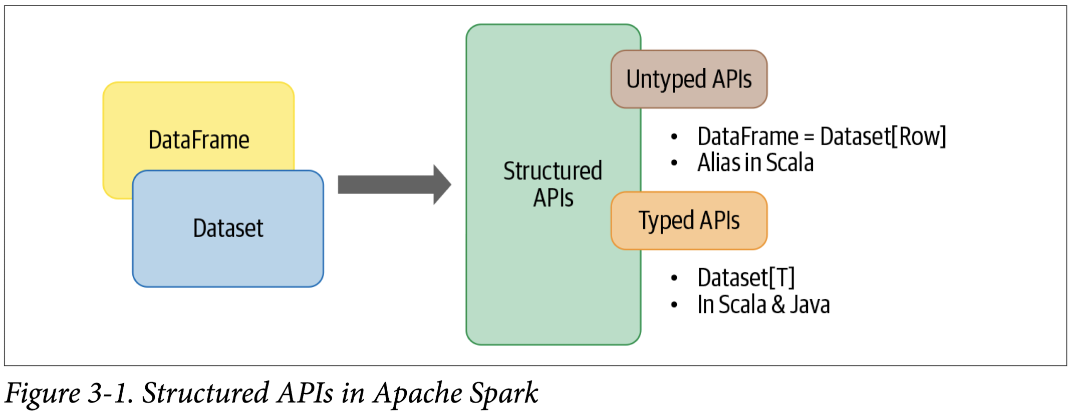
Conceptually, you can think of a DataFrame in Scala as an alias for a collection of generic objects, Dataset[Row], where a Row is a generic untyped JVM object that may hold different types of fields. A Dataset, by contrast, is a collection of strongly typed JVM objects in Scala or a class in Java. Or, as the Dataset documentation puts it, a Dataset is:
a strongly typed collection of domain-specific objects that can be transformed in parallel using functional or relational operations. Each Dataset [in Scala] also has an untyped view called a DataFrame, which is a Dataset of
Row.
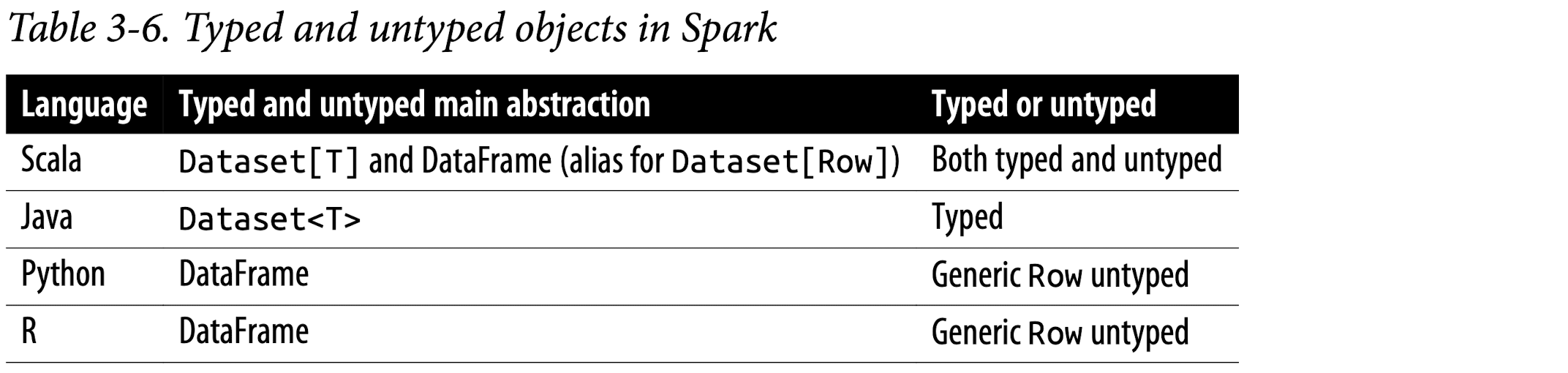
Typed Objects, Untyped Objects, and Generic Rows
In Spark’s supported languages, Datasets make sense only in Java and Scala, whereas in Python and R only DataFrames make sense. This is because Python and R are not compile-time type-safe; types are dynamically inferred or assigned during execution, not during compile time. The reverse is true in Scala and Java: types are bound to variables and objects at compile time. In Scala, however, a DataFrame is just an alias for untyped Dataset[Row]. Table 3-6 distills it in a nutshell.
SKIP for now since Dataset API only supports JAVA and Scala.
DataFrames Versus Datasets
By now you may be wondering why and when you should use DataFrames or Data‐ sets. In many cases either will do, depending on the languages you are working in, but there are some situations where one is preferable to the other. Here are a few examples:
- If you want to tell Spark what to do, not how to do it, use DataFrames or Datasets.
- If you want rich semantics, high-level abstractions, and DSL operators, use DataFrames or Datasets.
- If you want strict compile-time type safety and don’t mind creating multiple case classes for a specific
Dataset[T], use Datasets. - If your processing demands high-level expressions, filters, maps, aggregations, computing averages or sums, SQL queries, columnar access, or use of relational operators on semi-structured data, use DataFrames or Datasets.
- If your processing dictates relational transformations similar to SQL-like queries, use DataFrames.
- If you want to take advantage of and benefit from Tungsten’s efficient serialization with Encoders, use Datasets.
- If you want unification, code optimization, and simplification of APIs across Spark components, use DataFrames.
- If you are an R user, use DataFrames.
- If you are a Python user, use DataFrames and drop down to RDDs if you need more control.
- If you want space and speed efficiency, use DataFrames.
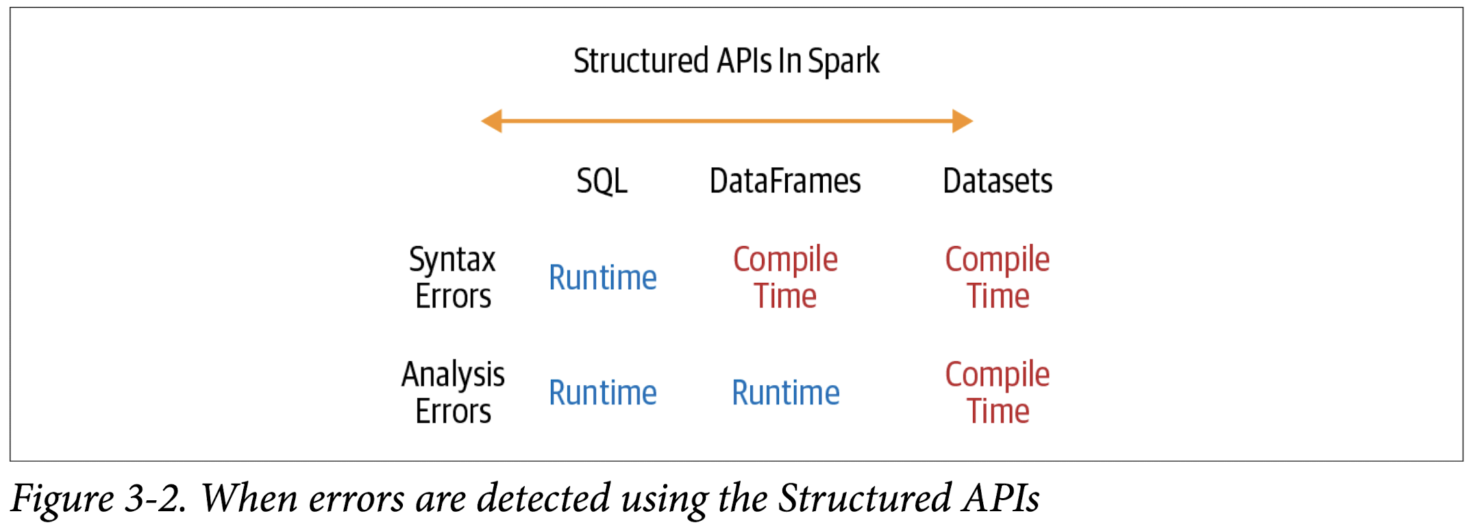
- If you want errors caught during compilation rather than at runtime, choose the
appropriate API as depicted in Figure 3-2.
When to User RDDs
You may ask: Are RDDs being relegated to second-class citizens? Are they being deprecated? The answer is a resounding no! The RDD API will continue to be supported, although all future development work in Spark 2.x and Spark 3.0 will continue to have a DataFrame interface and semantics rather than using RDDs.
There are some scenarios where you’ll want to consider using RDDs, such as when you:
- Are using a third-party package that’s written using RDDs
- Can forgo the code optimization, efficient space utilization, and performance benefits available with DataFrames and Datasets
- Want to precisely instruct Spark how to do a query
What’s more, you can seamlessly move between DataFrames or Datasets and RDDs at will using a simple API method call, df.rdd. (Note, however, that this does have a cost and should be avoided unless necessary.) After all, DataFrames and Datasets are built on top of RDDs, and they get decomposed to compact RDD code during whole-stage code generation.
Spark SQL and the Underlying Engine
At a programmatic level, Spark SQL allows developers to issue ANSI SQL:2003–compatible queries on structured data with a schema. Since its introduction in Spark 1.3, Spark SQL has evolved into a substantial engine upon which many high-level structured functionalities have been built. Apart from allowing you to issue SQL-like queries on your data, the Spark SQL engine:
- Unifies Spark components and permits abstraction to DataFrames/Datasets in Java, Scala, Python, and R, which simplifies working with structured data sets.
- Connects to the Apache Hive metastore and tables.
- Reads and writes structured data with a specific schema from structured file formats (JSON, CSV, Text, Avro, Parquet, ORC, etc.) and converts data into temporary tables.
- Offers an interactive Spark SQL shell for quick data exploration.
- Provides a bridge to (and from) external tools via standard database JDBC/ ODBC connectors.
- Generates optimized query plans and compact code for the JVM, for final execution.
Figure 3-3 shows the components that Spark SQL interacts with to achieve all of this.
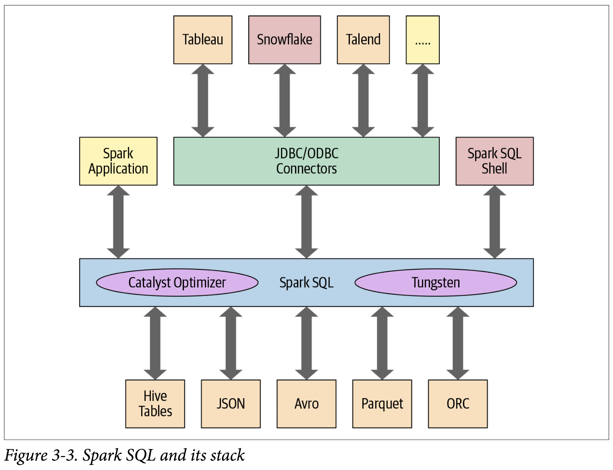
At the core of the Spark SQL engine are the Catalyst optimizer and Project Tungsten. Together, these support the high-level DataFrame and Dataset APIs and SQL queries.
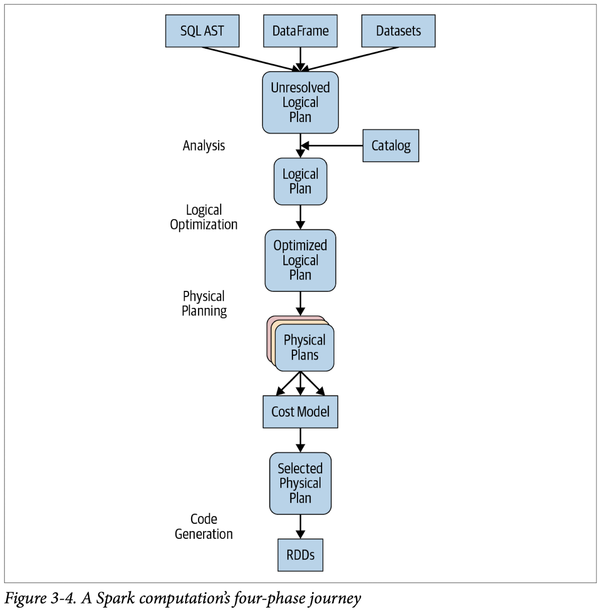
The Catalyst Optimizer
The Catalyst optimizer takes a computational query and converts it into an execution plan. It goes through four transformational phases, as shown in Figure 3-4:
- Analysis
- Logical optimization
- Physical planning
- Code generation
For example, consider one of the queries from our M&Ms example in Chapter 2. Both of the following sample code blocks will go through the same process, eventually ending up with a similar query plan and identical bytecode for execution. That is, regardless of the language you use, your computation undergoes the same journey and the resulting bytecode is likely the same:
1 | # In Python |
1 | -- In SQL |
To see the different stages the Python code goes through, you can use the count_mnm_df.explain(True) method on the DataFrame. Or, to get a look at the different logical and physical plans, in Scala you can call df.queryExecution.logical or df.queryExecution.optimizedPlan. (In Chapter 7, we will discuss more about tuning and debugging Spark and how to read query plans.) This gives us the follow‐ ing output:
Under directory chapter2/py/src:
1 | pyspark |
1 | import pyspark.sql.functions as F |
1 | +-----+------+-----+ |
1 | == Parsed Logical Plan == |
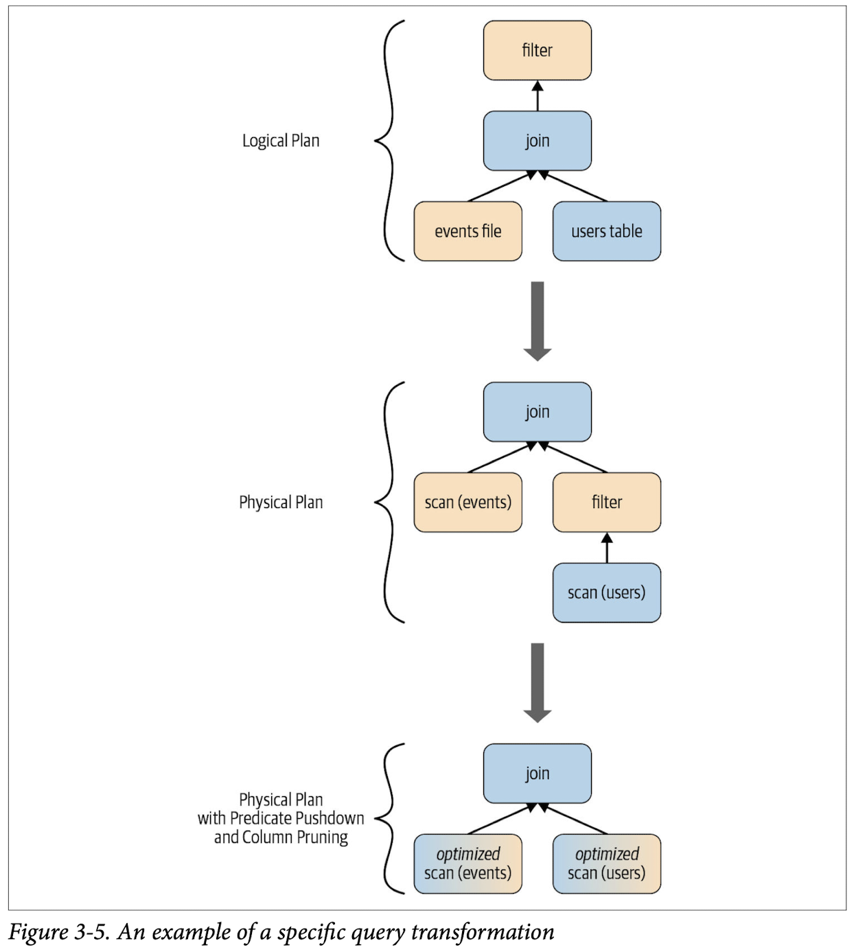
After going through an initial analysis phase, the query plan is transformed and rear-ranged by the Catalyst optimizer as shown in Figure 3-5.
Let’s go through each of the four query optimization phases..
Phase 1: Analysis
The Spark SQL engine begins by generating an abstract syntax tree (AST) for the SQL or DataFrame query. In this initial phase, any columns or table names will be resolved by consulting an internal Catalog, a programmatic interface to Spark SQL that holds a list of names of columns, data types, functions, tables, databases, etc. Once they’ve all been successfully resolved, the query proceeds to the next phase.
Phase 2: Logical optimization
As Figure 3-4 shows, this phase comprises two internal stages. Applying a standard- rule based optimization approach, the Catalyst optimizer will first construct a set of multiple plans and then, using its cost-based optimizer (CBO), assign costs to each plan. These plans are laid out as operator trees (like in Figure 3-5); they may include, for example, the process of constant folding, predicate pushdown, projection prun‐ ing, Boolean expression simplification, etc. This logical plan is the input into the physical plan.
Phase 3: Physical planning
In this phase, Spark SQL generates an optimal physical plan for the selected logical plan, using physical operators that match those available in the Spark execution engine.
Phase 4: Code generation
The final phase of query optimization involves generating efficient Java bytecode to run on each machine. Because Spark SQL can operate on data sets loaded in memory, Spark can use state-of-the-art compiler technology for code generation to speed up execution. In other words, it acts as a compiler. Project Tungsten, which facilitates whole-stage code generation, plays a role here.
Just what is whole-stage code generation? It’s a physical query optimization phase that collapses the whole query into a single function, getting rid of virtual function calls and employing CPU registers for intermediate data. The second-generation Tungsten engine, introduced in Spark 2.0, uses this approach to generate compact RDD code for final execution. This streamlined strategy significantly improves CPU efficiency and performance.
Summary
In this chapter, we took a deep dive into Spark’s Structured APIs, beginning with a look at the history and merits of structure in Spark.
Through illustrative common data operations and code examples, we demonstrated that the high-level DataFrame and Dataset APIs are far more expressive and intuitive than the low-level RDD API. Designed to make processing of large data sets easier, the Structured APIs provide domain-specific operators for common data operations, increasing the clarity and expressiveness of your code.
We explored when to use RDDs, DataFrames, and Datasets, depending on your use case scenarios.
And finally, we took a look under the hood to see how the Spark SQL engine’s main components—the Catalyst optimizer and Project Tungsten—support structured high- level APIs and DSL operators. As you saw, no matter which of the Spark-supported languages you use, a Spark query undergoes the same optimization journey, from log‐ ical and physical plan construction to final compact code generation.
The concepts and code examples in this chapter have laid the groundwork for the next two chapters, in which we will further illustrate the seamless interoperability between DataFrames, Datasets, and Spark SQL.
Spark SQL and DataFrames: Introduction to Built-in Data Sources
In particular, Spark SQL:
- Provides the engine upon which the high-level Structured APIs we explored in Chapter 3 are built.
- Can read and write data in a variety of structured formats (e.g., JSON, Hive tables, Parquet, Avro, ORC, CSV).
- Lets you query data using JDBC/ODBC connectors from external business intelligence (BI) data sources such as Tableau, Power BI, Talend, or from RDBMSs such as MySQL and PostgreSQL.
- Provides a programmatic interface to interact with structured data stored as tables or views in a database from a Spark application.
- Offers an interactive shell to issue SQL queries on your structured data.
- Supports ANSI SQL:2003-compliant commands and HiveQL.
Using Spark SQL in Spark Applications
The SparkSession provides a unified entry point for programming Spark with the Structured APIs. You can use a SparkSession to access Spark functionality: just import the class and create an instance in your code.
To issue any SQL query, use the sql() method on the SparkSession instance, spark, such as spark.sql("SELECT * FROM myTableName"). All spark.sql queries executed in this manner return a DataFrame on which you may perform further Spark operations if you desire.
Basic Query Examples
Spark SQL
Dataset: Airline On-Time Performance and Causes of Flight Delays
To use Spark SQL:
- Read dataset into a DataFrame.
- Register the DataFrame as a temporary view (more on temporary views shortly) so we can query it with SQL.
Normally, in a standalone Spark application, you will create a SparkSession instance manually, as shown in the following example. However, in a Spark shell (or Databricks notebook), the SparkSession is created for you and accessible via the appropriately named variable spark.
1 | from pyspark.sql import SparkSession |
Now that we have a temporary view, we can issue SQL queries using Spark SQL. These queries are no different from those you might issue against a SQL table in, say, a MySQL or PostgreSQL database. The point here is to show that Spark SQL offers an ANSI:2003–compliant SQL interface, and to demonstrate the interoperability between SQL and DataFrames.
The US flight delays data set has five columns:
- The date column contains a string like 02190925. When converted, this maps to 02-19 09:25 am.
- The delay column gives the delay in minutes between the scheduled and actual departure times. Early departures show negative numbers.
- The distance column gives the distance in miles from the origin airport to the destination airport.
- The origin column contains the origin IATA airport code.
- The destination column contains the destination IATA airport code.
With that in mind, let’s try some example queries against this data set. First, we’ll find all flights whose distance is greater than 1,000 miles:
1 | sqlquery = """ |
1 | +--------+------+-----------+ |
As the results show, all of the longest flights were between Honolulu (HNL) and New York (JFK). Next, we’ll find all flights between San Francisco (SFO) and Chicago (ORD) with at least a two-hour delay:
1 | sqlquery = """ |
1 | +-------+-----+------+-----------+ |
It seems there were many significantly delayed flights between these two cities, on different dates. (As an exercise, convert the date column into a readable format and find the days or months when these delays were most common. Were the delays related to winter months or holidays?)
Let’s try a more complicated query where we use the CASE clause in SQL. In the following example, we want to label all US flights, regardless of origin and destination, with an indication of the delays they experienced: Very Long Delays (> 6 hours), Long Delays (2–6 hours), etc. We’ll add these human-readable labels in a new column called Flight_Delays:
1 | # Spark SQL API |
1 | +-----+------+-----------+-------------+ |
1 | # Spark SQL API |
1 | +----------------+------+ |
As with the DataFrame and Dataset APIs, with the spark.sql interface you can conduct common data analysis operations like those we explored in the previous chapter. The computations undergo an identical journey in the Spark SQL engine (see “The Catalyst Optimizer” on page 77 in Chapter 3 for details), giving you the same results.
All three of the preceding SQL queries can be expressed with an equivalent DataFrame API query. For example, the first query can be expressed in the Python DataFrame API as:
1 | # DataFrame API |
Or
1 | # DataFrame API |
This produces the same results as the SQL query:
1 | +--------+------+-----------+ |
Try to perform the same query through DataFrame API.
1 | from pyspark.sql.functions import expr, asc, desc |
Or
1 | (df.select("delay", "origin", "destination", expr(case)) |
1 | +-----+------+-----------+-------------+ |
SQL Tables and Views
Tables hold data. Associated with each table in Spark is its relevant metadata, which is information about the table and its data: the schema, description, table name, database name, column names, partitions, physical location where the actual data resides, etc. All of this is stored in a central metastore.
Instead of having a separate metastore for Spark tables, Spark by default uses the Apache Hive metastore, located at /user/hive/warehouse, to persist all the metadata about your tables. However, you may change the default location by setting the Spark config variable spark.sql.warehouse.dir to another location, which can be set to a local or external distributed storage.
Managed Versus UnmanagedTables
Spark allows you to create two types of tables: managed and unmanaged.
- For a managed table, Spark manages both the metadata and the data in the file store. This could be a local filesystem, HDFS, or an object store such as Amazon S3 or Azure Blob.
- For an unmanaged table, Spark only manages the metadata, while you manage the data yourself in an external data source such as Cassandra.
With a managed table, because Spark manages everything, a SQL command such as DROP TABLE table_name deletes both the metadata and the data. With an unmanaged table, the same command will delete only the metadata, not the actual data. We will look at some examples of how to create managed and unmanaged tables in the next section.
Creating SQL Databases and Tables
Tables reside within a database. By default, Spark creates tables under the default database. To create your own database name, you can issue a SQL command from your Spark application or notebook. Using the US flight delays data set, let’s create both a managed and an unmanaged table. To begin, we’ll create a database called learn_spark_db and tell Spark we want to use that database:
1 | from os.path import abspath |
1 | # Path to data set |
1 | # create database and use database |
From this point, any commands we issue in our application to create tables will result in the tables being created in this database and residing under the database name learn_spark_db.
Creating a managed table
To create a managed table within the database learn_spark_db, you can issue a SQL query like the following:
1 | sqlQuery = """ |
You can do the same thing using the DataFrame API like this:
1 | # drop managed_us_delay_flights_tbl we create through Spark SQL API |
Both of these statements will create the managed table us_delay_flights_tbl in the learn_spark_db database.
Creating an unmanaged table
By contrast, you can create unmanaged tables from your own data sources—say, Parquet, CSV, or JSON files stored in a file store accessible to your Spark application.
To create an unmanaged table from a data source such as a CSV file, in SQL use:
1 | sqlQuery = f""" |
And within the DataFrame API use:
1 | # drop table we created in previous steps |
Creating Views
In addition to creating tables, Spark can create views on top of existing tables. Views can be global (visible across all SparkSessions on a given cluster) or session-scoped (visible only to a single SparkSession), and they are temporary: they disappear after your Spark application terminates.
Creating views has a similar syntax to creating tables within a database. Once you cre‐ ate a view, you can query it as you would a table. The difference between a view and a table is that views don’t actually hold the data; tables persist after your Spark applica‐ tion terminates, but views disappear.
You can create a view from an existing table using SQL. For example, if you wish to work on only the subset of the US flight delays data set with origin airports of New York (JFK) and San Francisco (SFO), the following queries will create global temporary and temporary views consisting of just that slice of the table:
1 | sqlQuery = """ |
Once you’ve created these views, you can issue queries against them just as you would against a table. Keep in mind that when accessing a global temporary view you must use the prefix global_temp.<view_name>, because Spark creates global temporary views in a global temporary database called global_temp. For example:
1 | # query global view from global_temp |
1 | +--------+-----+------+-----------+ |
By contrast, you can access the normal temporary view without the global_temp prefix:
1 | # query temporary view from current database |
1 | +--------+-----+------+-----------+ |
You can accomplish the same thing with the DataFrame API as follows:
1 | df_sfo = spark.sql("SELECT date, delay, origin, destination FROM us_delay_flights_tbl WHERE origin = 'SFO'") |
You can also query table from DataFrame API:
1 | # query global view from global_temp |
1 | # query temporary view from current database |
To show views:
1 | # List all views in global temp view database and current database |
Or:
1 | # List all views in global temp view database and current database |
To drop views:
1 | # drop views |
Or
1 | # drop views |
Temporary views versus global temporary views
The difference between temporary and global temporary views being subtle, it can be a source of mild confusion among developers new to Spark. A temporary view is tied to a single SparkSession within a Spark application. In contrast, a global temporary view is visible across multiple SparkSessions within a Spark application. Yes, you can create multiple SparkSessions within a single Spark application—this can be handy, for example, in cases where you want to access (and combine) data from two different SparkSessions that don’t share the same Hive metastore configurations.
Viewing the Metadata
As mentioned previously, Spark manages the metadata associated with each managed or unmanaged table. This is captured in the Catalog, a high-level abstraction in Spark SQL for storing metadata. The Catalog’s functionality was expanded in Spark 2.x with new public methods enabling you to examine the metadata associated with your databases, tables, and views. Spark 3.0 extends it to use external catalog (which we briefly discuss in Chapter 12).
For example, within a Spark application, after creating the SparkSession variable spark, you can access all the stored metadata through methods like these:
1 | spark.catalog.listDatabases() |
Caching SQL Tables
Although we will discuss table caching strategies in the next chapter, it’s worth mentioning here that, like DataFrames, you can cache and uncache SQL tables and views. In Spark 3.0, in addition to other options, you can specify a table as LAZY, meaning that it should only be cached when it is first used instead of immediately:
1 | -- In SQL |
Reading Tables into DataFrames
Often, data engineers build data pipelines as part of their regular data ingestion and ETL processes. They populate Spark SQL databases and tables with cleansed data for consumption by applications downstream.
Let’s assume you have an existing database, learn_spark_db, and table, us_delay_flights_tbl, ready for use. Instead of reading from an external JSON file, you can simply use SQL to query the table and assign the returned result to a DataFrame:
1 | pyspark |
1 | spark.catalog.listDatabases() |
The second database learn_spark_db was created by us in previous steps.
1 | spark.catalog.listTables('learn_spark_db') |
1 | # In Python |
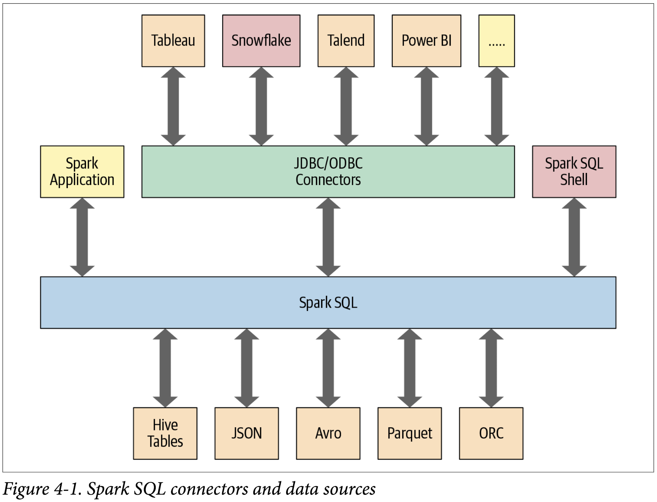
Data Sources for DataFrames and SQL Tables
As shown in Figure 4-1, Spark SQL provides an interface to a variety of data sources. It also provides a set of common methods for reading and writing data to and from these data sources using the Data Sources API.
In this section we will cover some of the built-in data sources, available file formats, and ways to load and write data, along with specific options pertaining to these data sources. But first, let’s take a closer look at two high-level Data Source API constructs that dictate the manner in which you interact with different data sources: DataFrameReader and DataFrameWriter.
DataFrameReader
DataFrameReader is the core construct for reading data from a data source into a DataFrame. It has a defined format and a recommended pattern for usage:
1 | DataFrameReader.format(args).option("key", "value").schema(args).load() |
This pattern of stringing methods together is common in Spark, and easy to read.
Note that you can only access a DataFrameReader through a SparkSession instance. That is, you cannot create an instance of DataFrameReader. To get an instance handle to it, use:
1 | # read static data |
1 | # read streaming data |
While read returns a handle to DataFrameReader to read into a DataFrame from a static data source, readStream returns an instance to read from a streaming source.
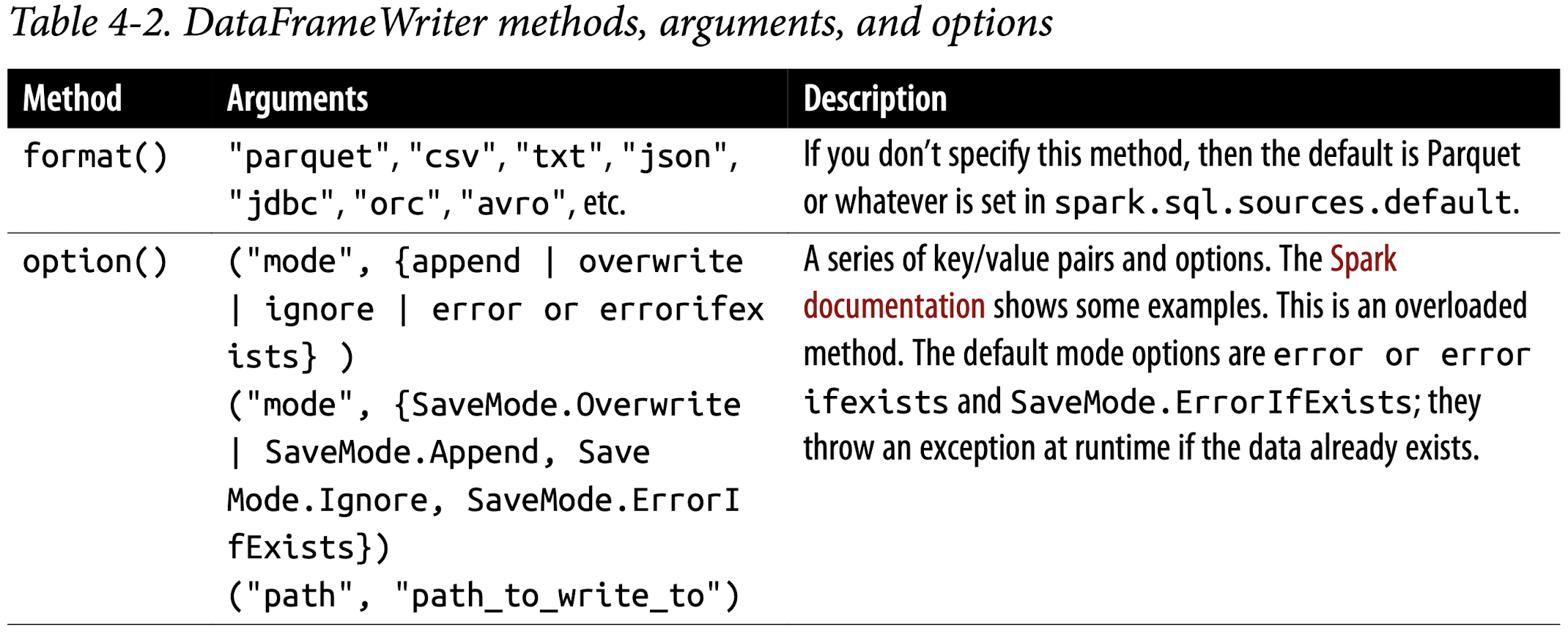
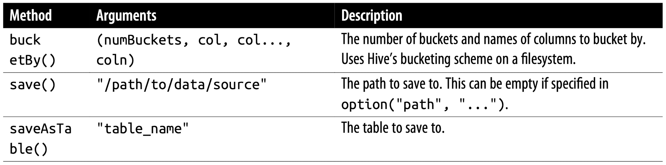
Arguments to each of the public methods to DataFrameReader take different values. Table 4-1 enumerates these, with a subset of the supported arguments.
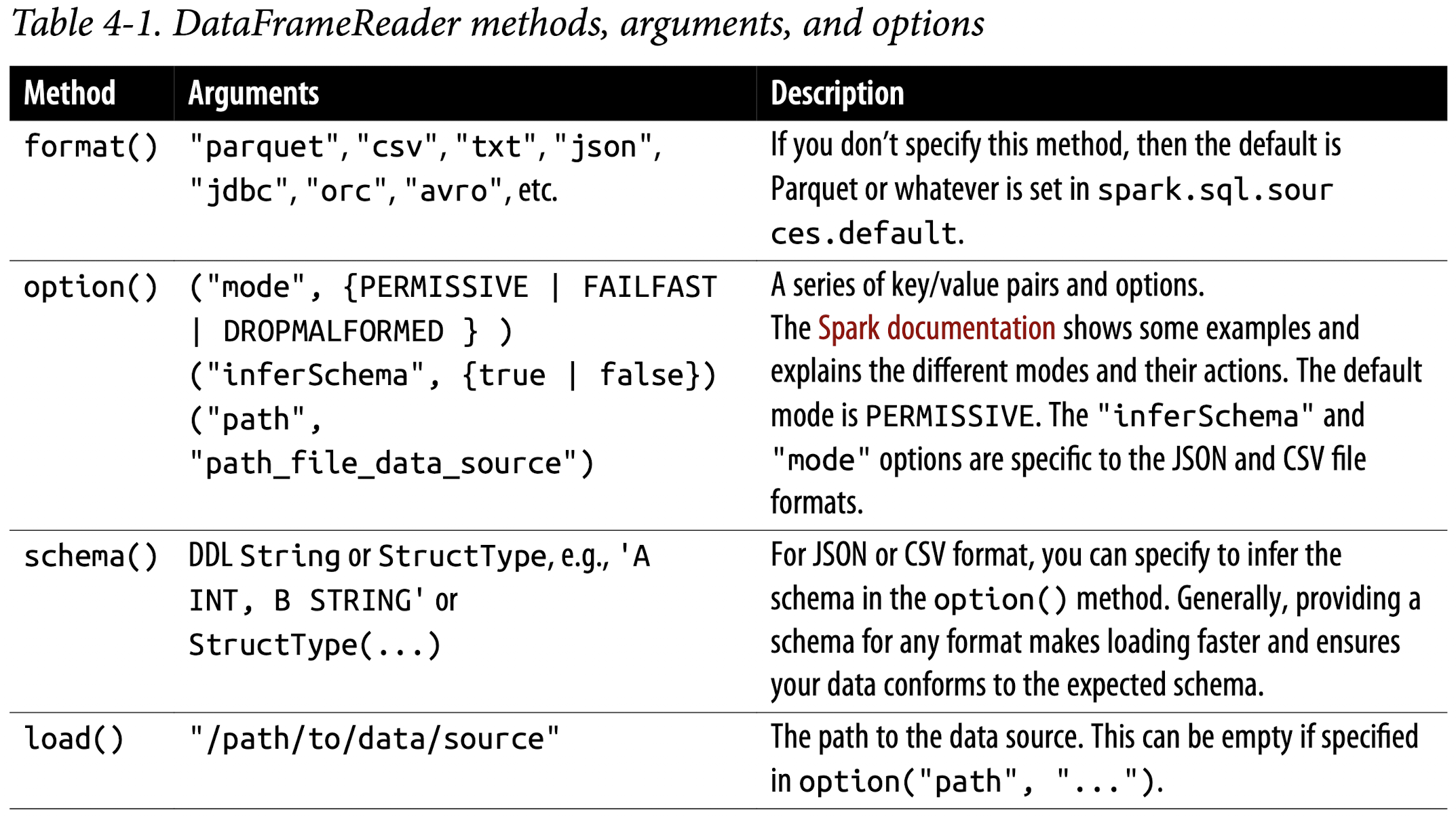
The documentation for Python, Scala, R, and Java offers suggestions and guidance.
In general, no schema is needed when reading from a static Parquet data source—the Parquet metadata usually contains the schema, so it’s inferred. However, for streaming data sources you will have to provide a schema.
Parquet is the default and preferred data source for Spark because it’s efficient, uses columnar storage, and employs a fast compression algorithm. You will see additional benefits later (such as columnar pushdown), when we cover the Catalyst optimizer in greater depth.
DataFrameWriter
DataFrameWriter does the reverse of its counterpart: it saves or writes data to a specified built-in data source. Unlike with DataFrameReader, you access its instance not from a SparkSession but from the DataFrame you wish to save. It has a few recommended usage patterns:
1 | DataFrameWriter.format(args) |
To get an instance handle, use:
1 | # write static data |
1 | # write streaming data |
Parqet
Parquet is the default data source in Spark. Supported and widely used by many big data processing frameworks and platforms, Parquet is an open source columnar file format that offers many I/O optimizations (such as compression, which saves storage space and allows for quick access to data columns).
Because of its efficiency and these optimizations, we recommend that after you have transformed and cleansed your data, you save your DataFrames in the Parquet format for downstream consumption. (Parquet is also the default table open format for Delta Lake, which we will cover in Chapter 9.)
Reading Parquet files into a DataFrame
Parquet files are stored in a directory structure that contains the data files, metadata, a number of compressed files, and some status files. Metadata in the footer contains the version of the file format, the schema, and column data such as the path, etc.
For example, a directory in a Parquet file might contain a set of files like this:
1 | _SUCCESS |
There may be a number of part-XXXX compressed files in a directory (the names shown here have been shortened to fit on the page).
To read Parquet files into a DataFrame, you simply specify the format and path:
1 | file = """databricks-datasets/learning-spark-v2/flights/summary-data/parquet/2010-summary.parquet/""" |
1 | +-----------------+-------------------+-----+ |
Unless you are reading from a streaming data source there’s no need to supply the schema, because Parquet saves it as part of its metadata.
Reading Parquet files into a Spark SQL table
As well as reading Parquet files into a Spark DataFrame, you can also create a Spark SQL unmanaged table or view directly using SQL:
1 | sqlQuery = """ |
1 | +-----------------+-------------------+-----+ |
Writing DataFrames to Parquet files
Writing or saving a DataFrame as a table or file is a common operation in Spark. To write a DataFrame you simply use the methods and arguments to the DataFrameWriter, supplying the location to save the Parquet files to. For example:
1 | # In Python |
Recall that Parquet is the default file format. If you don’t include the
format()method, the DataFrame will still be saved as a Parquet file.
This will create a set of compact and compressed Parquet files at the specified path. Since we used snappy as our compression choice here, we’ll have snappy compressed files. For brevity, this example generated only one file; normally, there may be a dozen or so files created:
1 | -rw-r--r-- 1 jules wheel 0 May 19 10:58 _SUCCESS |
Writing DataFrames to Spark SQL tables
Writing a DataFrame to a SQL table is as easy as writing to a file—just use saveAsTable() instead of save(). This will create a managed table called us_delay_flights_tbl:
1 | # In Python |
To sum up, Parquet is the preferred and default built-in data source file format in Spark, and it has been adopted by many other frameworks. We recommend that you use this format in your ETL and data ingestion processes.
JSON
JavaScript Object Notation (JSON) is also a popular data format. It came to prominence as an easy-to-read and easy-to-parse format compared to XML. It has two representational formats: single-line mode and multiline mode. Both modes are supported in Spark.
You can read JSON files in single-line or multi-line mode. In single-line mode, a file can be split into many parts and read in parallel. In multi-line mode, a file is loaded as a whole entity and cannot be split.
In single-line mode each line denotes a single JSON object, whereas in multiline mode the entire multiline object constitutes a single JSON object. To read in this mode, set multiLine to true in the option() method.
Reading JSON files into a DataFrame
You can read a JSON file into a DataFrame the same way you did with Parquet—just specify “json“ in the format() method:
1 | ➜ LearningSparkV2 git:(dev) ✗ ll databricks-datasets/learning-spark-v2/flights/summary-data/json |
1 | # read multiple JSON files |
1 | +-----------------+-------------------+-----+ |
Reading JSON files into a Spark SQL table
You can also create a SQL table from a JSON file just like you did with Parquet:
1 | sqlQuery = """ |
1 | +-----------------+-------------------+-----+ |
Writing DataFrames to JSON files
Saving a DataFrame as a JSON file is simple. Specify the appropriate DataFrameWriter methods and arguments, and supply the location to save the JSON files to:
1 | (df.write.format("json") |
This creates a directory at the specified path populated with a set of compact JSON files:
1 | -rw-r--r-- 1 jules wheel 0 May 16 14:44 _SUCCESS |
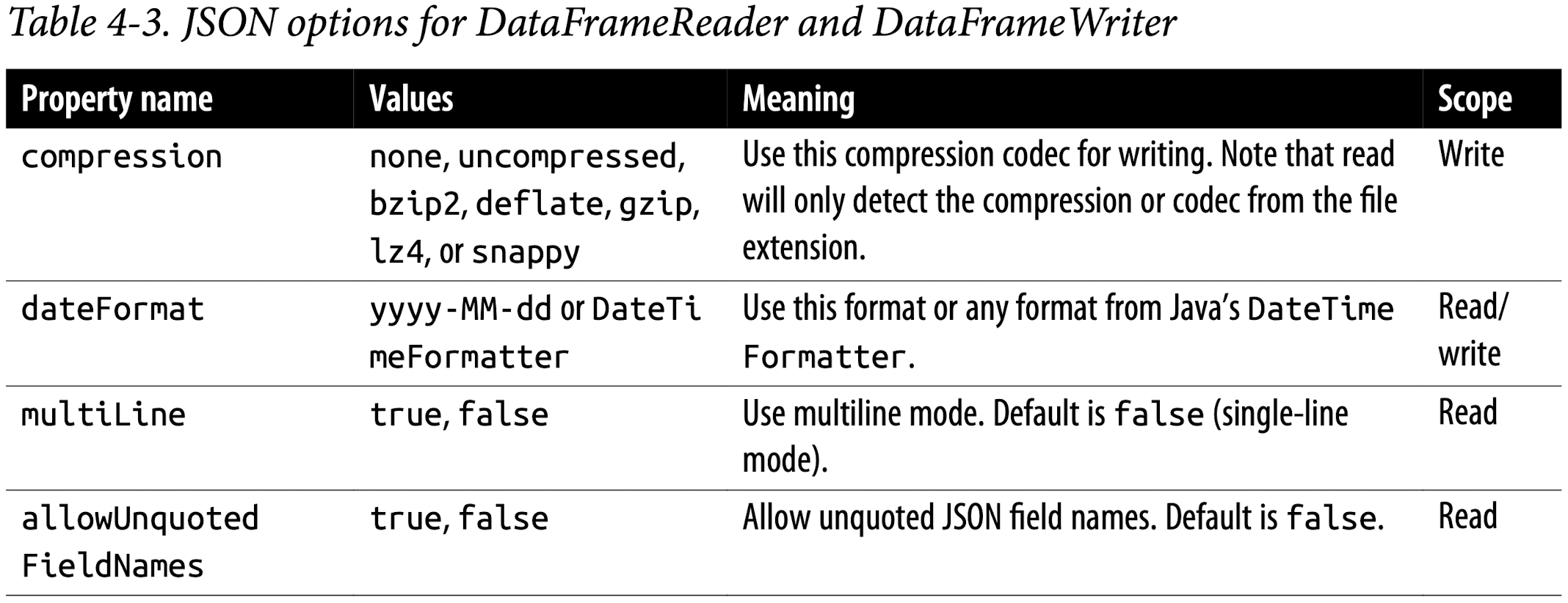
JSON data source options
Table 4-3 describes common JSON options for DataFrameReader and DataFrame Writer. For a comprehensive list, we refer you to the documentation.
CSV
As widely used as plain text files, this common text file format captures each datum or field delimited by a comma; each line with comma-separated fields represents a record. Even though a comma is the default separator, you may use other delimiters to separate fields in cases where commas are part of your data. Popular spreadsheets can generate CSV files, so it’s a popular format among data and business analysts.
Reading a CSV file into a DataFrame
As with the other built-in data sources, you can use the DataFrameReader methods and arguments to read a CSV file into a DataFrame:
1 | file = "databricks-datasets/learning-spark-v2/flights/summary-data/csv/*" |
1 | +-----------------+-------------------+-----+ |
Reading a CSV file into a Spark SQL table
Creating a SQL table from a CSV data source is no different from using Parquet or JSON:
1 | sqlQuery = """ |
1 | +-----------------+-------------------+-----+ |
Once you’ve created the table, you can read data into a DataFrame using SQL as before:
Writing DataFrames to CSV files
Saving a DataFrame as a CSV file is simple. Specify the appropriate DataFrameWriter methods and arguments, and supply the location to save the CSV files to:
1 | df.write.format("csv").mode("overwrite").save("/tmp/data/csv/df_csv") |
This generates a folder at the specified location, populated with a bunch of com‐
pressed and compact files:
1 | -rw-r--r-- 1 jules wheel 0 May 16 12:17 _SUCCESS |
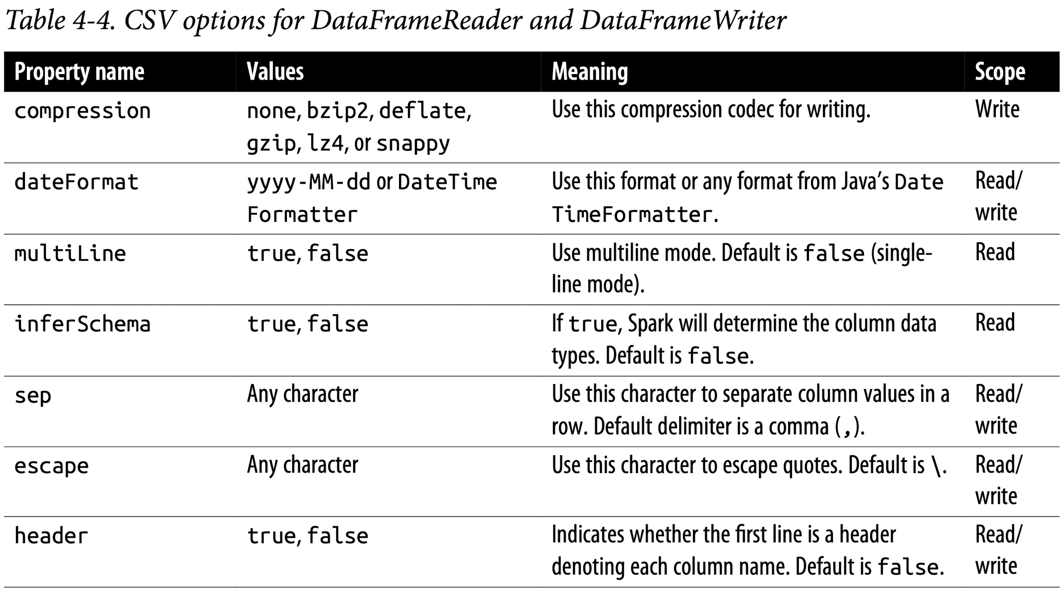
CSV data source options
Table 4-4 describes some of the common CSV options for DataFrameReader and DataFrameWriter. Because CSV files can be complex, many options are available; for a comprehensive list we refer you to the documentation.
Avro
Apache Avro Data Source Guide
Thespark-avromodule is external and not included inspark-submitorspark-shellby default.
Introduced in Spark 2.4 as a built-in data source, the Avro format is used, for example, by Apache Kafka for message serializing and deserializing. It offers many benefits, including direct mapping to JSON, speed and efficiency, and bindings available for many programming languages.
Reading an Avro file into a DataFrame
Reading an Avro file into a DataFrame using DataFrameReader is consistent in usage with the other data sources we have discussed in this section:
1 | ➜ LearningSparkV2 git:(dev) ✗ ll databricks-datasets/learning-spark-v2/flights/summary-data/avro/* |
1 | df = (spark.read.format("avro").load("databricks-datasets/learning-spark-v2/flights/summary-data/avro/*")) |
Reading an Avro file into a Spark SQL table
Again, creating SQL tables using an Avro data source is no different from using Par‐ quet, JSON, or CSV:
1 | -- In SQL |
Writing DataFrames to Avro files
Writing a DataFrame as an Avro file is simple. As usual, specify the appropriate DataFrameWriter methods and arguments, and supply the location to save the Avro files to:
1 | (df.write |
This generates a folder at the specified location, populated with a bunch of compressed and compact files:
1 | -rw-r--r-- 1 jules wheel 0 May 17 11:54 _SUCCESS |
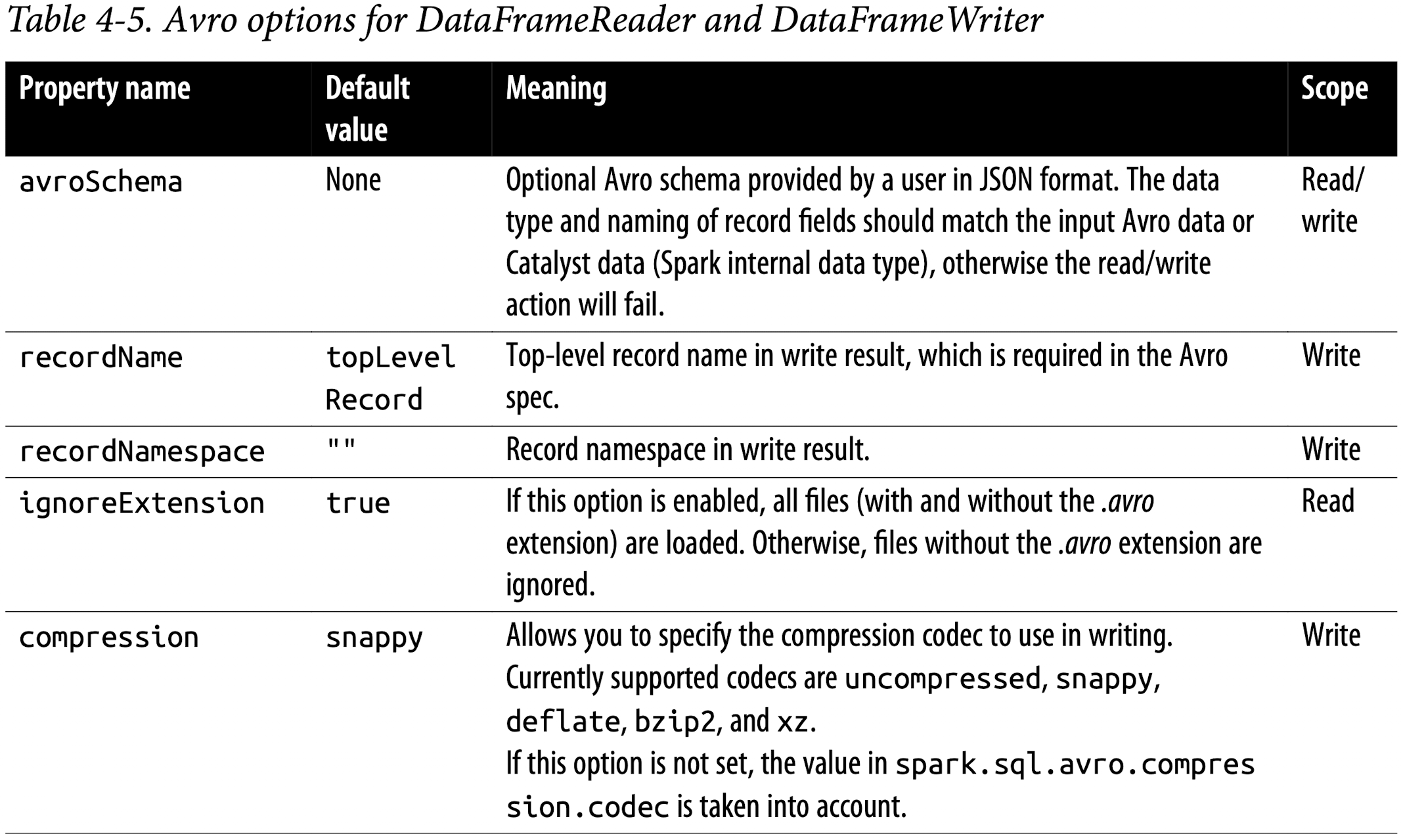
Avro data source options
Table 4-5 describes common options for DataFrameReader and DataFrameWriter. A comprehensive list of options is in the documentation.
ORC
As an additional optimized columnar file format, Spark 2.x supports a vectorized ORC reader. Two Spark configurations dictate which ORC implementation to use. When spark.sql.orc.impl is set to native and spark.sql.orc.enableVectorizedReader is set to true, Spark uses the vectorized ORC reader. A vectorized reader reads blocks of rows (often 1,024 per block) instead of one row at a time, streamlining operations and reducing CPU usage for intensive operations like scans, filters, aggre‐ gations, and joins.
For Hive ORC SerDe (serialization and deserialization) tables created with the SQL command USING HIVE OPTIONS (fileFormat ‘ORC’), the vectorized reader is used when the Spark configuration parameter spark.sql.hive.convertMetastoreOrc is set to true.
Reading an ORC file into a DataFrame
To read in a DataFrame using the ORC vectorized reader, you can just use the normal DataFrameReader methods and options:
1 | # In Python |
1 | +-----------------+-------------------+-----+ |
Reading an ORC file into a Spark SQL table
There is no difference from Parquet, JSON, CSV, or Avro when creating a SQL view using an ORC data source:
1 | sqlQuery = """ |
1 | +-----------------+-------------------+-----+ |
Writing DataFrames to ORC files
Writing back a transformed DataFrame after reading is equally simple using the DataFrameWriter methods:
1 | (df.write.format("orc") |
The result will be a folder at the specified location containing some compressed ORC files:
1 | -rw-r--r-- 1 jules wheel 0 May 16 17:23 _SUCCESS |
Images
In Spark 2.4 the community introduced a new data source, image files, to support deep learning and machine learning frameworks such as TensorFlow and PyTorch. For computer vision–based machine learning applications, loading and processing image data sets is important.
Reading an image file into a DataFrame
As with all of the previous file formats, you can use the DataFrameReader methods and options to read in an image file as shown here:
1 | from pyspark.ml import image |
1 | from pyspark.ml import image |
1 | root |
1 | images_df.select("image.height", "image.width", "image.nChannels", "image.mode", "label").show(5, truncate=False) |
1 | +------+-----+---------+----+-----+ |
Binary Files
Spark 3.0 adds support for binary files as a data source. The DataFrameReader converts each binary file into a single DataFrame row (record) that contains the raw content and metadata of the file. The binary file data source produces a DataFrame with the following columns:
- path: StringType
- modificationTime: TimestampType
- length: LongType
- content: BinaryType
Reading a binary file into a DataFrame
To read binary files, specify the data source format as a binaryFile. You can load files with paths matching a given global pattern while preserving the behavior of partition discovery with the data source option pathGlobFilter. For example, the following code reads all JPG files from the input directory with any partitioned directories:
1 | path = "databricks-datasets/learning-spark-v2/cctvVideos/train_images/" |
1 | +--------------------+--------------------+------+--------------------+-----+ |
To ignore partitioning data discovery in a directory, you can set recursiveFileLookup to “true“:
1 | path = "databricks-datasets/learning-spark-v2/cctvVideos/train_images/" |
1 | +--------------------+--------------------+------+--------------------+ |
Note that the label column is absent when the recursiveFileLookup option is set to “true“.
Currently, the binary file data source does not support writing a DataFrame back to the original file format.
Summary
To recap, this chapter explored the interoperability between the DataFrame API and Spark SQL. In particular, you got a flavor of how to use Spark SQL to:
- Create managed and unmanaged tables using Spark SQL and the DataFrame API.
- Read from and write to various built-in data sources and file formats.
- Employ the
spark.sqlprogrammatic interface to issue SQL queries on structured data stored as Spark SQL tables or views. - Peruse the Spark Catalog to inspect metadata associated with tables and views.
- Use the
DataFrameWriterandDataFrameReaderAPIs.
Spark SQL and DataFrames: Interacting with External Data Sources
In this chapter, we will focus on how Spark SQL interfaces with external components. Specifically, we discuss how Spark SQL allows you to:
- Use user-defined functions for both Apache Hive and Apache Spark.
- Connect with external data sources such as JDBC and SQL databases, PostgreSQL, MySQL, Tableau, Azure Cosmos DB, and MS SQL Server.
- Work with simple and complex types, higher-order functions, and common relational operators.
We’ll also look at some different options for querying Spark using Spark SQL, such as the Spark SQL shell, Beeline, and Tableau.
Spark SQL and Apache Hive
Spark SQL is a foundational component of Apache Spark that integrates relational processing with Spark’s functional programming API. Its genesis was in previous work on Shark. Shark was originally built on the Hive codebase on top of Apache Spark and became one of the first interactive SQL query engines on Hadoop systems. It demonstrated that it was possible to have the best of both worlds; as fast as an enterprise data warehouse, and scaling as well as Hive/MapReduce.
Spark SQL lets Spark programmers leverage the benefits of faster performance and relational programming (e.g., declarative queries and optimized storage), as well as call complex analytics libraries (e.g., machine learning). As discussed in the previous chapter, as of Apache Spark 2.x, the SparkSession provides a single unified entry point to manipulate data in Spark.
User-Defined Functions
While Apache Spark has a plethora of built-in functions, the flexibility of Spark allows for data engineers and data scientists to define their own functions too. These are known as user-defined functions (UDFs).
Spark SQL UDFs
The benefit of creating your own PySpark or Scala UDFs is that you (and others) will be able to make use of them within Spark SQL itself. For example, a data scientist can wrap an ML model within a UDF so that a data analyst can query its predictions in Spark SQL without necessarily understanding the internals of the model.
Here’s a simplified example of creating a Spark SQL UDF. Note that UDFs operate per session and they will not be persisted in the underlying metastore:
1 | # In Python |
1 | +---+--------+ |
Evaluation order and null checking in Spark SQL
Spark SQL (this includes SQL, the DataFrame API, and the Dataset API) does not guarantee the order of evaluation of subexpressions. For example, the following query does not guarantee that the s is NOT NULL clause is executed prior to the strlen(s) > 1 clause:
1 | spark.sql("SELECT s FROM test1 WHERE s IS NOT NULL AND strlen(s) > 1") |
Therefore, to perform proper null checking, it is recommended that you do the
following:
- Make the UDF itself
null-aware and donullchecking inside the UDF. - Use IF or
CASE WHENexpressions to do thenullcheck and invoke the UDF in a conditional branch.
Speeding up and distributing PySpark UDFs with Pandas UDFs
One of the previous prevailing issues with using PySpark UDFs was that they had slower performance than Scala UDFs. This was because the PySpark UDFs required data movement between the JVM and Python, which was quite expensive. To resolve this problem, Pandas UDFs (also known as vectorized UDFs) were introduced as part of Apache Spark 2.3. A Pandas UDF uses Apache Arrow to transfer data and Pandas to work with the data. You define a Pandas UDF using the keyword pandas_udf as the decorator, or to wrap the function itself. Once the data is in Apache Arrow format, there is no longer the need to serialize/pickle the data as it is already in a format consumable by the Python process. Instead of operating on individual inputs row by row, you are operating on a Pandas Series or DataFrame (i.e., vectorized execution).
From Apache Spark 3.0 with Python 3.6 and above, Pandas UDFs were split into two API categories: Pandas UDFs and Pandas Function APIs.
Pandas UDFs
With Apache Spark 3.0, Pandas UDFs infer the Pandas UDF type from Python type hints in Pandas UDFs such as pandas.Series, pandas.DataFrame, Tuple, and Iterator. Previously you needed to manually define and specify each Pandas UDF type. Currently, the supported cases of Python type hints in Pandas UDFs are Series to Series, Iterator of Series to Iterator of Series, Iterator of Multiple Series to Iterator of Series, and Series to Scalar (a single value).
Pandas Function APIs
Pandas Function APIs allow you to directly apply a local Python function to a PySpark DataFrame where both the input and output are Pandas instances. For Spark 3.0, the supported Pandas Function APIs are grouped map, map, co- grouped map.
The following is an example of a scalar Pandas UDF for Spark 3.0:
1 | # In Python |
The preceding code snippet declares a function called cubed() that performs a cubed operation. This is a regular Pandas function with the additional cubed_udf = pandas_udf() call to create our Pandas UDF.
Let’s start with a simple Pandas Series (as defined for x) and then apply the local func‐ tion cubed() for the cubed calculation:
1 | # Create a Pandas Series |
1 | 0 1 |
Now let’s switch to a Spark DataFrame. We can execute this function as a Spark vec‐ torized UDF as follows:
1 | # Create a Spark DataFrame, 'spark' is an existing SparkSession |
1 | +---+---------+ |
Notice the column name is cubed although we called cubed_udf.
For SQL:
1 | df.createOrReplaceTempView("_df") |
1 | +---+-------------+ |
As opposed to a local function, using a vectorized UDF will result in the execution of Spark jobs; the previous local function is a Pandas function executed only on the Spark driver. This becomes more apparent when viewing the Spark UI for one of the stages of this pandas_udf function (Figure 5-1).
For a deeper dive into Pandas UDFs, refer to pandas user-defined functions documentation.
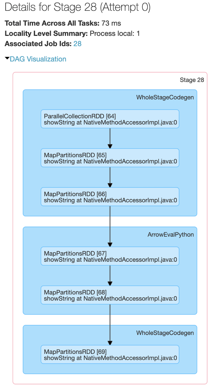
Figure 5-1. Spark UI stages for executing a Pandas UDF on a Spark DataFrame
Like many Spark jobs, the job starts with parallelize() to send local data (Arrow binary batches) to executors and calls mapPartitions() to convert the Arrow binary batches to Spark’s internal data format, which can be distributed to the Spark workers. There are a number of WholeStageCodegen steps, which represent a fundamental step up in performance (thanks to Project Tungsten’s whole-stage code generation, which significantly improves CPU efficiency and performance). But it is the ArrowEvalPython step that identifies that (in this case) a Pandas UDF is being executed.
Querying with the Spark SQL Shell, Beeline, and Tableau
There are various mechanisms to query Apache Spark, including the Spark SQL shell, the Beeline CLI utility, and reporting tools like Tableau and Power BI.
In this section, we include instructions for Tableau; for Power BI, please refer to the documentation.
Using the Spark SQL Shell
A convenient tool for executing Spark SQL queries is the spark-sql CLI. While this utility communicates with the Hive metastore service in local mode, it does not talk to the Thrift JDBC/ODBC server (a.k.a. Spark Thrift Server or STS). The STS allows JDBC/ODBC clients to execute SQL queries over JDBC and ODBC protocols on Apache Spark.
To start the Spark SQL CLI, execute the following command in the $SPARK_HOME folder:
1 | ./bin/spark-sql |
Or
1 | $SPARK_HOME/bin/spark-sql |
Once you’ve started the shell, you can use it to interactively perform Spark SQL queries. Let’s take a look at a few examples.
Create a table
To create a new permanent Spark SQL table, execute the following statement:
1 | -- we created learn_spark_db in previous chapters |
Your output should be similar to this, noting the creation of the Spark SQL table
people as well as its file location (/user/hive/warehouse/people):
Insert data into the table
You can insert data into a Spark SQL table by executing a statement similar to:
1 | INSERT INTO people SELECT name, age FROM ... |
As you’re not dependent on loading data from a preexisting table or file, you can insert data into the table using INSERT...VALUES statements. These three statements insert three individuals (their names and ages, if known) into the people table:
1 | spark-sql> INSERT INTO people VALUES ("Michael", NULL); |
Running a Spark SQL query
Now that you have data in your table, you can run Spark SQL queries against it. Let’s start by viewing what tables exist in our metastore:
1 | spark-sql> SHOW TABLES; |
Next, let’s find out how many people in our table are younger than 20 years of age:
1 | spark-sql> SELECT * FROM people WHERE age < 20; |
As well, let’s see who the individuals are who did not specify their age:
1 | spark-sql> SELECT name FROM people WHERE age IS NULL; |
Working with Beeline
If you’ve worked with Apache Hive you may be familiar with the command-line tool Beeline, a common utility for running HiveQL queries against HiveServer2. Beeline is a JDBC client based on the SQLLine CLI. You can use this same utility to execute Spark SQL queries against the Spark Thrift server. Note that the currently implemented Thrift JDBC/ODBC server corresponds to HiveServer2 in Hive 1.2.1. You can test the JDBC server with the following Beeline script that comes with either Spark or Hive 1.2.1.
Start the Thrift server
To start the Spark Thrift JDBC/ODBC server, execute the following command from the $SPARK_HOME folder:
1 | ./sbin/start-thriftserver.sh |
Or
1 | $SPARK_HOME/sbin/start-thriftserver.sh |
If you have not already started your Spark driver and worker, execute the following command prior to start-thriftserver.sh:
1 | ./sbin/start-all.sh |
Or
1 | $SPARK_HOME/sbin/start-all.sh |
Connect to the Thrift server via Beeline
To test the Thrift JDBC/ODBC server using Beeline, execute the following command:
1 | ./bin/beeline |
Or
1 | $SPARK_HOME/bin/beeline |
Then configure Beeline to connect to the local Thrift server:
1 | !connect jdbc:hive2://localhost:10000 |
By default, Beeline is in non-secure mode. Thus, the username is your login (e.g., user@learningspark.org) and the password is blank.
For example:
1 | beeline> !connect jdbc:hive2://localhost:10000 |
Execute a Spark SQL query with Beeline
From here, you can run a Spark SQL query similar to how you would run a Hive query with Beeline. Here are a few sample queries and their output:
1 | 0: jdbc:hive2://localhost:10000> USE learn_spark_db; |
1 | +-----------------+------------+--------------+ |
1 | 0: jdbc:hive2://localhost:10000> SELECT * FROM people; |
1 | +-----------+-------+ |
Stop the Thrift server
Once you’re done, you can stop the Thrift server with the following command:
1 | ./sbin/stop-thriftserver.sh |
Or
1 | $SPARK_HOME/sbin/stop-thriftserver.sh |
Working with Tableau
Similar to running queries through Beeline or the Spark SQL CLI, you can connect your favorite BI tool to Spark SQL via the Thrift JDBC/ODBC server. In this section, we will show you how to connect Tableau Desktop (version 2019.2) to your local Apache Spark instance.
You will need to have the Tableau’s Spark ODBC driver version 1.2.0 or above already installed. If you have installed (or upgraded to) Tableau 2018.1 or greater, this driver should already be preinstalled.
Start the Thrift server
To start the Spark Thrift JDBC/ODBC server, execute the following command from the $SPARK_HOME folder:
1 | ./sbin/start-thriftserver.sh |
Or
1 | $SPARK_HOME/sbin/start-thriftserver.sh |
If you have not already started your Spark driver and worker, execute the following command prior to start-thriftserver.sh:
1 | ./sbin/start-all.sh |
Or
1 | $SPARK_HOME/sbin/start-all.sh |
Skip for now since I don’t have Tableau license
External Data Sources
JDBC and SQL Databases
Spark SQL includes a data source API that can read data from other databases using
JDBC. It simplifies querying these data sources as it returns the results as a DataFrame, thus providing all of the benefits of Spark SQL (including performance and the ability to join with other data sources).
To get started, you will need to specify the JDBC driver for your JDBC data source and it will need to be on the Spark classpath. From the $SPARK_HOME folder, you’ll issue a command like the following:
1 | ./bin/spark-shell --driver-class-path $database.jar --jars $database.jar |
Using the data source API, the tables from the remote database can be loaded as a DataFrame or Spark SQL temporary view. Users can specify the JDBC connection properties in the data source options. Table 5-1 contains some of the more common connection properties (case-insensitive) that Spark supports.
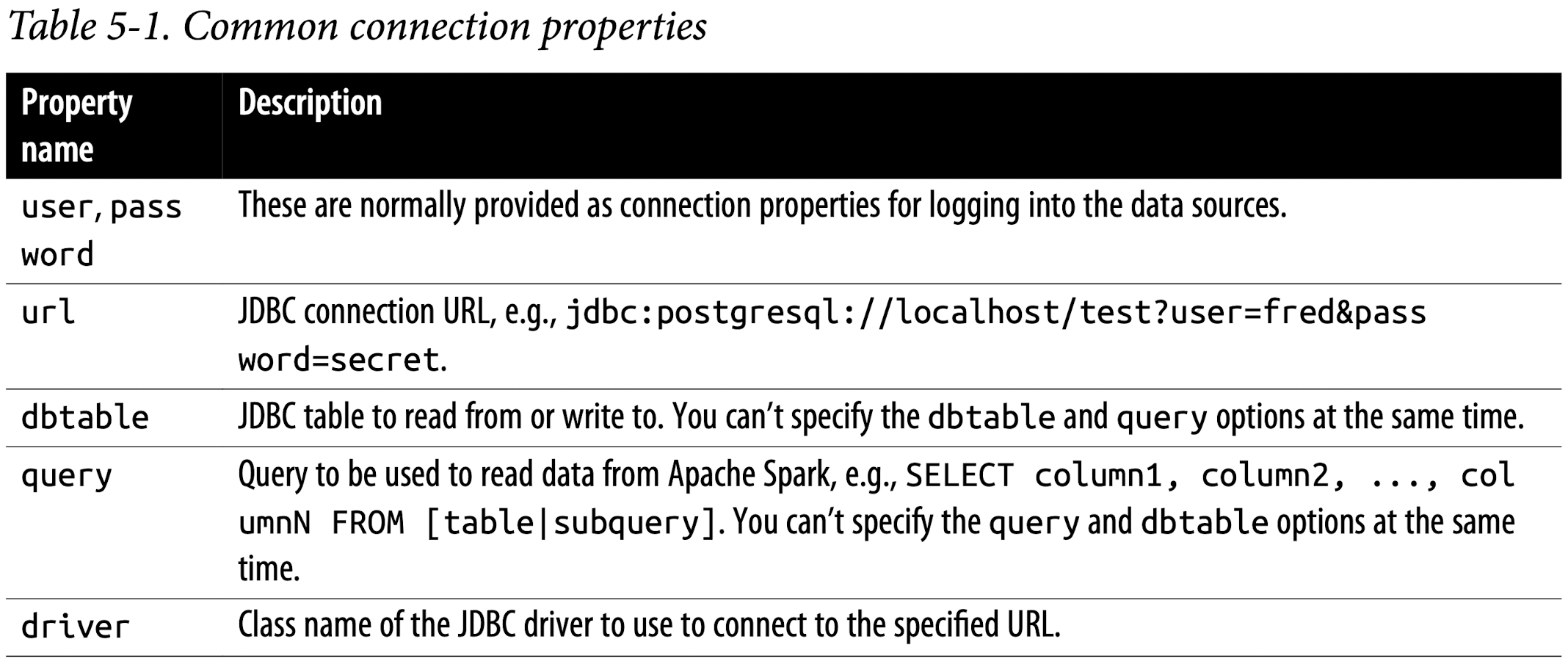
For the full list of connection properties, see the Spark SQL documentation.
Example: PySpark & MySQL
Download JDBC Connector
For MacOS, download and unzip MySQL JDBC connector -
Platform Independenton MySQL.
After unzip the MySQL JDBC file, you will get a connector directory.
Inside the directory, you can see there is a .jar file
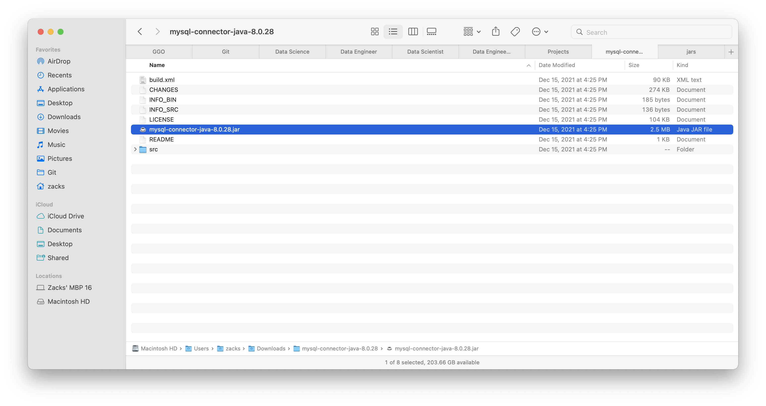
Save JDBC Connector inside Spark root directory
Make a directory named jdbc under your Spark root directoy:
1 | ➜ spark-3.2.1-bin-hadoop3.2 mkdir jdbc |
Move the whole MYSQL JDBC directory(e.g., the connector dir was in my Downloads dir) to jdbc:
1 | ➜ spark-3.2.1-bin-hadoop3.2 mv ~/Downloads/mysql-connector-java-8.0.28 jdbc |
Check:
Notice MySQL JDBC connector .jar file’s path is jdbc/mysql-connector-java-8.0.28/mysql-connector-java-8.0.28.jar
1 | ➜ spark-3.2.1-bin-hadoop3.2 ll jdbc/mysql-connector-java-8.0.28 |
Specify JDBC Connector for Spark classpath
Include applicable JDBC driver when you submit the application or start shell:
1 | bin/pyspark --driver-class-path jdbc/mysql-connector-java-8.0.28/mysql-connector-java-8.0.28.jar --jars jdbc/mysql-connector-java-8.0.28/mysql-connector-java-8.0.28.jar |
Test: PySpark
1 | # Loading data from a JDBC source using load |
1 | jdbcDF.show() |
The importance of partitioning
When transferring large amounts of data between Spark SQL and a JDBC external source, it is important to partition your data source. All of your data is going through one driver connection, which can saturate and significantly slow down the performance of your extraction, as well as potentially saturate the resources of your source system. While these JDBC properties are optional, for any large-scale operations it is highly recommended to use the properties shown in Table 5-2.
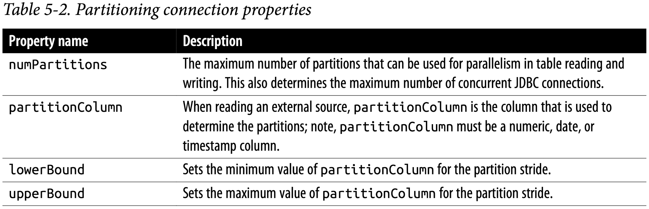
Let’s take a look at an example to help you understand how these properties work. Suppose we use the following settings:
numPartitions:10lowerBound:1000upperBound:10000
Then the stride is equal to 1,000, and 10 partitions will be created. This is the equivalent of executing these 10 queries (one for each partition):
SELECT *FROM table WHERE partitionColumn BETWEEN 1000 and 2000SELECT* FROM table WHERE partitionColumn BETWEEN 2000 and 3000...SELECT * FROM table WHERE partitionColumn BETWEEN 9000 and 10000
While not all-encompassing, the following are some hints to keep in mind when using these properties:
- A good starting point for
numPartitionsis to use a multiple of the number of Spark workers. For example, if you have four Spark worker nodes, then perhaps start with4or8partitions. But it is also important to note how well your source system can handle the read requests. For systems that have processing windows, you can maximize the number of concurrent requests to the source system; for systems lacking processing windows (e.g., an OLTP system continuously processing data), you should reduce the number of concurrent requests to prevent saturation of the source system. - Initially, calculate the
lowerBoundandupperBoundbased on the minimum and maximumpartitionColumnactual values. For example, if you choose{numPartitions:10, lowerBound: 1000, upperBound: 10000}, but all of the values are between 2000 and 4000, then only 2 of the 10 queries (one for each partition) will be doing all of the work. In this scenario, a better configuration would be {numPartitions:10, lowerBound: 2000, upperBound: 4000}. - Choose a
partitionColumnthat can be uniformly distributed to avoid data skew. For example, if the majority of yourpartitionColumnhas the value2500, with{numPartitions:10, lowerBound: 1000, upperBound: 10000}most of the work will be performed by the task requesting the values between2000and3000. Instead, choose a differentpartitionColumn, or if possible generate a new one (perhaps a hash of multiple columns) to more evenly distribute your partitions.
PostgreSQL
To connect to a PostgreSQL database, build or download the JDBC jar from Maven and add it to your classpath. Then start a Spark shell (spark-shell or pyspark), specifying that jar:
1 | bin/spark-shell --jars postgresql-42.2.6.jar |
The following examples show how to load from and save to a PostgreSQL database using the Spark SQL data source API and JDBC in PySpark:
1 | # Read Option 1: Loading data from a JDBC source using load method |
MySQL
To connect to a MySQL database, build or download the JDBC jar from Maven or MySQL (the latter is easier!) and add it to your classpath. Then start a Spark shell (spark-shell or pyspark), specifying that jar:
1 | bin/spark-shell --jars mysql-connector-java_8.0.16-bin.jar |
The following examples show how to load data from and save it to a MySQL database using the Spark SQL data source API and JDBC in PySpark:
1 | # In Python |
Azure Cosmos DB
To connect to an Azure Cosmos DB database, build or download the JDBC jar from Maven or GitHub and add it to your classpath. Then start a Scala or PySpark shell, specifying this jar (note that this example is using Spark 2.4):
1 | bin/spark-shell --jars azure-cosmosdb-spark_2.4.0_2.11-1.3.5-uber.jar |
You also have the option of using --packages to pull the connector from Spark Packages using its Maven coordinates:
1 | export PKG="com.microsoft.azure:azure-cosmosdb-spark_2.4.0_2.11:1.3.5" |
The following examples show how to load data from and save it to an Azure Cosmos DB database using the Spark SQL data source API and JDBC in Scala and PySpark. Note that it is common to use the query_custom configuration to make use of the various indexes within Cosmos DB:
1 | # In Python |
For more information, please refer to the Azure Cosmos DB documentation.
MS SQL Server
To connect to an MS SQL Server database, download the JDBC jar and add it to your classpath. Then start a Scala or PySpark shell, specifying this jar:
1 | bin/spark-shell --jars mssql-jdbc-7.2.2.jre8.jar |
The following examples show how to load data from and save it to an MS SQL Server database using the Spark SQL data source API and JDBC in Scala and PySpark:
1 | # Configure jdbcUrl |
Other External Sources
There are just some of the many external data sources Apache Spark can connect to; other popular data sources include: