Chi-Squared Goodness of Fit Test Project
Problem 1
Questions
- Create a relative frequency histogram of X.
- Select a probability distribution that, in your judgement, is the best fit for X.
- Support your assertion above by creating a probability plot for X.
- Support your assertion above by performing a Chi-squared test of best fit with a 0.05 level of significance.
- In the word document, describe your methodologies and conclusions.
- In the word document, explain what you have learned from this experiment.
Solutions
1
First of all, using the Excel function Rand() to generate 1,000 uniform variables between $[0, 1]$. Then I draw a graph in RStudio for $x = -Ln(r)$.
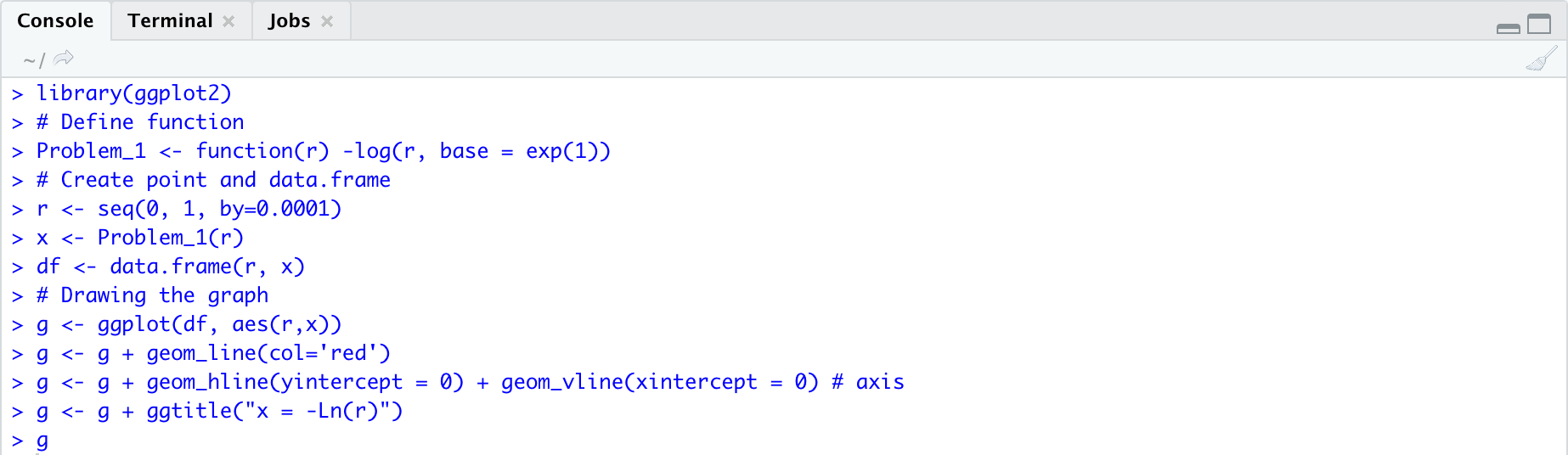
According to the graph, we can easily know that $x \in [0, \infty)$, which means $x$ has the maximum value when $r = 1$ and $x$ has the minimum value when $r$ is close to 0. But $r$ could not be 0 and has a very low probability to make $x$ larger than 10. Using the Data Analysis -> Descriptive Statistics tool to create a descriptive table. Combining the descriptive table and the graph, I set the bin from 0.1 to 9.9 with the first Left End 0 and the last Right End 10.
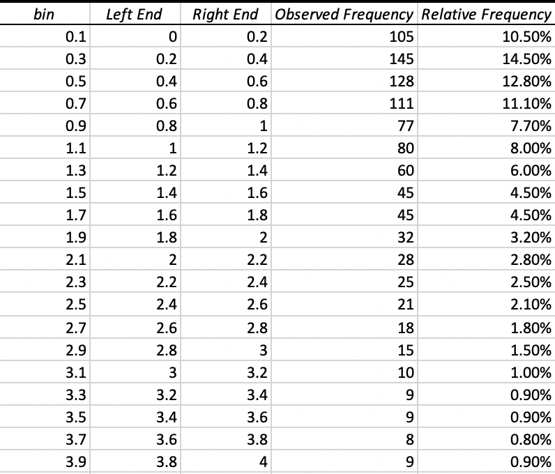
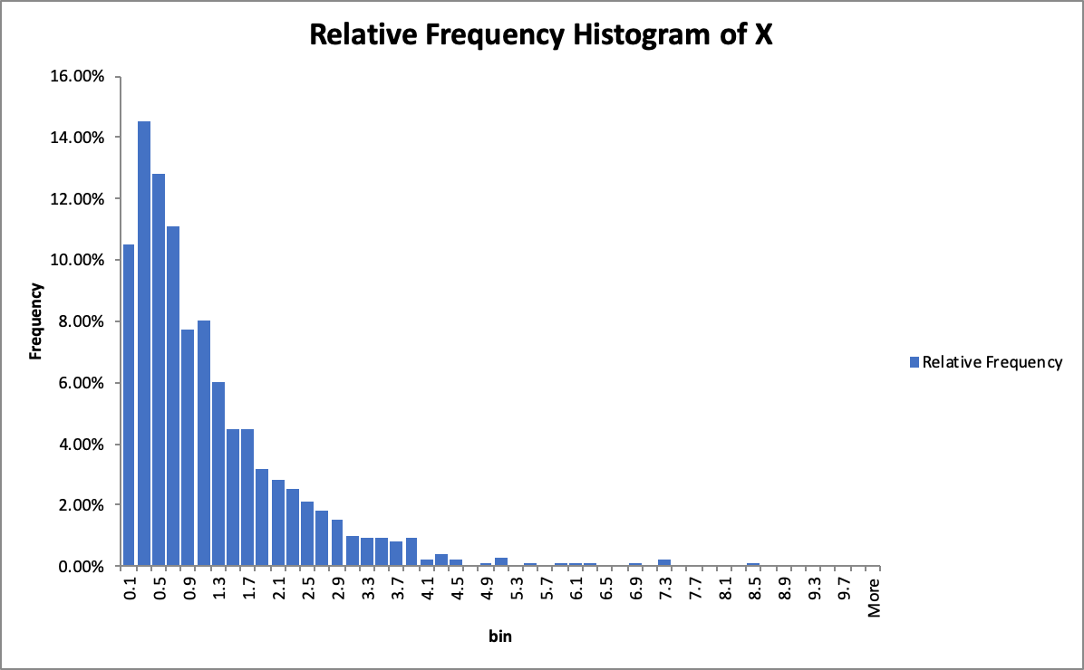
Second, using the Data Analysis -> Histogram to create a frequency histogram and calculate the Relative Frequency. After modifying the frequency histogram, I get the Relative Frequency Histogram of X.
2
According to the Central Limit Theorem, if the sample size is large enough (generally at least 30, but depends on the actual distribution), the sampling distribution of the mean is approximately normal, regardless of the distribution of the population. Therefore, $r$ with 1,000 samples is approximately normal.
Assume $X$ is an exponential distribution since the relative frequency histogram of X is similar to exponential distribution.
5
According to the following mathematic functions and Excel function:
- $EV[X] = 1/\lambda$
- $V[X] = 1/\lambda^2$
- $\displaystyle \chi^2 = \sum^n_{i=1}\frac{(O_i-E_i)^2}{E_i}$
- =EXPON.DIST(x,$\lambda$,cumulative)
I got the Exponential Probability, Expected Frequency, and $\chi^2$. Then I make a hypothesis and calculate:
- $H_0$: Data belongs to the Exponential Distribution.
- $H_1$: Data does not belongs to the Exponential Distribution.
- P-value: area under the chi-squared distribution and on the right of the test statistic.
- DF = n - k - 1 = 48
Since the P-value does not less than 0.05, we do not reject the $H_0$ hypothesis. There is no sufficient evidence to reject the fact that $X$ belongs to the Exponential Distribution.
6
I learned a very important point from this experiment is NEVER fix the random value. First time I generated 1,000 $r$ by Analysis Tool -> Random Number Generation. All of the values of $r$ are fixed resulting in I get a frequency histogram of X that seems like a Gamma Distribution. No matter what I tried, for example, check and improve Excel functions, it never shows the right answer. Once, it even rejects my $H_0$ Hypothesis that the distribution of $X$ is Exponential with a very low probability to happen.
Another thing I learned is the mathematical theory. Initially, I cannot figure out why the function $x = -Ln(r)$, as a Logarithm, is not a Lognormal Distribution. Especially when I saw that sentence from Statistics, Data Analysis, and Decision Modeling, Fifth Edition: “If the natural logarithm of a random variable 𝑋 is normal, then 𝑋 has a lognormal distribution.”, which haunts me several days. Finally I realized that what pursue is not the distribution of independent variable of $x = -Ln(r)$, instead, it is the dependent variable of $x = -Ln(r)$.
Problem 2
Questions
- Create a relative frequency histogram of $X$.
- Select a probability distribution that, in your judgement, is the best fit for $X$.
- Support your assertion above by creating a probability plot for X.
- Support your assertion above by performing a Chi-squared test of best fit with a 0.05 level of significance.
- In the word document, describe your methodologies and conclusions.
- In the word document, explain what you have learned from this experiment.
Solutions
1
First of all, using the Excel function Rand() to generate 1,000 uniform variables between $[0, 1]$. Then I draw a graph in RStudio for $x = -Ln(r)$.
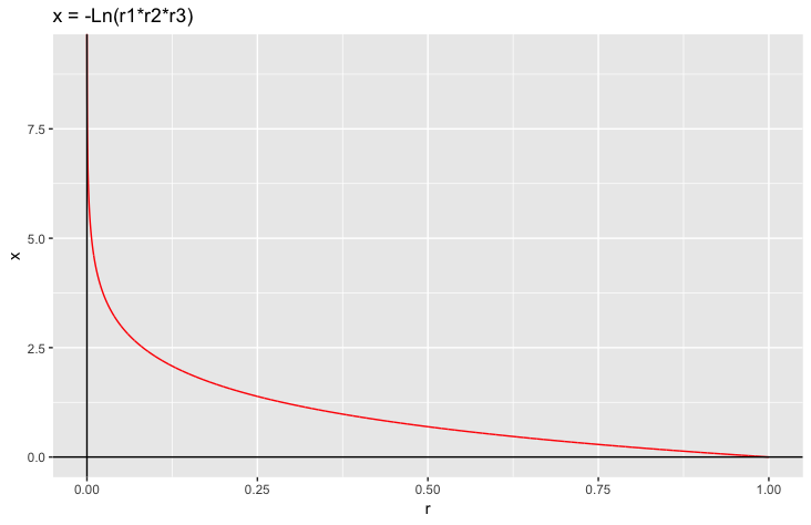
According to the graph, we can easily know that $x \in [0, \infty)$, which means $x$ has the maximum value when $r_1 \times r_2 \times r_3 = 1$ and $x$ has the minimum value when $r_1 \times r_2 \times r_3$ is close to 0. But $r_1 \times r_2 \times r_3$ could not be 0 and has a relative high probability, in comparison to problem, to make $x$ larger than 10. Using the Data Analysis -> Descriptive Statistics tool to create a descriptive table. Combining the descriptive table and the graph, I set the bin from 0.2 to 15 with the first Left End 0 and the last Right End 15.1.
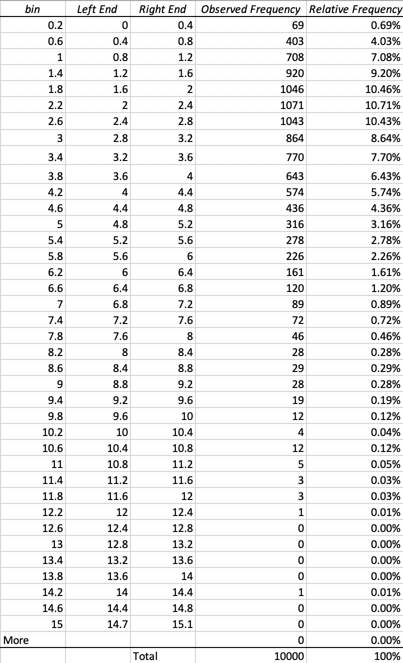
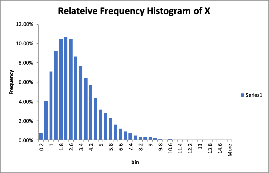
Second, using the Data Analysis -> Histogram to create a frequency histogram and calculate the Relative Frequency. After modifying the frequency histogram, I get the Relative Frequency Histogram of X.
2
Assume $X$ is an Gamma distribution since the relative frequency histogram of X is similar to Gamma distribution.
5
According to the following mathematic functions and Excel function:
- With a shape parameter $k$ and a scale parameter $θ$.
- With a shape parameter $α = k$ and an inverse scale parameter $β = 1/θ$, called a rate parameter.
- With a shape parameter $k$ and a mean parameter $μ = kθ = α/β$.
- For large $k$ the gamma distribution converges to normal distribution with mean $μ = kθ$ and variance $σ^2 = kθ^2$.
- $\displaystyle \chi^2 = \sum^n_{i=1}\frac{(O_i-E_i)^2}{E_i}$
Therefore:
- $\sigma^2 = \mu \times \theta \Rightarrow \theta = \sigma^2/\mu$
- $\beta = \mu/\sigma^2$
- $\alpha = \mu \times \beta$
I got the Gamma Probability, Expected Frequency, and $\chi^2$. Then I make a hypothesis and calculate:
- $H_0$: Data belongs to the Gamma Distribution.
- $H_1$: Data does not belongs to the Gamma Distribution.
- P-value: area under the chi-squared distribution and on the right of the test statistic.
- DF = n - k - 1 = 35
Since the P-value does not less than 0.05, we do not reject the $H_0$ hypothesis. There is no sufficient evidence to reject the fact that $X$ belongs to the Gamma Distribution.
Problem 3
Questions
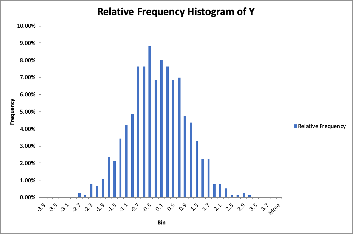
- Create a relative frequency histogram of $Y$.
- Select a probability distribution that, in your judgement, is the best fit for $Y$.
- Support your assertion above by creating a probability plot for $Y$.
- Support your assertion above by performing a Chi-squared test of best fit with a 0.05 level of significance.
- In the word document, describe your methodologies and conclusions.
- In the word document, explain what you have learned from this experiment.
Solutions
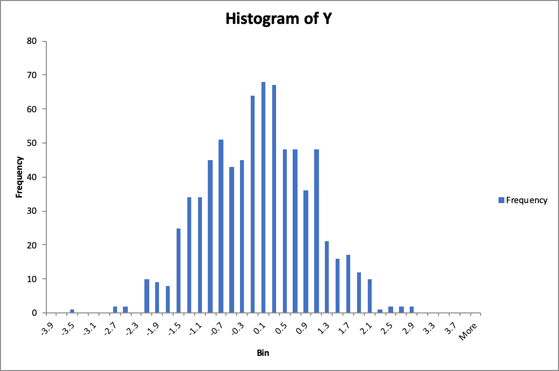
1
2
Standard Normal Distribution
3
5
- if $X \sim N(\mu, \sigma^2)$, then $\displaystyle Z = \frac{(X - \mu)}{\sigma} \sim N(0, 1)$
- $\displaystyle \chi^2 = \sum^n_{i=1}\frac{(O_i-E_i)^2}{E_i}$
$H_0$: Data belongs to the Standard Normal Distribution
$H_1$: Data is not belongs to the Standard Normal Distribution
P-value: area under the chi-squared distribution and on the right of the test statistic
DF = n - k - 1
P-value
Reject
Since the P-value is less than 0.05, we reject the $H_0$ hypothesis.
There is no sufficient evidence to support the fact that $$ belongs to the Standard Normal Distribution
Problem 4
Questions
- Estimate the expected value and the standard deviation of $W$.
- Select a probability distribution that, in your judgement, is the best fit for $W$.
- Support your assertion above by performing a Chi-squared test of best fit with a 0.05 level of significance.
- As the number of iterations $M$ becomes larger, the values $W$ will approach a certain limiting value. Investigate this limiting value of $W$ by completing the following table and plotting $W$ versus $M$. What value do you propose for the limiting value that $W$ approaches to?
Solutions
1 & 4
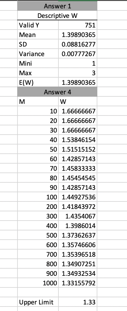
2
Normal Distribution
Summary
In the word document, summarize and conceptualize your findings in parts 1 – 4 above by filling the blanks in the sentences below:
- If $r$ is a standard uniform random variable, then $-Ln(r)$ has the Exponential Distribution probability distribution.
- The sum of three independent and identically distributed Exponential random variables has the Gamma probability distribution.
- The output of the algorithm of problem 3 has a Normal Distribution probability distribution.
- In step 2 of the algorithm of problem 3, random variables $X_1$ and $X_2$, each of whose probability distribution is Exponential Distribution are used to generate a random value $Y$ that has the Normal probability distribution.
- The random value $W$ that was discussed in problem 4, has the Normal probability distribution. The expected value of $W$ is: 1.33.
Reference
James R. Evans(2013). Statistics, Data Analysis, and Decision Modeling, Fifth Edition. Copyright ©2013 Pearson Education, Inc. publishing as Prentice Hall
Normal distribution. Retrieved from https://www3.nd.edu/~rwilliam/stats1/x21.pdf