Udacity Data Structure & Algorithms
Reference
Udacity Data Structure & Algorithms Nanodegree
Big-O Cheatsheet
Python Complexities
Introduction
How to Solve Problems
Efficiency (Complexity)
Efficiency
We said earlier that this Nanodegree program is about how to write code to solve problems and to do so efficiently.
In the last section, we looked at some basic aspects of solving problems—but we didn’t really think too much about whether our solutions were efficient.
Space and time
When we refer to the efficiency of a program, we aren’t just thinking about its speed—we’re considering both the time it will take to run the program and the amount of space the program will require in the computer’s memory. Often there will be a trade-off between the two, where you can design a program that runs faster by selecting a data structure that takes up more space—or vice versa.
Algorithms
An algorithm is essentially a series of steps for solving a problem. Usually, an algorithm takes some kind of input (such as an unsorted list) and then produces the desired output (such as a sorted list).
For any given problem, there are usually many different algorithms that will get you to exactly the same end result. But some will be much more efficient than others. To be an effective problem solver, you’ll need to develop the ability to look at a problem and identify different algorithms that could be used—and then contrast those algorithms to consider which will be more or less efficient.
But computers are so fast!
Sometimes it seems like computers run programs so quickly that efficiency shouldn’t really matter. And in some cases, this is true—one version of a program may take 10 times longer than another, but they both still run so quickly that it has no real impact.
But in other cases, a small difference in how your code is written—or a tiny change in the type of data structure you use—can mean the difference between a program that runs in a fraction of a millisecond and a program that takes hours (or even years!) to run.
In thinking about the efficiency of a program, which is more important: The time the program will take to run, or the amount of space the program will require?
The time complexity of the problem is more important
The space complexity of the problem is more important
It really depends on the problem
Quantifying Efficiency
It’s fine to say “this algorithm is more efficient than that algorithm”, but can we be more specific than that? Can we quantify things and say how much more efficient the algorithm is?
Let’s look at a simple example, so that we have something specific to consider.
Here is a short (and rather silly) function written in Python:
1 | def some_function(n): |
What does it do?
Adds 2 to the given input.
Adds 200 to the given input.
Adds 100 to the given input.
Now how about this one?
1 | def other_function(n): |
What does it do?
Adds 2 to the given input.
Adds 200 to the given input.
Adds 100 to the given input.
So these functions have exactly the same end result. But can you guess which one is more efficient?
Here they are next to each other for comparison:
1 | def some_function(n): |
some_function is more efficient
other_function is more efficient
They have exactly the same efficiency.
Although the two functions have the exact same end result, one of them iterates many times to get to that result, while the other iterates only a couple of times.
This was admittedly a rather impractical example (you could skip the for loop altogether and just add 200 to the input), but it nevertheless demonstrates one way in which efficiency can come up.
Counting lines
With the above examples, what we basically did was count the number of lines of code that were executed. Let’s look again at the first function:
1 | def some_function(n): |
There are four lines in total, but the line inside the for loop will get run twice. So running this code will involve running 5 lines.
Now let’s look at the second example:
1 | def other_function(n): |
In this case, the code inside the loop runs 100 times. So running this code will involve running 103 lines!
Counting lines of code is not a perfect way to quantify efficiency, and we’ll see that there’s a lot more to it as we go through the program. But in this case, it’s an easy way for us to approximate the difference in efficiency between the two solutions. We can see that if Python has to perform an addition operation 100 times, this will certainly take longer than if it only has to perform an addition operation twice!
Input size and efficiency
Here’s one of our functions from the last page:
1 | def some_function(n): |
Suppose we call this function and give it the value 1, like this:
1 | some_function(1) |
And then we call it again, but give it the input 1000:
1 | some_function(1000) |
Will this change the number of lines of code that get run?
Yes — some_function(1000) will involve running more lines of code.
Yes — some_function(1) will involve running more lines of code.
No — the same number of lines will run in both cases.
Now, here’s a new function:
1 | def say_hello(n): |
Suppose we call it like this:
1 | say_hello(3) |
And then we call it like this:
1 | say_hello(1000) |
Will this change the number of lines of code that get run?
Yes — say_hello(3) will involve running more lines of code.
Yes — say_hello(1000) will involve running more lines of code.
No — the same number of lines will run in both cases.
This highlights a key idea:
As the input to an algorithm increases, the time required to run the algorithm may also increase.
Notice that we said may increase. As we saw with the above examples, input size sometimes affects the run-time of the program and sometimes doesn’t—it depends on the program.
The rate of increase
Let’s look again at this function from above:
1 | def say_hello(n): |
Below are some different function calls. Match each one with the number of lines of code that will get run.
| FUNCTION CALL | HOW MANY LINES GET RUN? |
|---|---|
| say_hello(1) | 3 |
| say_hello(2) | 4 |
| say_hello(3) | 5 |
| say_hello(4) | 6 |
Here’s another question about that same function (from the above exercise). When we increase the size of the input n by 1, how many more lines of code get run?
When n goes up by 1, the number of lines run also goes up by 1.
When n goes up by 1, the number of lines run goes up by 2.
When n goes up by 1, the number of lines run goes up by 4.
So here’s one thing that we know about this function: As the input increases, the number of lines executed also increases.
But we can go further than that! We can also say that as the input increases, the number of lines executed increases by a proportional amount. Increasing the input by 1 will cause 1 more line to get run. Increasing the input by 10 will cause 10 more lines to get run. Any change in the input is tied to a consistent, proportional change in the number of lines executed. This type of relationship is called a linear relationship, and we can see why if we graph it:

Derivative of “Comparison of computational complexity” by Cmglee. Used under CC BY-SA 4.0.
The horizontal axis, n, represents the size of the input (in this case, the number of times we want to print "Hello!").
The vertical axis, N, represents the number of operations that will be performed. In this case, we’re thinking of an “operation” as a single line of Python code (which is not the most accurate, but it will do for now).
We can see that if we give the function a larger input, this will result in more operations. And we can see the rate at which this increase happens—the rate of increase is linear. Another way of saying this is that the number of operations increases at a constant rate.
If that doesn’t quite seem clear yet, it may help to contrast it with an alternative possibility—a function where the operations increase at a rate that is not constant.
Now here’s a slightly modified version of the say_hello function:
1 | def say_hello(n): |
Notice that it has a nested loop (a for loop inside another for loop!).
Below are some function calls. Match each one with the number of times "Hello!" will get printed.
| FUNCTION CALL | HOW MANY TIMES WILL IT PRINT HELLO? |
|---|---|
| say_hello(1) | 1 |
| say_hello(2) | 4 |
| say_hello(3) | 9 |
| say_hello(4) | 16 |
Looking at the say_hello function from the above exercise, what can we say about the relationship between the input, n, and the number of times the function will print "Hello!"?
The function will always print "Hello!" the same number of times (changing n doesn’t make a difference).
The function will print "Hello!" exactly n times (so say_hello(2) will print "Hello!" twice).
The function will print "Hello!" exactly n-squared times (so say_hello(2) will print "Hello!" 2*2 or four times).
Notice that when the input goes up by a certain amount, the number of operations goes up by the square of that amount. If the input is $2$, the number of operations is $2^2$ or $4$. If the input is $3$, the number of operations is $3^2$ or $9$.
To state this in general terms, if we have an input, $n$, then the number of operations will be $n^2$. This is what we would call a quadratic rate of increase.
Let’s compare that with the linear rate of increase. In that case, when the input is $n$, the number of operations is also $n$.
Let’s graph both of these rates so we can see them together:

Our code with the nested for loop exhibits the quadratic $n^2$ relationship on the left. Notice that this results in a much faster rate of increase. As we ask our code to print larger and larger numbers of "Hellos!", the number of operations the computer has to perform shoots up very quickly—much more quickly than our other function, which shows a linear increase.
This brings us to a second key point. We can add it to what we said earlier:
As the input to an algorithm increases, the time required to run the algorithm may also increase—and different algorithms may increase at different rates.
Notice that if n is very small, it doesn’t really matter which function we use—but as we put in larger values for n, the function with the nested loop will quickly become far less efficient.
We’ve looked here only at a couple of different rates—linear and quadratic. But there are many other possibilities. Here we’ll show some of the common types of rates that come up when designing algorithms:

We’ll look at some of these other orders as we go through the class. But for now, notice how dramatic a difference there is here between them! Hopefully you can now see that this idea of the order or rate of increase in the run-time of an algorithm is an essential concept when designing algorithms.
Order
We should note that when people refer to the rate of increase of an algorithm, they will sometimes instead use the term order. Or to put that another way:
The rate of increase of an algorithm is also referred to as the order of the algorithm.
For example, instead of saying “this relationship has a linear rate of increase”, we could instead say, “the order of this relationship is linear”.
On the next page, we’ll introduce something called Big O Notation, and you’ll see that the “O” in the name refers to the order of the rate of increase.
Big O Notation
When describing the efficiency of an algorithm, we could say something like “the run-time of the algorithm increases linearly with the input size”. This can get wordy and it also lacks precision. So as an alternative, mathematicians developed a form of notation called big O notation.
The “O” in the name refers to the order of the function or algorithm in question. And that makes sense, because big O notation is used to describe the order—or rate of increase—in the run-time of an algorithm, in terms of the input size (n).
In this next video, Brynn will show some different examples of what the notation would actually look like in practice. This likely won’t “click” for you right away, but don’t worry—once you’ve gotten some experience applying it to real problems, it will be much more concrete.
- Capital
O - Parentheses
() - Algebraic expression like
nn: represents the length of an input to your function
Examples:
- $O(log(n))$
- $O(n)$
- $O(n^3)$
- $O(n^2)$
- $O(1)$
- $O(\sqrt{n})$
- $O(nlog(n))$
When you see some Big O notation, such as O(2n + 2), what does n refer to?
The amount of time (usually in milliseconds) your algorithm will take to run.
The amount of memory (usually in kilobytes) that your algorithm will require.
The length of the input to your algorithm.
The length of the output from your algorithm.
Here’s the cipher pseudocode Brynn showed in the video:
1 | function decode(input): |
Brynn estimated the efficiency as O(2n + 2). Suppose the input string is "jzqh". What is n in this case?
1
2
3
4
5
Which of these is the same as O(1)?
O(0n + 1)
O(n + 1))
O(n)
O(n + 0)
Here’s one of the functions we looked at on the last page:
1 | def say_hello(n): |
Which of these would best approximate the efficiency using big O notation?
$\displaystyle n$
$\displaystyle n^2$
$\displaystyle log(n)$
$\displaystyle 2^n$
$\displaystyle \sqrt{n}$
Here’s the other function we looked at on the last page:
1 | def say_hello(n): |
Again, which of these would best approximate the efficiency using big O notation?
$\displaystyle n$
$\displaystyle n^2$
$\displaystyle log(n)$
$\displaystyle 2^n$
$\displaystyle \sqrt{n}$
In the examples we’ve looked at here, we’ve been approximating efficiency by counting the number of lines of code that get executed. But when we are thinking about the run-time of a program, what we really care about is how fast the computer’s processor is, and how many operations we’re asking the processor to perform. Different lines of code may demand very different numbers of operations from the computer’s processor. For now, counting lines will work OK as an approximation, but as we go through the course you’ll see that there’s a lot more going on under the surface.
Worst Case and Approximation
Suppose that we analyze an algorithm and decide that it has the following relationship between the input size, n, and the number of operations needed to carry out the algorithm:
$$N = n^2 +5$$
Where $n$ is the input size and $N$ is the number of operations required.
For example, if we gave this algorithm an input of $2$, the number of required operations would be $2^2 +5$ or simply $9$.
Below are some other possible values for the input $(n)$. For each input, what does $n^2 + 5$ evaluate to?
| INPUT | NUMBER OF OPERATIONS |
|---|---|
| 5 | 30 |
| 10 | 105 |
| 25 | 630 |
| 100 | 10005 |
The thing to notice in the above exercise, is this: In $n^2 +5$, the $5$ has very little impact on the total efficiency—especially as the input size gets larger and larger. Asking the computer to do 10,005 operations vs. 10,000 operations makes little difference. Thus, it is the $n^2$ that we really care about the most, and the $+5$ makes little difference.
Most of the time, when analyzing the efficiency of an algorithm, the most important thing to know is the order. In other words, we care a lot whether the algorithm’s time-complexity has a linear order or a quadratic order (or some other order). This means that very often (in fact, most of the time) when you are asked to analyze an algorithm, you can do so by making an approximation that significantly simplifies things. In this next video, Brynn will discuss this concept and show how it’s used with Big O Notation.
By approximating, we’re really say:
“Some number of computations must be performed for EACH letter in the input.”
Efficiency Practice
What is the run time analysis of the following code:
1 | def main(x,y): |
$O(log(n))$
$O(n)$
$O(n^2)$
$O(1)$
What is the run time analysis of the following code:
1 | def main(list_1,list_2): |
$O(log(n))$
$O(n)$
$O(n^2)$
$O(1)$
What is the simplification of this run time analysis: 4n^2 + 3n + 7 ?
$4n^2+3n$
$4n^2 + 3n + 7$
$4n^2$
$n^2$
Resources
Space Complexity
Space Complexity Examples
When we refer to space complexity, we are talking about how efficient our algorithm is in terms of memory usage. This comes down to the datatypes of the variables we are using and their allocated space requirements. In Python, it’s less clear how to do this due to the underlying data structures using more memory for house keeping functions (as the language is actually written in C).
For example, in C/C++, an integer type takes up 4 bytes of memory to store the value, but in Python 3 an integer takes 14 bytes of space. Again, this extra space is used for housekeeping functions in the Python language.
For the examples of this lesson we will avoid this complexity and assume the following sizes:
| Type | Storage size |
|---|---|
| char | 1 byte |
| bool | 1 byte |
| int | 4 bytes |
| float | 4 bytes |
| double | 8 bytes |
It is also important to note that we will be focusing on just the data space being used and not any of the environment or instructional space.
Example 1
1 | def our_constant_function(): |
So in this example we have four integers (x, y, z and answer) and therefore our space complexity will be 4*4 = 16 bytes. This is an example of constant space complexity, since the amount of space used does not change with input size.
Example 2
1 | def our_linear_function(n): |
So in this example we have two integers (n and counter) and an expanding list, and therefore our space complexity will be 4*n + 8 since we have an expanding integer list and two integer data types. This is an example of linear space complexity.
Project: Unscramble Computer Science Problems
Deconstruct a series of open-ended problems into smaller components (e.g, inputs, outputs, series of functions)
Investigating Texts and Calls
Project Overview
In this project, you will complete five tasks based on a fabricated set of calls and texts exchanged during September 2016. You will use Python to analyze and answer questions about the texts and calls contained in the dataset. Lastly, you will perform run time analysis of your solution and determine its efficiency.
What will I learn?
In this project, you will:
- Apply your Python knowledge to breakdown problems into their inputs and outputs.
- Perform an efficiency analysis of your solution.
- Warm up your Python skills for the course.
Why this Project?
You’ll apply the skills you’ve learned so far in a more realistic scenario. The five tasks are structured to give you experience with a variety of programming problems. You will receive code review of your work; this personal feedback will help you to improve your solutions.
Step 1 - Download the Files
Download and open the zipped folder here. In the folder you will find five python files Task0.py, Task1.py, …,Task4.py and two csv files calls.csv and texts.csv
About the data
The text and call data are provided in csv files.
The text data (text.csv) has the following columns: sending telephone number (string), receiving telephone number (string), timestamp of text message (string).
The call data (call.csv) has the following columns: calling telephone number (string), receiving telephone number (string), start timestamp of telephone call (string), duration of telephone call in seconds (string)
All telephone numbers are 10 or 11 numerical digits long. Each telephone number starts with a code indicating the location and/or type of the telephone number. There are three different kinds of telephone numbers, each with a different format:
- Fixed lines start with an area code enclosed in brackets. The area codes vary in length but always begin with 0. Example: “(022)40840621”.
- Mobile numbers have no parentheses, but have a space in the middle of the number to help readability. The mobile code of a mobile number is its first four digits and they always start with 7, 8 or 9. Example: “93412 66159”.
- Telemarketers’ numbers have no parentheses or space, but start with the code 140. Example: “1402316533”.
Step 2 - Implement the Code
Complete the five tasks (Task0.py, Task1.py, …,Task4.py). Do not change the data or instructions, simply add your code below what has been provided. Include all the code that you need for each task in that file.
In Tasks 3 and 4, you can use in-built methods sorted() or list.sort() for sorting which are the implementation of Timsort and Samplesort, respectively. Both these sorting methods have a worst-case time-complexity of O(n log n). Check the below links to learn more about these methods:
- How to use the above methods - https://docs.python.org/3/howto/sorting.html
- Complexity analysis of Timsort and Samplesort - http://svn.python.org/projects/python/trunk/Objects/listsort.txt
The solution outputs for each file should be the print statements described in the instructions. Feel free to use other print statements during the development process, but remember to remove them for submission - the submitted files should print only the solution outputs.
Step 3 - Calculate Big O
Once you have completed your solution for each problem, perform a run time analysis (Worst Case Big-O Notation) of your solution. Document this for each problem and include this in your submission.
Step 4 - Check again Rubric and Submit
Use the rubric to check your work before submission. A Udacity Reviewer will give feedback on your work based on this rubric and will leave helpful comments on your code.
Data Types and Operators
Python Built-in Data Structures
Data structures are containers that can include different data types.
- Types of Data Structures: Lists, Tuples, Sets, Dictionaries, Compound Data Structures.
- All data structures are also data types.
Control Flow
Functions
Scripting
Advanced Topics
Data Structures
Arrays and Linked Lists
Why data structures?
Data structures are containers that organize and group data together in different ways. When you write code to solve a problem, there will always be data involved—and how you store or structure that data in the computer’s memory can have a huge impact on what kinds of things you can do with it and how efficiently you can do those things.
In this section, we’ll start out by reviewing some basic data structures that you’re probably at least partly familiar with already.
Then, as we go on in the course, we’ll consider the pros and cons of using different structures when solving different types of problems.

There are numerous types of data structures, generally built upon simpler primitive data types:
- An array is a number of elements in a specific order, typically all of the same type (depending on the language, individual elements may either all be forced to be the same type, or may be of almost any type). Elements are accessed using an integer index to specify which element is required. Typical implementations allocate contiguous memory words for the elements of arrays (but this is not always a necessity). Arrays may be fixed-length or resizable.
- A linked list (also just called list) is a linear collection of data elements of any type, called nodes, where each node has itself a value, and points to the next node in the linked list. The principal advantage of a linked list over an array is that values can always be efficiently inserted and removed without relocating the rest of the list. Certain other operations, such as random access to a certain element, are however slower on lists than on arrays.
- A record (also called tuple or struct) is an aggregate data structure. A record is a value that contains other values, typically in fixed number and sequence and typically indexed by names. The elements of records are usually called fields or members.
- A union is a data structure that specifies which of a number of permitted primitive types may be stored in its instances, e.g. float or long integer. Contrast with a record, which could be defined to contain a float and an integer; whereas in a union, there is only one value at a time. Enough space is allocated to contain the widest member datatype.
- A tagged union (also called variant, variant record, discriminated union, or disjoint union) contains an additional field indicating its current type, for enhanced type safety.
- An object is a data structure that contains data fields, like a record does, as well as various methods which operate on the data contents. An object is an in-memory instance of a class from a taxonomy. In the context of object-oriented programming, records are known as plain old data structures to distinguish them from objects.[11]
In addition, graphs and binary trees are other commonly used data structures.
Collections
Many collections define a particular linear ordering, with access to one or both ends. The actual data structure implementing such a collection need not be linear—for example, a priority queue is often implemented as a heap, which is a kind of tree. Important linear collections include:
Array
- One-dimensional arrays: A one-dimensional array (or single dimension array) is a type of linear array. Accessing its elements involves a single subscript which can either represent a row or column index.
- Multidimensional arrays
Arrays
An array has some things in common with a list. In both cases:
- There is a collection of items
- The items have an order to them
One of the key differences is that arrays have indices, while lists do not.
To understand this, it helps to know how arrays are stored in memory. When an array is created, it is always given some initial size—that is, the number of elements it should be able to hold (and how large each element is). The computer then finds a block of memory and sets aside the space for the array.
Importantly, the space that gets set aside is one, continuous block. That is, all of the elements of the array are contiguous, meaning that they are all next to one another in memory.
Another key characteristic of an array is that all of the elements are the same size.
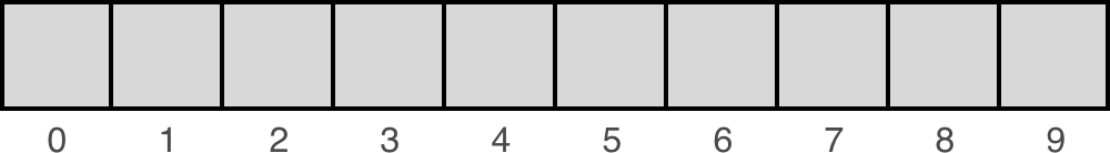
When we represent an array visually, we often draw it as a series of boxes that are all of the same size and all right next to one another:

Because all of the elements are 1) next to one another and 2) the same size, this means that if we know the location of the first element, we can calculate the location of any other element.
For example, if the first element in the array is at memory location 00 and the elements are 24 bytes, then the next element would be at location 00 + 24 = 24. And the one after that would be at 24 + 24 = 48, and so on.
Since we can easily calculate the location of any item in the array, we can assign each item an index and use that index to quickly and directly access the item.
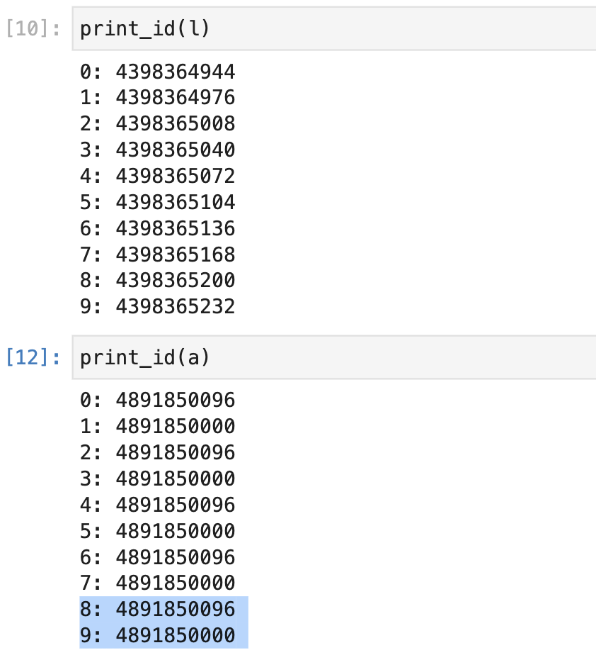
1 | import numpy as np |
As you can see, the array uses two consecutive blocks of memory to store the numbers from 0 to 9 while the elements of a Python list are contiguous in memory, and they can be accessed using an index.
Lists
In contrast, the elements of a list may or may not be next to one another in memory! For example, later in this lesson we’ll look at linked lists, where each list item points to the next list item—but where the items themselves may be scattered in different locations of memory. In this case, knowing the location of the first item in the list does not mean you can simply calculate the location of the other items. This means we cannot use indices to directly access the list items as we would in an array. We’ll explore linked lists in more detail shortly.
Python lists
In Python, we can create a list using square brackets [ ]. For example:
1 | >>> my_list = ['a', 'b', 'c'] |
And then we can access an item in the list by providing an index for that item:
1 | >>> my_list[0] |
But wait, didn’t we just say that lists don’t have indices!? This seems to directly contradict that distinction.
The reason for this confusion is simply one of terminology. The earlier description we gave of lists is correct _in general_—that is, usually when you hear someone refer to something as a “list”, that is what they mean. However, in Python the term is used differently.
We will not get into all of the details, but the important thing you need to know for this course is the following: If you were to look under the hood, you would find that a Python list is essentially implemented like an array (specifically, it behaves like a dynamic array, if you’re curious). In particular, the elements of a Python list are contiguous in memory, and they can be accessed using an index.
In addition to the underlying array, a Python list also includes some additional behavior. For example, you can use things like pop and append methods on a Python list to add or remove items. Using those methods, you can essentially utilize a Python list like a stack (which is another type of data structure we’ll discuss shortly).
In general, we will try to avoid using things like pop and append, because these are high-level language features that may not be available to you in other languages. In most cases, we will ignore the extra functionality that comes with Python lists, and instead use them as if they were simple arrays. This will allow you to see how the underlying data structures work, regardless of the language you are using to implement those structures.
Here’s the bottom line:
- Python lists are essentially arrays, but also include additional high-level functionality
- During this course, we will generally ignore this high-level functionality and treat Python lists as if they were simple arrays
This approach will allow you to develop a better understanding for the underlying data structures.
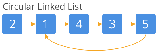
Linked List
In computer science, a linked list is a linear collection of data elements whose order is not given by their physical placement in memory. Instead, each element points to the next. It is a data structure consisting of a collection of nodes which together represent a sequence. In its most basic form, each node contains: data, and a reference (in other words, a link) to the next node in the sequence. This structure allows for efficient insertion or removal of elements from any position in the sequence during iteration. More complex variants add additional links, allowing more efficient insertion or removal of nodes at arbitrary positions. A drawback of linked lists is that access time is linear (and difficult to pipeline). Faster access, such as random access, is not feasible. Arrays have better cache locality compared to linked lists.

Code: Implement a Linked List
Implement a Linked List
Node
Code: Linked Lists Basics
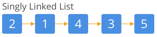
- Singly Linked List
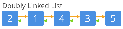
- Doubly Linked List
- Circular Linked List
Code: Linked List Practice
to_list()prepend()append()search()remove()pop()insert()size()
Code: Reverse a Linked List
__iter__()__repr__()prepend()reverse()
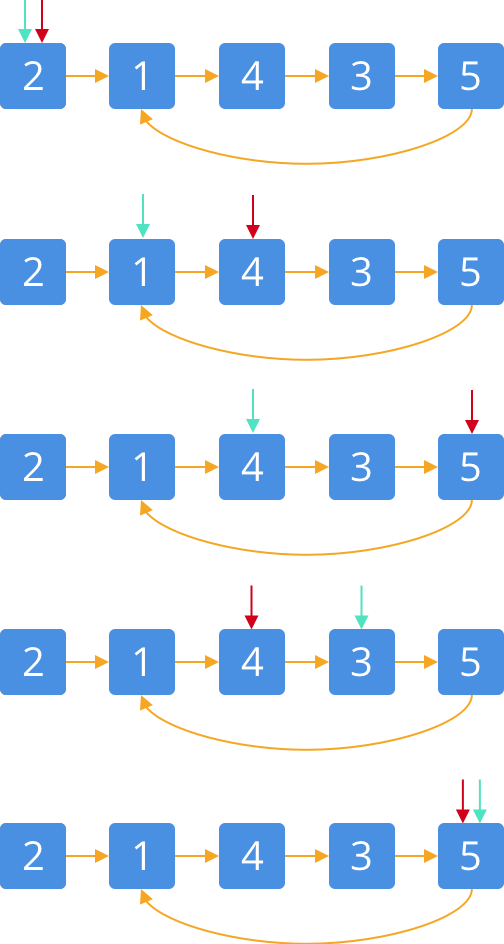
Code: Loop Detecting
Code: Merge, Sort, and Flatten a Nested Linked List
__getitem____len____add__copy()merge()quicksort()NestedLinkedList
Code: Even After Odd
create_linked_listfrom Python list to linked list
Code: Skip i, Delete j
Code: Swap Nodes
Array
Code: Add-One
- Add one to the last digit
Code: Duplicate Number
Code: Max Sum Subarray
Code: Pascal’s-Triangle
Stacks
Stacks: Last In, First Out
Queues: First In, First Out
Stack Introduction
Stack Details
Code: Implement a Stuck Using an Array
push- adds an item to the top of the stackpop- removes an item from the top of the stack (and returns the value of that item)size- returns the size of the stacktop- returns the value of the item at the top of stack (without removing that item)is_empty- returnsTrueif the stack is empty andFalseotherwise
Code: Implement a stack using a linked list
pushpopsizeis_empty
Code: Build Stack(Python List)
Code: Practice: Balanced Parentheses(Python List)
equation_checker
Code: Reverse Polish Notation
eval: and safety issues
Code: Reverse a Stack(Linked Lists)
reverse_stack
Code: Minimum Bracket Reversals(Linked List)
Queues
Stacks: Last In, First Out
Queues: First In, First Out
Queue: One way
Deque: Two ways
Code: Build a queue using an array
Build a queue using an array
- Unfinished
enqueuesizeis_emptyfrontdequeue_handle_queue_capacity_full
Code: Build a queue using a linked list
enqueuesizeis_emptydequeue
Code: Build a Queue From Stacks
enqueuesizedequeue
Code: Building a Queue From Python List
enqueuesizedequeue
Code: Reversed Queue(Node, Stack, Python List)
reverse_queue
Recursion
Introduction
We went over an example of the call stack when calling power_of_2(5) above. In this section, we’ll cover the limitations of recursion on a call stack. Run the cell below to create a really large stack. It should raise the error RecursionError: maximum recursion depth exceeded in comparison.
Python has a limit on the depth of recursion to prevent a stack overflow. However, some compilers will turn tail-recursive functions into an iterative loop to prevent recursion from using up the stack. Since Python’s compiler doesn’t do this, you’ll have to watch out for this limit.
Code: Recursion
Code: Factorial using recursion
Code: Reversing a String
Code: Palindrome
Code: Add One
Code: List Permutation
- Hard
Code: String Permutation
- Hard
Code: Keypad Combinations
- Hard, Unfinished
Code: Deep Reverse
- Intuitive
Code: Call stack
Code: Recurrence Relations
Binary Search
Code: Tower of Hanoi
- Hard
Code: Return Codes
- Hard
Code: Return Subsets
- Hard
Code: Staircase
509. Fibonacci Number
70. Climbing Stairs
1137. N-th Tribonacci Number
Code: Last Index
Trees
Trees
Tree
Branches
Leaf
Tree Basics
Tree is an extension of linked list.
Features
- Completely connected
- No Cycles
Tree Terminology
- Level
- Parent (P): Many children.
- Child (C): Only one parent.
- Descendant
- Leaf or external nodes. Others are internal nodes.
- Height: A leaf has the height of 0 and its parent has the height of 1.
- Depth: The opposite of Height.
Tree Traversal
Tree Traversal
- BFS: Breadth First Search
- Level Order Traversal
Depth-First Traversals
Tree Traversal
- DFS: Depth First Search
- Pre-Order: Check off the node as you see it before you traverse any further in the tree.
- In-Order: Check off all left children then move to parents.
- Post-Order: We won’t be able to check off a node until we’ve seen all off its descendants or we visited both of its children and returned.

Search and Delete
Binary tree is the simplest tree that has no more than 2 nodes.
Search: O(n)
Delete: O(n)
Insert
Insert: O(n)
Binary Search Trees
BSTs
BSTs are sorted.
Every nodes on the left is smaller than the parent; every value on the right of a particular is larger than the parent.
Search: log(n)
Insert: log(n)
BST Complications
Unbalanced Binary Tree
Search, Insert, Worst case O(n)
Practice Overview
Usage
- Database
- Machine Learning: Decision Tree
Code: Create a Binary Tree
Code: DFS
DFS with Node and Stack
Depth First Search Intro
Tree Setup
DFS uses a Stack
Coding Step by Step
DFS implementation with a Bug
Let’s look at a common error, an infinite loop, and explain why this is happening.
Tracking Additional Information in the Stack
Code that tracks the State in the Stack
Pre-Order DFS with Recursion Code Intro
DFS Pre-Order with Recursion Solution
In-Order and Post-Order Code Intro
In-Order and Post-Order Solution
Code: BFS
(Queue)
Breadth First Search intro
BFS is quiet useful especially for graph data structures and finding the shortest path.
Tree Setup
Queue for Breadth First Search
Code up a Queue
BFS Implementation Code intro
BFS Code Implementation Solution
BFS (Optional, Bonus): Print a Tree using BFS
Print a Tree Solution
Code: BST
Binary Search Tree Intro
Insert: log(n)
Search: log(n)
Delete: log(n)
Tree Setup
Insertion
Insertion Code Intro
Insertion Code Solution
Search
Search Code Intro
Search Code Solution
Delete
Code: Diameter of a Binary Tree
Code: Path From Root to Node
Unfinished
Interlude
Impostor Syndrome
Maps and Hashing
Introduction to Maps
Map is the same as dictionary.
Sets and Maps
Code: Exploring the Map Concepts
Introduction to Hashing
Hashing
O(1)
Collisions
Worst: O(m)
Ideally, 1 ~ 3 items in a bucket.
No prefect solution.
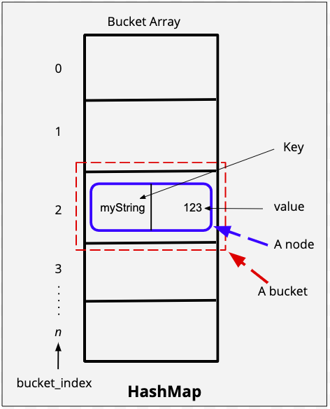
Hash Maps
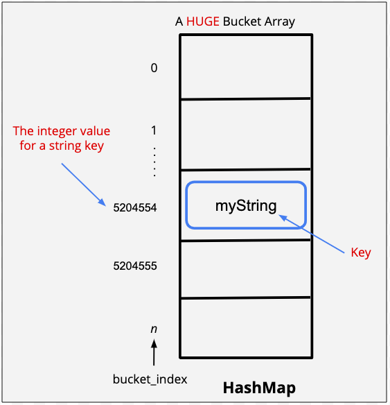
String Keys
Code: Hash Maps Notebook
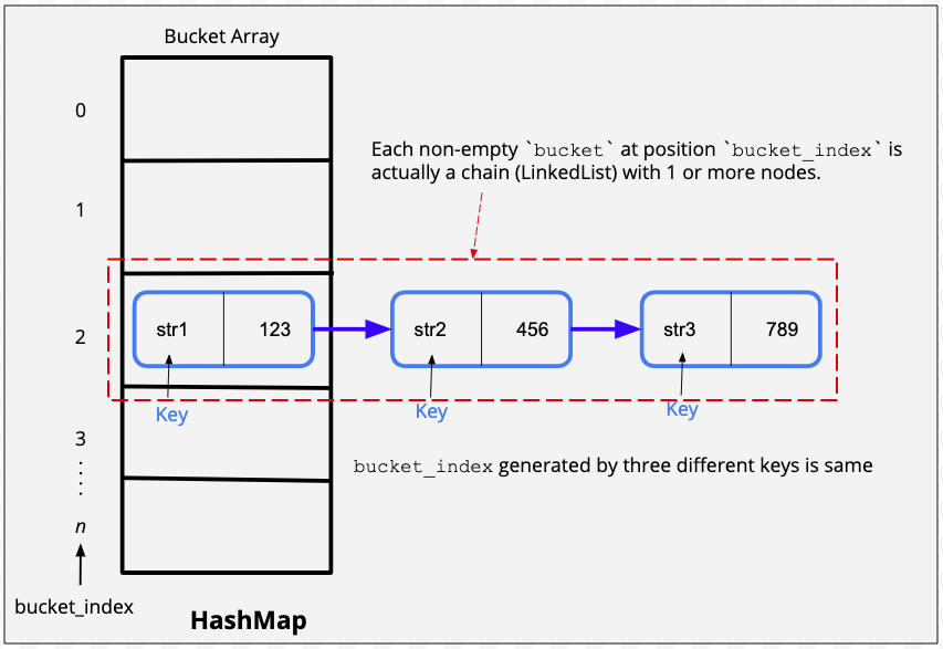
HashMap
- Hard
Because keys are unique, therefore…
Use keys as inputs to a hash function, then store the key value pair in the bucket of the hash value produced by the function.
A lot of research goes into figuring out good hash functions and this hash function is one of the most popular functions used for strings. We use prime numbers because the provide a good distribution. The most common prime numbers used for this function are 31 and 37.
Hash function for Strings
Compression Function
Collision Handling
There are two popular ways in which we handle collisions.
Separate chaining - Separate chaining is a clever technique where we use the same bucket to store multiple objects. The bucket in this case will store a linked list of key-value pairs. Every bucket has it’s own separate chain of linked list nodes.
Open Addressing - In open addressing, we do the following:
- If, after getting the bucket index, the bucket is empty, we store the object in that particular bucket
- If the bucket is not empty, we find an alternate bucket index by using another function which modifies the current hash code to give a new code. This process of finding an alternate bucket index is called probing. A few probing techniques are - linear probing, qudratic probing, or double hashing.
Code: Caching
Code: String Key Hash Table
Two Sum
Longest Consecutive Subsequence
128. Longest Consecutive Sequence
674. Longest Continuous Increasing Subsequence
300. Longest Increasing Subsequence
Unfinished
Project: Show Me the Data Structures
Data Structure Questions
For this project, you will answer the six questions laid out in the next sections. The questions cover a variety of topics related to the data structures you’ve learned in this course. You will write up a clean and efficient answer in Python, as well as a text explanation of the efficiency of your code and your design choices.
A qualified reviewer, such as a software or data engineer, will look over your answer and give you detailed, written feedback on areas you’re doing very well in and areas that could be improved. For example, is your solution the most efficient one possible? Are you doing a good job of explaining your thoughts? Is your code elegant and easy to read?
Feel free to write this code in your local development environment. In case you do not have the ability to use your local environment or wish to use the classroom to write your code a Jupyter notebook is provided below.
Problem 1: LRC Cache
Least Recently Used Cache
We have briefly discussed caching as part of a practice problem while studying hash maps.
The lookup operation (i.e., get()) and put() / set() is supposed to be fast for a cache memory.
While doing the get() operation, if the entry is found in the cache, it is known as a cache hit. If, however, the entry is not found, it is known as a cache miss.
When designing a cache, we also place an upper bound on the size of the cache. If the cache is full and we want to add a new entry to the cache, we use some criteria to remove an element. After removing an element, we use the put() operation to insert the new element. The remove operation should also be fast.
For our first problem, the goal will be to design a data structure known as a Least Recently Used (LRU) cache. An LRU cache is a type of cache in which we remove the least recently used entry when the cache memory reaches its limit. For the current problem, consider both get and set operations as an use operation.
Your job is to use an appropriate data structure(s) to implement the cache.
- In case of a
cache hit, yourget()operation should return the appropriate value. - In case of a
cache miss, yourget()should return -1. - While putting an element in the cache, your
put()/set()operation must insert the element. If the cache is full, you must write code that removes the least recently used entry first and then insert the element.
All operations must take O(1) time.
For the current problem, you can consider the size of cache = 5.
Here is some boiler plate code and some example test cases to get you started on this problem:
1 | class LRU_Cache(object): |
Problem 2: File Recursion
For this problem, the goal is to write code for finding all files under a directory (and all directories beneath it) that end with “.c”
Here is an example of a test directory listing, which can be downloaded here:
1 | ./testdir |
Python’s os module will be useful—in particular, you may want to use the following resources:
Note: os.walk() is a handy Python method which can achieve this task very easily. However, for this problem you are not allowed to use os.walk().
Here is some code for the function to get you started:
1 |
|
OS Module Exploration Code
1 | # Locally save and call this file ex.py ## |
Problem 3: Huffman Coding
Overview - Data Compression
In general, a data compression algorithm reduces the amount of memory (bits) required to represent a message (data). The compressed data, in turn, helps to reduce the transmission time from a sender to receiver. The sender encodes the data, and the receiver decodes the encoded data. As part of this problem, you have to implement the logic for both encoding and decoding.
A data compression algorithm could be either lossy or lossless, meaning that when compressing the data, there is a loss (lossy) or no loss (lossless) of information. The Huffman Coding is a lossless data compression algorithm. Let us understand the two phases - encoding and decoding with the help of an example.
A. Huffman Encoding
Assume that we have a string message AAAAAAABBBCCCCCCCDDEEEEEE comprising of 25 characters to be encoded. The string message can be an unsorted one as well. We will have two phases in encoding - building the Huffman tree (a binary tree), and generating the encoded data. The following steps illustrate the Huffman encoding:
Phase I - Build the Huffman Tree
A Huffman tree is built in a bottom-up approach.
- First, determine the frequency of each character in the message. In our example, the following table presents the frequency of each character.
| (Unique) Character | Frequency |
|---|---|
| A | 7 |
| B | 3 |
| C | 7 |
| D | 2 |
| E | 6 |
- Each row in the table above can be represented as a node having a character, frequency, left child, and right child. In the next step, we will repeatedly require to pop-out the node having the lowest frequency. Therefore, build and sort a list of nodes in the order lowest to highest frequencies. Remember that a list preserves the order of elements in which they are appended. We would need our list to work as a priority queue, where a node that has lower frequency should have a higher priority to be popped-out. The following snapshot will help you visualize the example considered above:
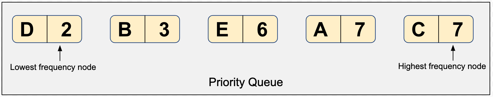
Can you come up with other data structures to create a priority queue? How about using a min-heap instead of a list? You are free to choose from anyone.
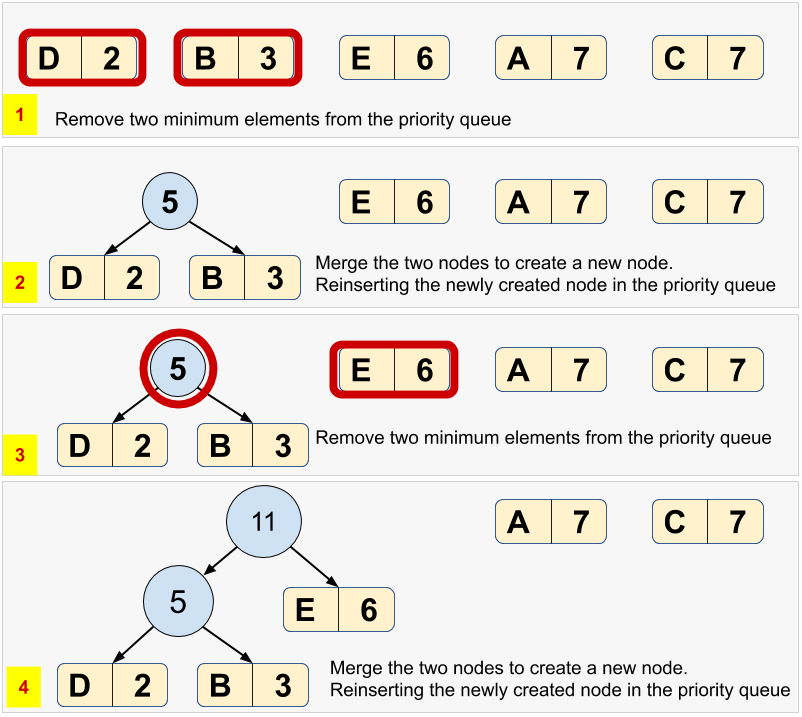
Pop-out two nodes with the minimum frequency from the priority queue created in the above step.
Create a new node with a frequency equal to the sum of the two nodes picked in the above step. This new node would become an internal node in the Huffman tree, and the two nodes would become the children. The lower frequency node becomes a left child, and the higher frequency node becomes the right child. Reinsert the newly created node back into the priority queue.
Do you think that this reinsertion requires the sorting of priority queue again? If yes, then a min-heap could be a better choice due to the lower complexity of sorting the elements, every time there is an insertion.
Repeat steps #3 and #4 until there is a single element left in the priority queue. The snapshots below present the building of a Huffman tree.
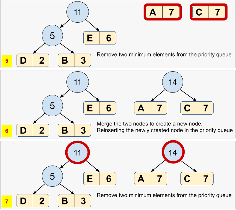
- For each node, in the Huffman tree, assign a bit
0for left child and a1for right child. See the final Huffman tree for our example:
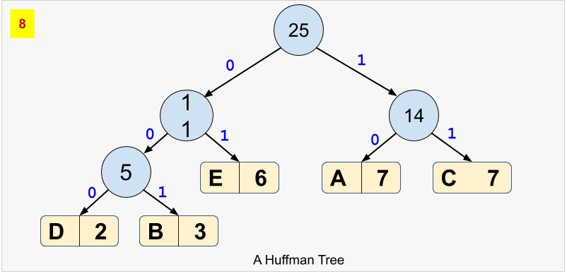
Phase II - Generate the Encoded Data
- Based on the Huffman tree, generate unique binary code for each character of our string message. For this purpose, you’d have to traverse the path from root to the leaf node.
| (Unique) Character | Frequency | Huffman Code |
|---|---|---|
| D | 2 | 000 |
| B | 3 | 001 |
| E | 6 | 01 |
| A | 7 | 10 |
| C | 7 | 11 |
Points to Notice
- Notice that the whole code for any character is not a prefix of any other code. Hence, the Huffman code is called a Prefix code.
- Notice that the binary code is shorter for the more frequent character, and vice-versa.
- The Huffman code is generated in such a way that the entire string message would now require a much lesser amount of memory in binary form.
- Notice that each node present in the original priority queue has become a leaf node in the final Huffman tree.
This way, our encoded data would be 1010101010101000100100111111111111111000000010101010101
B. Huffman Decoding
Once we have the encoded data, and the (pointer to the root of) Huffman tree, we can easily decode the encoded data using the following steps:
- Declare a blank decoded string
- Pick a bit from the encoded data, traversing from left to right.
- Start traversing the Huffman tree from the root.
- If the current bit of encoded data is
0, move to the left child, else move to the right child of the tree if the current bit is1. - If a leaf node is encountered, append the (alphabetical) character of the leaf node to the decoded string.
- If the current bit of encoded data is
- Repeat steps #2 and #3 until the encoded data is completely traversed.
You will have to implement the logic for both encoding and decoding in the following template. Also, you will need to create the sizing schemas to present a summary.
1 | import sys |
Visualization Resource
Check this website to visualize the Huffman encoding for any string message - Huffman Visualization!
Basic Algorithms
Basic Algorithms
Binary Search
Obviously, there is some randomness involved in this game, so in some cases you may run out of tries before guessing correctly. However, if you use a binary search strategy, you’ll find the number efficiently and win most of the time.
But before we look further into binary search, let’s first look at an alternative: Linear search.
Basic Binary Search Algorithm:
1 | class Solution: |
Linear search
Suppose that you have a dictionary of words and that you need to look up a particular word in this dictionary. However, this dictionary is a pretty terrible dictionary, because the words are all in a scrambled order (and not alphabetical as they usually are). What search strategy would you use to find the definition you’re looking for?
Because the words are in a random order, the best we can do is simply to go one by one, from the first page to the last page, in a sequential manner. Sounds tedious, right? This is called linear search. We have no idea about the order of the words, so we simply have to flip through the pages, one by one, until we find the word we are looking for.
With the example of the guessing game, you could use linear search there as well—by simply starting with 1 and guessing every number until you get to 100 (or rather, until you run out of tries and lose the game!).
What would the time complexity be for linear search?
(Think about the worst case scenario, where the word you’re looking for is on the last page of the dictionary.)
$O(1)$
$O(n)$
$O(log(n))$
$O(n^2)$
$O(2^n)$
$O(n!)$
Back to binary search
Now let’s consider a different scenario: Similar to the above, we have a dictionary and a word that we want to find in that dictionary. But this time, the dictionary is sorted in alphabetical order (just as you would expect from any decent dictionary). We still don’t know what page our word is on, so we’ll need to search for it—but the fact that the dictionary is sorted changes the strategy we should use.
You’re going to make your first guess about which page the word might be on. Then you’ll open the dictionary and take a look to see if you’re right.
Which page should you look at first? (Assuming you want to find the word as quickly as possible.)
A random page.
The first page.
The middle page(halfway through the dictionary).
The last page.
- Note: With a real dictionary, we might have some idea about the approximate location of a word. For example, if the word is “aardvark”, we know it is going to be close to the beginning of the dictionary, while if it is “zebra”, we know it will be close to the end. For the purposes of this example, we’re going to ignore this kind of information.
Of the above options, the best strategy we can take is to open the dictionary in the middle.
Then, we do the following:
- Compare the target word with the words on this page.
- If the target word comes earlier (in terms of alphabetical order), then we discard the right half of the book. From now on, we will only search in the left half.
- Similarly, if the word comes later than the words on this page, then we discard the left half of the book. From now on, we will only search in the right half.
Whatever happens, we are guaranteed to be able to discard half of the search space in this first step alone.
Next, we repeat this process. We take the remaining half of the dictionary and we open it to the middle page. We then discard the left or right half, and repeat again. We continue this process, eliminating half of the search space at each step, until we find the target word. This is binary search.
Note that the word binary means “having two parts”. Binary search means we are doing a search where, at each step, we divide the input into two parts. Also note that the data we are searching through has to be sorted.
Let’s see what this would look like on a real data structure, such as an array:
In summary:
- Binary search is a search algorithm where we find the position of a target value by comparing the middle value with this target value.
- If the middle value is equal to the target value, then we have our solution (we have found the position of our target value).
- If the target value comes before the middle value, we look for the target value in the left half.
- Otherwise, we look for the target value in the right half.
- We repeat this process as many times as needed, until we find the target value.
TIme complexity of binary search
As Brynn said in the video, we can approximate the efficiency of binary search by answering this question: How many steps do we have to take in the worst-case scenario?
At each step, we check the middle element—and then we can rule out about half of the numbers (discarding everything to either the left or right). So if we start with $n$ numbers, then after the first step we will have half that many, or $\displaystyle \frac{n}{2}$ left that we still need to check.
Note: As Brynn showed, it won’t always be exactly half the numbers that get discarded. If you have an even number of elements, you will have to check either the lower or higher of the middle two elements—and this means you’ll rule out either half of the array, $\displaystyle \frac{n}{2}$, or one more than half the array, $\displaystyle \frac{n}{2} + 1$. But when we calculate time complexity using big O notation, we tend to ignore such small details, because they have negligible impact on the efficiency. Usually, we are concerned with large input sizes—on the order of, say, $10^5$. Imagine an array of size $10^5$! It doesn’t really matter if each step rules out exactly half of the array, $\displaystyle \frac{10^5}{2}$ or slightly more than half of the array, $\displaystyle \frac{10^5}{2} + 1$. So to keep things simple here, we will ignore the $+1$.
The total number of integers in the array is $n$.
After each step, we reduce the number of elements remaining that we need to search.
How many elements will we have left after each step?
| AFTER THIS MANY STEPS | WE WILL HAVE THIS MANY ELEMENTS LEFT TO SEARCH |
|---|---|
| 0 | $n$ |
| 1 | $\displaystyle \frac{n}{2}$ |
| 2 | $\displaystyle \frac{n}{4}$ |
| 3 | $\displaystyle \frac{n}{8}$ |
| 4 | $\displaystyle \frac{n}{16}$ |
$$\frac{1}{2}^s \times n = 1$$
Here’s what we’re doing at each step:
- In the first step, we discard half of the numbers—that is, $\displaystyle \frac{n}{2}$ numbers. So, the total number of remaining integers is also half, or $\displaystyle \frac{n}{2}$.
- In the second step, we discard half of the numbers that were left with us from the first step. We had $\displaystyle \frac{n}{2}$ integers, so we discard half of these numbers and hence are left with $\displaystyle \frac{n}{4}$ integers.
- Similarly, in the next step we again discard half of the numbers that were left in the last step. Thus, we are now left with $\displaystyle \frac{n}{8}$ integers.
- We’ll continue this process until, in the final step, we will have only one integer left. We will compare with this integer and check whether this is our target.
We start with $n$, which is the total number of indexes to search for our target number. And then, each time we check an index, we cut the search space in half.
Notice that this is the same as repeatedly multiplying by $\displaystyle \frac{1}{2}$.
Let’s try a concrete example. Suppose we have $n = 8$, meaning that we have an array with eight elements. And suppose that the target number is not even in the array, so we must proceed with the maximum number of steps (i.e., the worst-case scenario).
In that case, what will we get after each step?
$$8 \times \frac{1}{2}^3 = 1$$
$$2^3 = 8$$
$$2^s = n$$
$$s = log_2(n) = log(n)$$
Therefore the Time Complexity of Binary Search is $O(log(n)).$
$log$ in computer science represents $log_2$ instead of $log_{10}$ in math.
In fact, this efficiency is the second best on the graph, with only constant time complexity, $O(1)$ performing better!
Even as the input size grows very large, the number of steps required is still surprisingly small.
Going back to our guess-the-number game, you should now see why it’s possible—using binary search—to correctly guess a number, out of 100. with only a handful of tries. If you like, go back and try inputs of 200 or even 1000. The algorithm will still perform quite well! (For an input of 1000, you might need slightly more than 7 tries.)
$$2^{10} = 1024$$
Code: Binary Search practice
Code: Variations on Binary Search
Code: First and Last Index on Binary Search
Code: Tree: Tries
Common applications of tries include storing a predictive text or autocomplete dictionary and implementing approximate matching algorithms,[8] such as those used in spell checking and hyphenation[7] software. Such applications take advantage of a trie’s ability to quickly search for, insert, and delete entries. However, if storing dictionary words is all that is required (i.e. there is no need to store metadata associated with each word), a minimal deterministic acyclic finite state automaton (DAFSA) or radix tree would use less storage space than a trie. This is because DAFSAs and radix trees can compress identical branches from the trie which correspond to the same suffixes (or parts) of different words being stored.
Tree: Heaps
Heaps don’t need to be binary trees, so parents can have any number of children.
A heap is a data structure with the following two main properties:
- Complete Binary Tree
- Heap Order Property (One of Mix Heap or Max Heap)
Complete Binary Tree
- All levels except the last one are completely full. If the last level isn’t totally full, values are added from left to right.
- The right most leaf will be empty until the whole row has been filled.
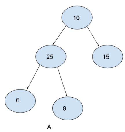
A. is a complete binary tree. Notice how every level except the last level is filled. Also notice how the last level is filled from left to right.
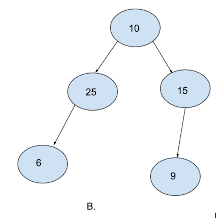
B. is not a complete binary tree. Although evey level is filled except for the last level. Notice how the last level is not filled from left to right. 25 does not have any right node and yet there is one more node (9) in the same level towards the right of it. It is mandatory for a complete binary tree to be filled from left to right.
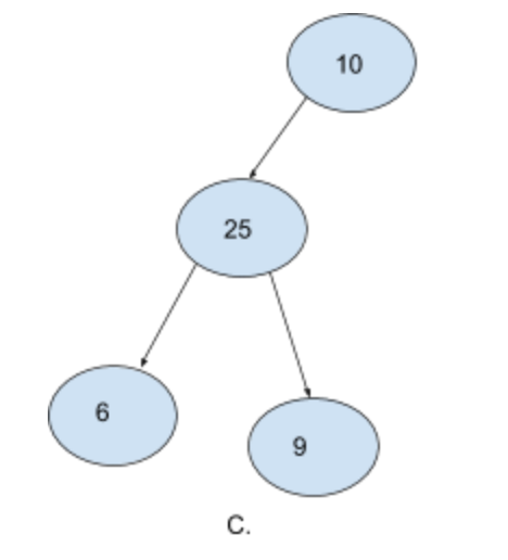
C. is also not a binary tree. Notice how the second level is not completely filled and yet we have elements in the third level. The right node of 10 is empty and yet we have nodes in the next level.
Heap Order Property - Heaps come in two flavors
* Min Heap
* Max Heap
- Min Heap - In the case of min heaps, for each node, the parent node must be smaller than both the child nodes. It’s okay even if one or both of the child nodes do not exists. However if they do exist, the value of the parent node must be smaller. Also note that it does not matter if the left node is greater than the right node or vice versa. The only important condition is that the root node must be smaller than both it’s child nodes
- Max Heap - For max heaps, this condition is exactly reversed. For each node, the value of the parent node must be larger than both the child nodes.
Heapify
Heap Implementation
Code: Heap Exercise
Hard
- Balanced Binary Tree
Max number of nodes in hth level= $2^{(h-1)}$
min number of nodes from 1st level to hth level =$2^{(h-1)}$max number of nodes from 1st level to hth level =$2^h - 1$
Thus, in a complete binary tree of height h, we can be assured that the number of elements n would be between these two numbers i.e.
$$ 2^{(h-1)} <= n <= 2^h - 1$$
- If we write the first inequality in base-2 logarithmic format we would have
$$ \log_{2}\ (2^{(h-1)}) <= \log_{2} n $$
$$or$$
$$ h <= \log_{2} n + 1$$
- Similarly, if we write the second equality in base-2 logarithmic format
$$ \log_{2} (n + 1) <= \log_{2}\ 2^{h}$$
$$ or $$
$$ \log_{2} (n + 1) <= h $$
Thus the value of our height h is always
$$ \log_{2} (n + 1) <= h <= \log_{2} n + 1$$
We can see that the height of our complete binary tree will always be in the order of O(h) or O(log(n))
So, if instead of using a binary search tree, we use a complete binary tree, both insert and remove operation
will have the time complexity $\ \log_{2} n$
We first inserted our element at the possible index.
Then we compared this element with the parent element and swapped them after finding that our child node was smaller than our parent node. And we did this process again. While writing code, we will continue this process until we find a parent which is smaller than the child node. Because we are travering the tree upwards while heapifying, this particular process is more accurately called
up-heapify.
Thus our insert method is actually done in two steps:
- insert
- up-heapify
Self-Balancing Tree
In addition to the requirements imposed on a binary search tree the following must be satisfied by a red–black tree:[18]
- Each node is either red or black.
- All NIL nodes (figure 1) are considered black.
- A red node does not have a red child.
- Every path from a given node to any of its descendant NIL nodes goes through the same number of black nodes.
Red-Black Tree Insertion
One overall rule of insertion rule is that you should try to insert a node as a red node.
Tree Rotations
Code: Build a Red-Black Tree
Unfinished
Sorting Algorithms
Introduction
Bubble Sort
Efficiency of Bubble Sort
Number of comparison: $(n-1)$
Number of steps: : $(n-1)$
Time Complexity: $(n-1)^2 = n^2 + 1 - 2n = n^2$
Space Complexity: $O(1)$
Code: Bubble Sort Exercise
Merge Sort
Divide and Conquer
Basic Algorithms
1 | class Solution: |
Efficiency of Merge Sort
Number of comparison: $n$
Number of steps: : $log(n)$
Time Complexity: $nlog(n)$
Space Complexity: $O(n)$
Code: Merge Sort Walkthrough
Code: Counting Inversions
Skip
Code: Case Specific Sorting of Strings
Skip
Quicksort

By en:User:RolandH, CC BY-SA 3.0, Link
Quicksort Efficiency
- Average: $O(nlog(n))$
- Worst case: $O(n^2)$
Code: Quicksort Walkthrough
Code: Heapsort
Unfinished
Based on Heap.
Code: Two Sum
Code: Sort 0, 1, 2
Unfinished
Faster Divide & Conquer Algorithms
Advanced Algorithms
Dynamic Programming
Knapsack Problem
Brute Force: 穷举法
Dynamic Programming: 动态规划
Exponential Time Algorithms: $O(2^n)$
Polynomial Time Algorithms: $O(n^2)$ or $O(3n)$
Smarter Approach
Dynamic Programming
Problem: Max value for weight limit
Subproblem: Max value for some smaller weight
Base Case: Smallest computation (Compute values for one object)
Lookup Table:
- 2, 6
- 5, 9
- 4, 5
| Weight | 0 | 1 | 2 | 3 | 4 | 5 | 6 |
|---|---|---|---|---|---|---|---|
| V (0, 0) | 0 | 0 | 0 | 0 | 0 | 0 | 0 |
| V (2, 6) | 0 | 0 | 6 | 6 | 6 | 6 | 6 |
| V (5, 9) | 0 | 0 | 6 | 6 | 6 | 9 | 9 |
| V (4, 5) | 0 | 0 | 6 | 6 | 6 | 9 | 11 |
Memoization: Storing precomputed values
Can I break this problem up into subproblems?